Reducing communication volume overhead in large-scale parallel SpGEMM

REDUCING COMMUNICATION VOLUME

OVERHEAD IN LARGE-SCALE PARALLEL

SPGEMM

a thesis submitted to

the graduate school of engineering and science

of bilkent university

in partial fulfillment of the requirements for

the degree of

master of science

in

computer engineering

By

Ba¸sak ¨

Unsal

December 2016

REDUCING COMMUNICATION VOLUME OVERHEAD IN LARGE-SCALE PARALLEL SPGEMM

By Ba¸sak ¨Unsal December 2016

We certify that we have read this thesis and that in our opinion it is fully adequate, in scope and in quality, as a thesis for the degree of Master of Science.

Cevdet Aykanat(Advisor)

M. Mustafa ¨Ozdal

Tayfun K¨u¸c¨ukyılmaz

Approved for the Graduate School of Engineering and Science:

Ezhan Kara¸san

ABSTRACT

REDUCING COMMUNICATION VOLUME

OVERHEAD IN LARGE-SCALE PARALLEL SPGEMM

Ba¸sak ¨Unsal

M.S. in Computer Engineering Advisor: Cevdet Aykanat

December 2016

Sparse matrix-matrix multiplication of the form of C = A× B, C = A × A and C = A× AT _{is a key operation in various domains and is characterized}

with high complexity and runtime overhead. There exist models for parallelizing this operation in distributed memory architectures such as outer-product (OP), inner-product (IP), row-by-row-product (RRP) and column-by-column-product (CCP). We focus on row-by-row-product due to its convincing performance, row preprocessing overhead and no symbolic multiplication requirement. The paral-lelization via row-by-row-product model can be achieved using bipartite graphs or hypergraphs. For an efficient parallelization, we can consider multiple volume-based metrics to be reduced such as total volume, maximum volume, etc. Existing approaches for RRP model do not encapsulate multiple volume-based metrics.

In this thesis, we propose a two-phase approach to reduce multiple volume-based cost metrics. In the first phase, total volume is reduced with a bipartite graph model. In the second phase, we reduce maximum volume while trying to keep the increase in total volume as small as possible. Our experiments show that the proposed approach is effective at reducing multiple volume-based metrics for different forms of SpGEMM operations.

Keywords: Parallel computing, combinatorial scientific computing, partitioning,

¨

OZET

B ¨

UY ¨

UK ¨

OLC

¸ EKL˙I PARALEL SYGEMM’DE ˙ILET˙IS

¸ ˙IM

HACM˙IN˙I D ¨

US

¸URME

Ba¸sak ¨Unsal

Bilgisayar M¨uhendisli˘gi, Y¨uksek Lisans Tez Danı¸smanı: Cevdet Aykanat

Aralık 2016

Seyrek matris-matris ¸carpımları (SyGEMM) bir ¸cok alanda en sık kullanılan operasyonlardan biridir. Bu i¸slemler genel olarak karma¸sık ve uzun ¸calı¸sma s¨urelerine ne sahiptir. Da˘gıtık bellek sistemlerinde bu i¸slemleri parallelle¸stirmek i¸cin bir ¸cok y¨ontem mevcuttur. Bunlar: dı¸s ¸carpım, i¸c ¸carpım, satır-satır ¸carpım ve s¨ut¨un-s¨ut¨un ¸carpımdır. Bu tezde, d¨u¸s¨uk ¨onhazırlık, iyi performans ve sembo-lik ¸carpma gerektirmemesi gibi bir ¸cok getirisinden dolayı satır-satır ¸carpımına yo˘gunla¸sılmı¸stır. Satır-satır ¸carpımının paralelle¸stirilmesinde iki-k¨umeli ¸cizgeler ve hiper ¸cizgeler kullanılabilmektedir.

Daha verimli bir paralle¸stirme i¸cin, toplam hacim ve en y¨uksek hacim gibi bir ¸cok hacim odaklı ¨ol¸c¨ut dikkate alınabilir. Satır-satır ¸carpımlar i¸cin var olan y¨ontemler, bir ¸cok hacim odaklı ¨ol¸c¨ut¨u aynı anda ger¸cekle¸stirmekte ba¸sarısız ol-maktadırlar.

Bu tezde, bir ¸cok hacim odaklı ¨ol¸c¨ut¨u aynı anda d¨u¸s¨urmek i¸cin iki a¸samalı bir y¨ontem ¨onerdik. ˙Ilk a¸samada, toplam hacim iki k¨umeli ¸cizge kullanılarak d¨u¸s¨ur¨ulm¨u¸st¨ur. ˙Ikinci a¸samada ise toplam hacimdeki artı¸sı en azda tutmaya ¸calı¸sarak en y¨uksek hacimi d¨u¸s¨urd¨uk.

Deneylerimizde g¨or¨ulebilmektedir ki, ¨onerdi˘gimiz y¨ontem ¸ce¸sitli SyGEMM i¸slemleri i¸cin bir ¸cok hacim odaklı ¨ol¸ce˘gi aynı anda d¨u¸s¨urm¨u¸st¨ur.

Anahtar s¨ozc¨ukler : Paralel i¸slemler, kombinasyonal bilimsel uygulamalar, seyrek

Acknowledgement

First and foremost, I owe my deepest gratitude to my supervisor, Prof. Dr. Cevdet Aykanat for his encouragement, motivation, guidance and support throughout my studies. Also, I would like to thank to Dr. O˘guz Selvitopi for an-swering my endless questions patiently and helping me whenever I face a problem about my studies.

Special thanks to Asst. Prof. Dr. Mustafa ¨Ozdal and Asst. Prof. Dr. Tayfun K¨u¸c¨ukyılmaz for kindly accepting to be in my committee. I owe them my appreciation for their support and helpful suggestions.

A very special thanks goes to my parents F¨usun and Yusuf for being there whenever I need them, to my sister Begum and my brother-in-law Alper for listening my endless complaints about everything and to my nephews Oreo and Toprak. This thesis have never been completed without their support.

Very valuable thanks to Ebru Ate¸s for everything she made for me. I would like to thank specially to Elif and Burak for cheering me up every time, to Seher for her wisdom and guiding me about every aspect of master. I am grateful to share enjoyable time with G¨ulfem and Kubilay before they left Ankara. I consider myself to be very lucky to have the most valuable friends from Bilkent, ˙Istemi, Simge, Necmi, Caner, Troya, Mehmet, G¨ulce, Shatlyk, Hamed, Noushin, ˙Ilker, Fahrettin, Sıtar, G¨und¨uz, Pelin and G¨ok¸ce. Also, I would like to thank to every single person I met in Bilkent for making Ankara liveable for me.

There are also motivations to make me return home. I am grateful to my friends from bachelor degree, Onurcan, Merve, C¸ isel, Aykut, C¨uneyt and to old friends, Ba¸sak, N¨uket, Alper, ˙Ilke, Alper D. and G¨oksu.

Lastly, I would like to thank to CS department for supporting me during my master study.

Contents

3.3 Parallelization of Sparse Matrix-Matrix Multiplication . . . 9

3.3.1 RRP and Representation of SpGEMM . . . 11

3.3.2 Partitioning of the Bipartite Graph . . . 15

3.3.3 Partitioning with fixed vertices . . . 17

CONTENTS vii

4.1 First Phase . . . 19 4.2 Second Phase . . . 19 4.2.1 A Bipartite Graph Model for Balancing Volume Loads . . 19 4.2.2 A Bin Packing Heuristic for Distributing Communication

Tasks . . . 23 4.2.3 Partitioning the Second Phase Bipartite Graph . . . 25

5 Experiments 28

5.1 Results for C = A× B . . . 30 5.2 Results for C = A× A . . . 33 5.3 Results for C = A× AT _{. . . . 41}

List of Figures

3.1 Example data dependencies between rows of A and B. . . . 13

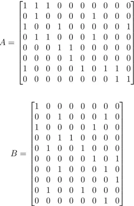
3.2 Examples of A (8× 10) and B (10 × 8) matrices. . . 13

3.3 Representation of matrices A and B via a bipartite graph. . . . . 14

3.4 A and B matrices after partitioning. . . . 15

3.5 Bipartite model after partitioning . . . 16

4.1 Representation of boundary vertices and cut edges. . . 21

4.2 Second phase bipartite graph. . . 22

4.3 Illustration of the bin packing algorithm. . . 24

4.4 Result of the bin packing algorithm. . . 25

4.5 Graph after second phase graph partitioning. . . 26

5.1 Comparison of maximum volume values for C = A× B . . . 33

5.2 Comparison of maximum volume values for C = A× A . . . 41

List of Tables

4.1 Status of the vertices after each phase. . . 27

5.1 Properties of input matrices. . . 29

5.2 Instances of C = A× B . . . 30 5.3 C = A× B, K = 256 . . . 31 5.4 C = A× B, K = 512 . . . 31 5.5 C = A× B, K = 1024 . . . 32 5.6 C = A× A, K = 256 . . . 35 5.7 C = A× A, K = 512 . . . 38 5.8 C = A× A, K = 1024 . . . 40 5.9 C = A× AT_{, K = 256 . . . . 43} 5.10 C = A× AT, K = 512 . . . . 44 5.11 C = A× AT_{, K = 1024 . . . . 45}

Chapter 1

Introduction

Sparse matrix-matrix multiplication (SpGEMM) in the form of C = A × B,

C = A× A and C = A × AT _{is a kernel operation for many scientific}

applica-tions. It may arise in linear programming [1], molecular dynamics [2] [3], breadth-first search [4], triangle counting in graphs [5] and recommendation systems [6]. Data used in those applications generally contain large sparse matrices and often computations on those matrices constitute computational bottlenecks. Hence, SpGEMM operations are parallelized to avoid long computation time. There exit different partitioning schemes for parallel SpGEMM; outer-product (OP), inner-product (IP), row-by-row-product (RRP) and column-by-column-product (CCP). Among these, RRP exhibits better parallelization performance due to the lower preprocessing overhead and requiring no symbolic multiplications. Those properties and advantages make RRP attractive compared to other models for parallelizing SpGEMM on distributed architectures.

In row-by-row-product parallelization, rows of A and rows of B are partitioned into K parts. After partitioning, an atomic task corresponds to multiplication of each nonzero in a row of A with the corresponding rows of B. This multiplication refers to computation task of the processor Pk that holds respective row of A. To

perform the computational tasks, the needed data should be transferred between processors, which necessitate communication tasks. Thus, partitioning into K

parts requires distributing communication and computational tasks among K processors. Distributing communication tasks leads to an optimization problem related to minimizing amount of volume of data sent over processors, including

total communication volume and maximum communication volume.

For RRP models, in the literature, there exist graph and hypergraph models in which rows represent vertices and nonzeros represent edges or hyperedges. These models aim to minimize volume-based metrics. Graphs used for RRP model are bipartite graphs. The existing bipartite graph model [7] fails to minimize multiple volume metrics at the same time and it fails to provide balanced communication tasks if the number of nonzeros in the rows has high variance,

This thesis introduces a two-phase bipartite graph model to reduce total and maximum volume sent over processors. In the first phase, total volume is mini-mized using bipartite graph model. In the second phase, the proposed bipartite model decreases the maximum communication volume while trying to keep the increase in total volume as small as possible. In other words, second phase tries to balance the communication loads of the processors. The proposed model in the second phase is orthogonal to the partitioning model used in the first phase. In other words, it can work with any readily partitioned instance.

Our comprehensive experiments demonstrate that our model balances maxi-mum communication volume as expected while keeping total volume found in the first phase almost the same.

Chapter 2

Related Work

There exist plenty of applications about optimizing matrix or matrix-vector multiplication problem for shared memory [8] [9] and distributed memory [10] [11] [12] [7] [13] architectures. Matrices used in those kernels can be large, containing million number of rows or columns. There are plenty of important volume-based cost metrics to consider for an efficient parallelization such as max-imum volume sent by a processor, total volume, volume imbalance, total message and maximum message sent or received. The approaches in the literature can be categorized into two as one-phase or two-phase according to way they address multiple communication cost metrics.

2.1

One-phase approaches

Recently, Deveci et al. [10] extended their early proposed algorithm called UMPa, which only decrease maximum communication volume, to a multilevel hypergraph partitioning tool that can handle multiple cost metrics such as total volume, max-imum communication volume, total and maxmax-imum number of messages simulta-neously. In this method, directed hypergraphs are used for modelling number of messages received and sent from processors and maximum volume. In other

words, UMPa is compared with tools such as PaToH, Mondriaan and Zoltan. Comparisons are done with 128, 256, 512 and 1024 processors and a large num-ber of example data sets show that UMPa obtains better results in terms of multiple communication cost metrics. For example, comparisons with PaToH in-dicate that, for 1024 processors, UMPa obtains 20% lower maximum number of messages sent by a processor and 14% lower total number of messages.

Acer et al. [11] focused on a model for sparse matrix dense matrix multipli-cation (SpMM) on distributed memory systems to decrease the cost of different volume metrics. Applications that belong to linear algebra operations and big data analysis utilizing SpMM causes high communication volume. The model presented in this work uses two different structures: graphs and hypergraphs. Using recursive bipartitioning in a single partitioning phase, their model tries to optimize not only total volume but also maximum send and receive volume. Experiments show that their graph model is 14.5 times faster than UMPa that ad-dresses similar communication metrics. Besides running time, their graph model also increases the quality of the partitions by 3% in terms of maximum volume. Their hypergraph model has a higher improvement rate of 13% on partition qual-ity and is also 3.4 times faster tham UMPa.

Recently, Slota et al. [14] presented a new partitioning tool called PuLP (Par-titioning using Label Propagation) tailored for scale-free graph that arise in big data. Parallelization is crucial in this area since input data is generally too com-plex and consume considerable energy and execution time when it is applied in distributed systems. Since label propagation algorithm, which is an example of agglomerative clustering, takes less time and can be easily parallelized producing results with acceptable quality. Besides satisfying partitioning constraints, PuLP also tries to minimize multiple edge and volume costs at the same time. Accord-ing to the experiments, PuLP outperforms METIS (which uses k-way multilevel partitioning algorithm) in terms of total edge cut and maximal cut edges per partition. Statistics shown in the paper indicate that PuLP consumes 8-39 times less memory compared to its alternatives. It is also mentioned that, the execution time of PuLP can be shorter than the state-of-art methods 14.5 times on average.

Although some of the approaches in the literature achieve quite successful partitioning results, there are some drawbacks using a single-phase approach. First of all, those methods may need to sacrifice some of the metrics to optimize others because it is difficult if not impossible to optimize multiple metrics at the same time in a single phase.

2.2

Two-phase approaches

Akbudak et al. [7] proposed a hypergraph and a bipartite graph model for par-allelization of outer-product, inner-product and row-by-row-product SpGEMM. This method consists of two phases to minimize multiple communication cost metrics. In the first phase, their approach creates a hypergraph or graph that is also called computational models. Aim of this step is to reduce the total message volume and balance the computational loads of the processors. Following this step, the second phase constructs another hypergraph representing communica-tion tasks to minimize the total message count and balance message volume loads of the processors. According to the experiments in the paper, for the first phase, bipartite graph is preferred to its hypergraph counterpart because of its low par-titioning overhead and construction cost although its efficiency is insignificantly low. Also in the experiments, they show that by decreasing latency and the band-width costs using communication hypergraph, time required for SpGEMM can be decreased up to 32%.

Similarly, Bisseling et al. [12] worked on finding proper partitioning for par-allel matrix-vector multiplication. In their model, they assume that the sparse matrix has already been partitioned and given as an input to the proposed ap-proach. They apply their algorithms to find suitable partitions for input and output vectors. A new lower bound is defined for maximum communication load of processors. One of their algorithm, called Opt2, can find the optimal solution which reach that predefined lower bound in a particular occurrence of the matrix such that each column of the matrix can be partitioned into at most two proces-sors in input vector. Additionally, there exists another heuristic called LB that

is successful in finding good solutions in practice providing that it is followed by a greedy algorithm.

In [13], Ucar et al. presented a solution to overcome the problem of partitioning of unsymmetric square and rectangular sparse matrices thar are used in matrix-vector multiplications. Although major part of the current partitioning models try to minimize total message volume, total message latency is also important metric to be considered. That is because sometimes start-up time required by a message can be longer than sending another message in the same package. To that end, they propose a two-phase methodology to minimize multiple communi-cation costs. In the first phase, besides computational load balance, objective is to reduce message volume using existing 1D partitioning models. The following phase takes the result of the first phase as an input and creates a communication hypergraph using relations between vertices and processors. This phase aims to minimize total message volume and balance work load of processors using hyper-graph partitioning. Results obtained from multiplication of parallel matrix-vector and matrix-transpose-vector using Message Passing Interface (MPI) indicate that, their model obtains considerable improvements over existing approaches.

It can be inferred that two-phase methods are more successful on optimizing multiple communication metrics. However, for both one- and two-phase methods, existing models fall short in the existence of communication tasks with non-uniform sizes.

Chapter 3

Background

3.1

Graph Partitioning

Standard graph model is represented as G = (V, E) where V represents the vertex set and E represents the edge set. Vertex vi in the vertex set may be connected

to other vertex vj via edge eij. In this case, vj is called neighbor of vi. Adj(vi)

contains the set of neighbors of vi which can be denoted as

Adj(vi) ={vj : eij ∈ E}.

Both edge eij and vertex vi may be associated with a cost cij and wi respectively.

Π(G) = {V1, ...,VK} shows a K-way partition of the graph G where K is the

number of processors or partitions. Π(G) consists of K set of vertices where Vk

represents the vertex set which are assigned to part k. In the partition Π(G) there can be two different types of edges, cut and uncut. If there exists an edge

eij between vi and vj that are assigned to different partitions, eij is called as a cut

edge. If the vertices vi and vj are in the same partition, eij is said to be uncut.

The total cutsize is given as

∑

eij∈EE

cij,

vi have a cut edge, in other words, if the vertex have a connection with a vertex

vj that is in another partition, both vertex vi and vj are called boundary

ver-tices. Boundary vertices necessitate communication in the system which will be specified as communication volume later in this section.

Sum of the weights of each vertex inVk denotes the weight of the partitionVk

which is denoted as W (Vk). There exists a balance criteria for a partition,

W (Vk)≤ Wavg(1 + ε), k∈ {1, ..., K}

where ε is imbalance value defined beforehand and Wavg is the average of the

weights of the partitions, i.e., ∑_kWc

avg(Vk)/K.

3.2

Sparse Matrices

For the representation of the graph, matrices are commonly used because of ease of computation and construction. According to the structure of the data to be stored, matrix may be sparse or dense.

• Sparse matrix: Most of the data is zero.

• Dense matrix: Number of nonzeros is greater than the number of zero ones.

Since in sparse matrices, most of the data is zero, storing it in a two-dimensional array structure is costly. Thus, there are couple of data structures to represent sparse matrices efficiently. The three common ones are,

1. Coordinate format (COO) : All entries are stored in a list which is in (row,

column, value) format.

2. Compressed sparse row (CSR) : In this commonly preferred representation technique, matrix is represented using three different lists:

(a) IA: starts with 0 and stores the cumulative number of nonzeros in each row. List has (#of rows) + 1 elements and ends with the total number of nonzero in the matrix.

(b) JA: stores the column value of each nonzero starting from the first row. This array consist of total number of nonzeros.

(c) A: consist of the nonzero values of the entries starting from top-left which is also have the same order as JA.

In case vertices or edges have weights, they can be stored in two different additional lists.

It provides fast data access without searching for data as in COO. Example 3.1 shows how to construct CSR for an example matrix M.

M =       0 2 0 0 1 0 0 4 0 0 0 0 0 0 3 0       IA = [0 1 3 3 4] J A = [1 0 3 2] A = [2 1 4 3] (3.1)

3. Compressed sparse column (CSC) : This representation is quite similar to CSR. The only difference is that, columns are taken into account in IA instead of rows. In other words, CSC works like reverse of CSR.

3.3

Parallelization

of

Sparse

Matrix-Matrix

Multiplication

In scientific applications, one of the most common and crucial operations is sparse matrix-matrix multiplication (SpGEMM). Since the matrices used in those ap-plications may have large number of rows and columns and high complexity,

sequential execution leads long running time. Therefore, parallelization of the multiplication becomes imperative. In the literature, there are four common ways to parallelize SpGEEM: outer-product-parallel, inner-product-parallel, row-by-row-product-parallel, column-by-column-product-parallel.

Taking C = A× B into account, these parallelization schemes work as follows: 1. Outer-product-parallel algorithm (OP): Columns of A and rows of B are mapped to the processors. In the computation, the elements in the column of A and the corresponding row of B are accessed once by the processors. After this operation, partial results are produced which means outer prod-ucts may contribute to the same element in the output matrix C. Thus, elements of the C are needed to be accessed more than once.

2. Inner-product-parallel algorithm (IP): Rows of A and columns of B are mapped to the processors. In the computation, each multiplication calcu-lates the result of only one element in C. Therefore, the elements of the C are accessed once by the responsible processor.

3. Row-by-row-product-parallel algorithm (RRP): Both A and B are parti-tioned rowwise. Elements in the rows of B are multiplied by the rows of

A. Therefore, while nonzeros in the rows of A are used for computing once,

rows of B are accessed more than once.

4. Column-by-column-product-parallel algorithm (CCP): Both A and B are partitioned columnwise. This algorithm works like reverse of the RRP. In other words, columns of B are used for computing once, whereas, the columns of A are accessed more than one. In both RRP and CCP, the elements of output matrix of the C are accessed once by the responsible processors.

As mentioned in previous sections, using RRP in parallelization of SPGEMM is more effective than using OP and IP in terms of speed and partitioning per-formance. Therefore, in this thesis, we focus on improving performance of RRP model.

3.3.1

RRP and Representation of SpGEMM

In RRP model, rows of A (ai∗) and B (bj∗) are mapped to the processors. The

main operation is the multiplication of each nonzero aij in ai∗ with all nonzero

elements in bj∗. The atomic task regarding ith row of A is defined as

{ai,jbj,∗ : j ∈ cols(ai,∗)}.

Data used in the atomic multiplication can be assigned to different processors. Therefore, it may be needed to be sent over partitions. Transferring data in-curs communication in the system. We can categorize the operations in RRP SpGEMM as computational and communication tasks. Since every row of B is multiplied by each nonzero in the corresponding row of A, the computational tasks are defined on rows of A. Whereas, due to the fact that nonzeros in the rows of B are needed to be sent for the computational tasks, the communication tasks are defined on rows of B.

Bipartite graphs are specialized graphs that consist of disjoint sets of vertices. They constitute a natural way to model sparse matrix-matrix multiplication. Bipartite graph model only allows edges or connections between disjoint sets of vertices. We use following notation to represent RRP SpGEMM as a bipartite graph.

GRRP ={VrrAC∪ VrB,EzA}

In the existing bipartite graph model [7], number of rows of A and number of row of B together give the number of vertices inGRRP. Each row of A is represented

as a vertex in VAC

rr and each row of B is represented as a vertex in VrB set. The

number of edges in the graph is equal to the number of nonzeros in matrix A because each nonzero in A signifies a dependency to a row B, that is captured with an edge. An edge eij in edge set EzA connects a vertex vi with a vertex vj.

{EA

z = eij : vi ∈ VrrAC, vj ∈ VrB}

Adjacency list of vi denotes the set of vertices are neighbor of vi. In SpGEMM, it

represents the rows of B that should be received by vi to perform multiplication.

Similarly, adjacency list of vj consist of the neighbors of vj. In other words,

Adjacency list of vj includes the computational tasks which need the respective

row of B for their computation.

Adj(vj) = {vi : i∈ rows(a∗,j)}

In the bipartite graph model, there are also weights for both edges and vertices. Weight of vertex viis calculated as computational load of the multiplication which

can be also identified as the sum of number of nonzeros in each row of B that is needed for multiplication with the respective row of A:

w(vi) =

∑

j∈cols(ai,∗)

#nonzero(bj,∗).

The vertices that belong to B do not have any weights because, they do not represent any computation tasks.

In the graph model, there also exist edge weights. Each vertex vj determines

the cost of its edges. For instance, for vertices vi and vj, the cost of eij is assigned

as the number of nonzeros in vj. This is given by

c((vi, vj)) = c(eij) = cij = #nonzero(bj,∗).

Expression of the formulations is shown on the example graph in Figure 3.1. In Figure 3.1, ai1,∗, . . . , ai4,∗ denote the computational tasks and arrows indicate the

data dependencies. For instance, in the graph, vertex ai1,∗ needs three different

rows bj1,∗, bj2,∗ and bj3,∗. Therefore, the processors that store these rows of B

should send them to the processor that stores ai1,∗ prior to multiplication.

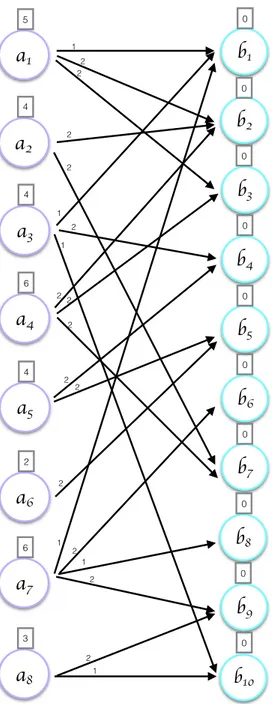
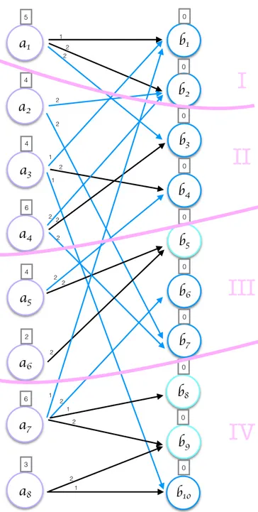
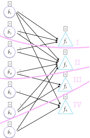
Figure 3.2 is given as an example for matrices A and B and Figure 3.3 il-lustrates the bipartite graph model that represents the SpGEMM operation

C = A× B. In the Figure 3.3, purple vertices represent rows of A whereas,

green ones represent rows of B. Numbers on the edges stand for the weights of them. Similarly rectangular areas above the vertices indicate their weights.

a

a

a

a

b

b

b

a

a

a

a

a

a

a

Figure 3.1: Example data dependencies between rows of A and B.

A =             1 1 1 0 0 0 0 0 0 0 0 1 0 0 0 0 1 0 0 0 1 0 0 1 0 0 0 0 0 1 0 1 1 0 0 0 1 0 0 0 0 0 0 1 1 0 0 0 0 0 0 0 0 0 1 0 0 0 0 0 1 0 0 0 0 1 0 1 1 0 0 0 0 0 0 0 0 0 1 1             B =                 1 0 0 0 0 0 0 0 0 0 1 0 0 0 1 0 1 0 0 0 0 1 0 0 0 0 1 1 0 0 0 0 0 1 0 0 1 0 0 0 0 0 0 0 0 1 0 1 0 0 1 0 0 0 1 0 0 0 0 0 0 0 0 1 0 1 0 0 1 0 0 0 0 0 0 0 0 0 1 0                

a

a

a

a

a

a

a

a

b

b

b

b

b

b

b

b

b

I

II

III

For the model, there also exist edge weights. Every vertex vj determines the

edge cost of its edges. For instance, for vertices viand vj, cost of the eijis assigned

as number of nonzero in vj. It can also be defined as

c((vi, vj)) = c(eij) = cij = #nonzero(bj,⇤)

Expression of the formulations is shown on the example graph in 3.1. In the figure, rows of A and B markes as purple. Arrows represents shared nonzero between A and B.

An example matrix (3.2) and a graph (3.3) can be seen below. In the figure, purple vertices represents rows of A whereas, green ones are rows of B. Numbers on the edges shows the weights of them. Similarly rectangular areas on the vertices indicates weights.

A = 2 6 6 6 6 6 6 6 6 6 6 4 1 1 1 0 0 0 0 0 0 0 0 1 0 0 0 0 1 0 0 0 1 0 0 1 0 0 0 0 0 1 0 1 1 0 0 0 1 0 0 0 0 0 0 1 1 0 0 0 0 0 0 0 0 0 1 0 0 0 0 0 1 0 0 0 0 1 0 1 1 0 0 0 0 0 0 0 0 0 1 1 3 7 7 7 7 7 7 7 7 7 7 5 , B = 2 6 6 6 6 6 6 6 6 6 6 6 6 6 6 4 1 0 0 0 0 0 0 0 0 0 1 0 0 0 1 0 1 0 0 0 0 1 0 0 0 0 1 1 0 0 0 0 0 1 0 0 1 0 0 0 0 0 0 0 0 1 0 1 0 0 1 0 0 0 1 0 0 0 0 0 0 0 0 1 0 1 0 0 1 0 0 0 0 0 0 0 0 0 1 0 3 7 7 7 7 7 7 7 7 7 7 7 7 7 7 5

Figure 3.2: Examples of A and B matrices

10 For the model, there also exist edge weights. Every vertex vj determines the

edge cost of its edges. For instance, for vertices viand vj, cost of the eij is assigned

as number of nonzero in vj. It can also be defined as

c((vi, vj)) = c(eij) = cij = #nonzero(bj,⇤)

Expression of the formulations is shown on the example graph in 3.1. In the figure, rows of A and B markes as purple. Arrows represents shared nonzero between A and B.

An example matrix (3.2) and a graph (3.3) can be seen below. In the figure, purple vertices represents rows of A whereas, green ones are rows of B. Numbers on the edges shows the weights of them. Similarly rectangular areas on the vertices indicates weights.

A = 2 6 6 6 6 6 6 6 6 6 6 4 1 1 1 0 0 0 0 0 0 0 0 1 0 0 0 0 1 0 0 0 1 0 0 1 0 0 0 0 0 1 0 1 1 0 0 0 1 0 0 0 0 0 0 1 1 0 0 0 0 0 0 0 0 0 1 0 0 0 0 0 1 0 0 0 0 1 0 1 1 0 0 0 0 0 0 0 0 0 1 1 3 7 7 7 7 7 7 7 7 7 7 5 , B = 2 6 6 6 6 6 6 6 6 6 6 6 6 6 6 4 1 0 0 0 0 0 0 0 0 0 1 0 0 0 1 0 1 0 0 0 0 1 0 0 0 0 1 1 0 0 0 0 0 1 0 0 1 0 0 0 0 0 0 0 0 1 0 1 0 0 1 0 0 0 1 0 0 0 0 0 0 0 0 1 0 1 0 0 1 0 0 0 0 0 0 0 0 0 1 0 3 7 7 7 7 7 7 7 7 7 7 7 7 7 7 5

Figure 3.2: Examples of A and B matrices

10

IV

I

II

III

IV

I

II

III

For the model, there also exist edge weights. Every vertex v

determines the

edge cost of its edges. For instance, for vertices v

and v

, cost of the e

is assigned

as number of nonzero in v

. It can also be defined as

c((v

, v

)) = c(e

) = c

= #nonzero(b

)

Expression of the formulations is shown on the example graph in 3.1. In the

figure, rows of A and B markes as purple. Arrows represents shared nonzero

between A and B.

An example matrix (3.2) and a graph (3.3) can be seen below. In the figure,

purple vertices represents rows of A whereas, green ones are rows of B. Numbers

on the edges shows the weights of them. Similarly rectangular areas on the

vertices indicates weights.

A =

2

6

6

6

6

6

6

6

6

6

6

4

1 1 1 0 0 0 0 0 0 0

0 1 0 0 0 0 1 0 0 0

1 0 0 1 0 0 0 0 0 1

0 1 1 0 0 0 1 0 0 0

0 0 0 1 1 0 0 0 0 0

0 0 0 0 1 0 0 0 0 0

1 0 0 0 0 1 0 1 1 0

0 0 0 0 0 0 0 0 1 1

3

7

7

7

7

7

7

7

7

7

7

5

, B =

2

6

6

6

6

6

6

6

6

6

6

6

6

6

6

4

1 0 0 0 0 0 0 0

0 0 1 0 0 0 1 0

1 0 0 0 0 1 0 0

0 0 1 1 0 0 0 0

0 1 0 0 1 0 0 0

0 0 0 0 0 1 0 1

0 0 1 0 0 0 1 0

0 0 0 0 0 0 0 1

0 1 0 0 1 0 0 0

0 0 0 0 0 0 1 0

3

7

7

7

7

7

7

7

7

7

7

7

7

7

7

5

Figure 3.2: Examples of A and B matrices

10

For the model, there also exist edge weights. Every vertex v

determines the

edge cost of its edges. For instance, for vertices v

and v

, cost of the e

is assigned

as number of nonzero in v

. It can also be defined as

c((v

, v

)) = c(e

) = c

= #nonzero(b

)

Expression of the formulations is shown on the example graph in 3.1. In the

figure, rows of A and B markes as purple. Arrows represents shared nonzero

between A and B.

An example matrix (3.2) and a graph (3.3) can be seen below. In the figure,

purple vertices represents rows of A whereas, green ones are rows of B. Numbers

on the edges shows the weights of them. Similarly rectangular areas on the

vertices indicates weights.

A =

2

6

6

6

6

6

6

6

6

6

6

4

1 1 1 0 0 0 0 0 0 0

0 1 0 0 0 0 1 0 0 0

1 0 0 1 0 0 0 0 0 1

0 1 1 0 0 0 1 0 0 0

0 0 0 1 1 0 0 0 0 0

0 0 0 0 1 0 0 0 0 0

1 0 0 0 0 1 0 1 1 0

0 0 0 0 0 0 0 0 1 1

3

7

7

7

7

7

7

7

7

7

7

5

, B =

2

6

6

6

6

6

6

6

6

6

6

6

6

6

6

4

1 0 0 0 0 0 0 0

0 0 1 0 0 0 1 0

1 0 0 0 0 1 0 0

0 0 1 1 0 0 0 0

0 1 0 0 1 0 0 0

0 0 0 0 0 1 0 1

0 0 1 0 0 0 1 0

0 0 0 0 0 0 0 1

0 1 0 0 1 0 0 0

0 0 0 0 0 0 1 0

3

7

7

7

7

7

7

7

7

7

7

7

7

7

7

5

Figure 3.2: Examples of A and B matrices

10

IV

I

II

III

IV

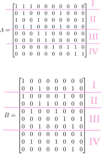
Figure 3.4: A and B matrices after partitioning.

3.3.2

Partitioning of the Bipartite Graph

In the literature, there exist several tools for obtaining 1D partitioning on ma-trices. Metis [15], Scotch [16] and PuLP [14] are the tools among common ones. Using any of these partitioners, we can obtain a K-way partition as Π ={V1, . . . ,VK}.

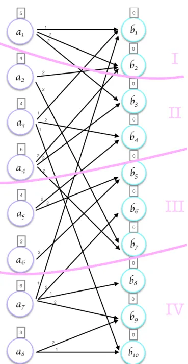
As can be seen in Figures 3.4 and 3.5, bipartite graph is partitioned into K = 4 parts. In the figure, partition 1 has a1 and b1, b2, partition 2 has a2, a3, a4, b3, b4,

partition 3 has a5, a6, b5, b6, b7, partition 4 has a7, a8, b8, b9, b10. In this graph,

computation and communication costs can be also inferred. Recall that a vertex having an edge to a vertex in a different partition was called boundary vertex

a

a

a

a

a

a

a

a

b

b

b

b

b

b

b

b

b

I

II

III

IV

such as a1, a2, a3, a5 and a7. Boundary vertices incur communication overhead

as much as their weights.

Since a1 requires b1, b2 and b3 to compute first row of C, processor 2 and

pro-cessor 3 needs to send b2 and b3 respectively. Because the number of nonzeros

defines weight of the vertices, which is also the amount of computation, compu-tational load of a processor can be found as the sum of the weights of vertices in that processor. For vertices of B, this weight is 0 because they do not signify any computation. In this case of example graph, computational load of processor 3 is 4 + 2 + 0 + 0 + 0 = 4.

3.3.3

Partitioning with fixed vertices

In the problem of partitioning and repartitioning, fix vertices are commonly used. Difference of this partitioning from the regular one is that there is constraint for the part assignment of specific vertices. In this type of assignment, those specific vertices, which are also called fixed vertices, have predefined partition values that are specified before part assignment operation. For the set of the fixed vertices which belongs to part VK is shown asFK for k = 1, . . . , K. Regular partitioning

step is applied to remaining free vertices which are denoted as V − {F1∪ F2∪

Chapter 4

Proposed Method

In the scientific applications, the input matrices in SpGEMM may be related ac-cording to the applications’ specific needs In other words, SpGEMM can represent three different types of operations:

• C = A × B : represents the multiplication of two different sparse matrices • C = A × A : represents the multiplication of matrix with itself

• C = A × AT _{: represents the multiplication of matrix with its transpose}

where A and B are sparse matrices. Regardless of the type of the operation and form of the matrices, bipartite graphs are used for modelling purpose. Different types of the operation do not require any alteration in the model.

In this thesis, we propose a new two-phase approach to reduce maximum volume and total volume. This two-phase approach also satisfies balanced com-putational work load on processors for RRP SPGEMM. In the first phase, the aim is to minimize the total communication volume. In the second phase, the aim is to reduce the maximum volume while keeping the increase in total volume found in the first phase as small as possible.

4.1

First Phase

First phase consist of existing state-of-art RRP SPGEMM partitioning method as described in previous sections. C = A× B is represented with a bipartite graph, where rows of A and B are represented by the vertices and nonzeros needed for rows of A constitute the edges. This graph shows computational dependencies among row vertices. The aim of first phase is to reduce total volume of processors. At the end of this phase, we obtain K-way partition Π1 for both rows of A and

B, denoted as

Π1 ={V1,V2, ...,VK}

In the first phase, we choose Metis to partition the graph due to its success in reducing volume and balancing computational loads.

4.2

Second Phase

After reducing total volume in the first phase, the aim of the second phase is to reduce maximum communication volume sent by a processor and hence balance the communication loads of processors. This phase takes the result of the first phase as an input and applies two different methods for satisfying objectives mentioned above.

4.2.1

A Bipartite Graph Model for Balancing Volume

Loads

Generating the second phase bipartite graph follows similar steps with the one in the first phase. Since the graph in this phase represents the communication tasks, the aim of this phase is to reduce maximum communication volume of the processors, we call this graph a communication graph (Vcomm). In the graph

1. Boundary vertices (VB′): In the bipartite graph of the first phase, a vertex

bi in VrB which has an outer edge is added to the set VB′. That is because

only the vertices inVB

r participate in communication tasks.

VB′ ={bi : bi ∈ VB and bi is boundary}

2. Fixed vertices (VF): Vertices in VF represent processors. Therefore, the

number of fixed vertices is equal to the number of processors. These vertices do not have weights. Each fixed vertex fj has a predefined partition, which

is one of the processors.

VF ={fj : fj is a fixed vertex and 1≤ fj ≤ K}

Thus, the new vertex set can be denoted as:

Vcomm ={VB′ ∪ VF}.

Each edge eij connects a vertex bi in VB′ and a fixed vertex fj in VF. The

edge is formed if there is a connection between a vertex and a processor. In other words, every boundary vertex has an edge between partition of its neighbors since it incurs communication. It can be denoted as:

Ecomm ={eij : vi ∈ VB′, vj ∈ VF, Adj(vi)∩ Vj ̸= ∅}.

When all those formulations are combined in a graph, we have

a

a

a

a

a

a

a

a

b

b

b

b

b

b

b

b

b

I

II

III

IV

b

b

b

b

b

b

b

f

f

f

f

Figure 4.2: Second phase bipartite graph.

In the Figure 4.1, the boundary vertices such as b1, b2, b3, b4, b6, b7, b10 are

marked as blue with the cut edges. For instance, for vertex b1, there are three

incoming edges: one is from partition 2, other is from partition 4 and the last one is an internal edge. In this case, edges from a3 and a7 cause communication

that are both from the same partition as b5. Thus, it is not added to the new

bipartite graph because there is no necessity for communicating b5.

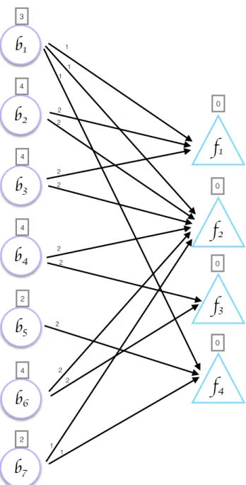
Figure 4.2 shows the second phase bipartite graph model as an example. Circle vertices represent the boundary vertices, triangle ones represent the fixed ones. All relations are inferred from Figure 4.1. Edge weights are defined as the weights of boundary vertices:

cij = c(eij) = #nonzero(vi).

Since fixed vertices do not incur communication, their weights are zero. Weights of the vertices in VB′ are calculated as the sum of weights of outgoing edges.

4.2.2

A Bin Packing Heuristic for Distributing

Commu-nication Tasks

As a baseline method, we use a variant of bin packing algorithm. In this heuristic, each processor is represented with a bin and each vertex is seen as an item to be assigned to the bins.

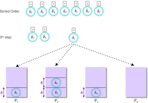
Algorithm 1 displays the bin packing algorithm. This algorithm takes the

Gcomm as an input. In the first step, all vertices except the fixed ones are sorted

in descending order in terms of their weights. Starting from the vertex with the highest weight, they are assigned to the bins (processors) with the current lowest weight, which is one of the neighbors of that vertex (an illustration is given in Figure 4.3 and 4.4). The reason behind this is not to increase the load of the processor with the highest volume. This method also guarantees that no vertex is assigned to the part that is not in its neighbor list. For example, In Figure 4.1, vertex a2 is assigned to partition 2, however, all of its neighbors are in different

partitions (Partition 1 and 3). Since we are picking the processor to be assigned in adjacency list of the vertex, for this phase, this bin packing heuristic avoids from such cases.

Data: Second phase bipartite graph Gcomm

Result: Partition vector of graph Gcomm

Sort vertices according to their weights in descending order; while there exist an unassigned vertex vi do

Find Adj(vi);

Sort Adj(vi) in ascending order;

Assign vi to the processor pk ∈ Adj(vi) with the lowest total weight;

Update pk;

end

Algorithm 1: Bin packing algorithm.

P1 P2 P3 P4 b7 2 b5 2 b1 3 b3 b2 b4 b6 Sorted Order: b₂ 4 b3 4 b4 b6 4 b1 b5 2 b7 2 3 4 5th _step: 4 4 4 4

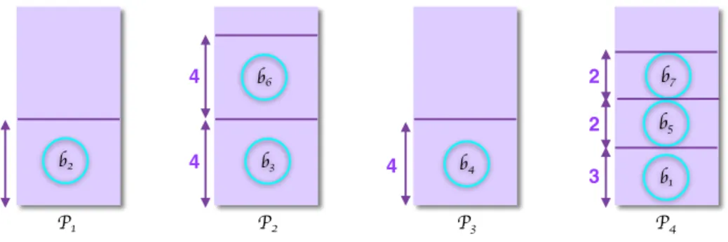
P1 P2 P3 P4 b7 b5 b1 b3 b2 b4 b6 4 4 4 4 ₃ 2 2

Figure 4.4: Result of the bin packing algorithm.

4.2.3

Partitioning the Second Phase Bipartite Graph

For reducing maximum volume, we apply partitioning to the second phase bipar-tite graph.

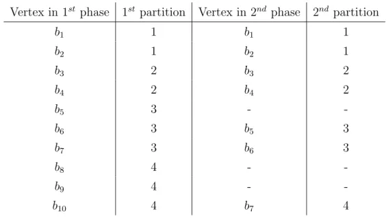
Although bin packing heuristic guarantees to avoid assigning a vertex to the part which is not in the adjacency list of it, it may still cause some misassignments. For example, a vertex may have multiple neighbors in partition i, but, if there is another empty bin, it may be assigned to it. In this case, satisfying objectives may be failed. Using graph partitioning may provide more successful results in such cases. In Figure 4.5 and in Table 4.1, status of the vertices and graph after partitioning can be seen.

In this phase, it can be seen that only the placement of rows of B are changed. Since total volume calculated in the first phase does depend on the rows of A, after this phase, it is unlikely to increase since the partitioner will avoid making out-of-part assignments in order to not to increase cutsize. The assigned vertices are the boundary vertices of B and the partitioner is unlikely to assign vertices to the processors to the processors that is not in its neighbor list. By this means, total volume can be kept small and volume loads of the processors can be balanced by maintaining a balance on the part weights in the graph. Recall that the total messages of the vertices in a part corresponds to the send volume of the respective

processor. By feeding the law, imbalance threshold to the underlying partitioner, we can control the maximum volume and reduce it.

b1 3 b2 4 b3 4 b4 4 b5 2 b6 4 b7 2 f1 f2 f3 f4 1 1 1 2 2 2 2 2 2 2 2 2 1 1 0 0 0 0

I

II

III

IV

Vertex in 1st phase 1st partition Vertex in 2nd phase 2nd partition b1 1 b1 1 b2 1 b2 1 b3 2 b3 2 b4 2 b4 2 b5 3 - -b6 3 b5 3 b7 3 b6 3 b8 4 - -b9 4 - -b10 4 b7 4

Chapter 5

Experiments

Both bin packing and graph partitioning methods are tested on three forms of SpGEMM

C = A× B,

C = A× A,

C = A× AT.

Approaches mentioned in Section 4 are applied on a large set of matrices retrieved from matrix market of University of Florida [17]. Those matrices are from real applications and also they are sparse. Names of the matrices used for each operation can be seen below.

• C = A × B : amazon0302, amazon0312, thermomech dK

• C = A × A : 2cubes sphere, 598a, bfly, cca, cp2k-h2o-.5e7, cvxbqp1,

fe rotor, majorbasis, onera dual, tandem dual, torso2, wave.

• C = A × AT _{: cont11 l, fome13, fome21, fxm4 6, pds-30, pds-40, sgpf5y6,}

watson 1, watson 2.

SpGEMM matrix rows columns # of nonzeros C = A× AT cont11 l 1468599 1961394 5382999 fome13 48568 97840 285056 fome21 67748 216350 465294 fxm4 6 22400 47185 265442 pds-30 49944 158489 340635 pds-40 66844 217531 466800 sgpf5y6 246077 312540 831976 watson 1 201155 286992 1055093 watson 2 352013 677224 1846391 C = A× A 2cubes sphere 101492 101492 1647264 598a 110971 110971 1483868 bfly 49152 49152 196608 cca 49152 49152 139264 cp2k-h2o-.5e 279936 279936 3816315 cvxbqp1 50000 50000 349968 fe rotor 99617 99617 1324862 majorbasis 160000 160000 1750416 onera dual 85567 85567 419201 tandem dual 94069 94069 460693 torso2 115967 115967 1033473 wave 156317 156317 2118662 C = A× B amazon0302 (A) 262111 262111 1234877 amazon0302-user (B) 262111 50000 576413 amazon0312 (A) 400727 400727 3200440 amazon0312-user (B) 400727 50000 882813 thermomech dK (A) 204316 204316 2846228 thermomech dM (B) 204316 204316 1423116

Table 5.1: Properties of input matrices.

Graphs are partitioned into 256, 512 and 1024 parts. Many important com-munication cost metrics are reported, which include:

• Total volume • Maximum volume • Volume imbalance • Message count

• Maximum number of messages • Message count imbalance

Below, Tables 5.3, 5.4, 5.5, 5.6, 5.7, 5.8, 5.9, 5.10 and 5.11 show these statistics for obtained partitions.

In the tables, there are two main sections: statistics for volume and message count. Columns 3-6 display the results of volume statistics whereas columns 7-9 represent cost metrics for message count. Representations of those statistics in the tables are: total (volume or message), maximum sent by a processor (Max.), Imbalance (Imb.). Furthermore, Ph. in the second column stands for Phase, 1st for 1st phase, BP for bin packing and GP for distributing communication tasks with graph partitioning. Also, Norm. in fifth column indicates the improvement in maximum volume, which is calculated as maximum volume of the specified method divided by maximum volume of the first phase. This gives us how much each method (BP and GP) decreases the maximum volume. According to this division, it can be inferred that the lower norm. value, the higher improvement.

Additionally, Figures 5.1, 5.2 and 5.3 include line plots that show comparison of the results of the three chosen data.

5.1

Results for C = A

× B

This section includes experimental results of multiplication of two different sparse matrices. Three example multiplication is tested using instances in Table 5.2.

A B

Instance 1 amazon0302 amazon0302-user2 Instance 2 amazon0312 mazon0312-user2 Instance 3 thermomech dK thermomech dM

Volume Message Count Matrix Ph. Total Max. Norm. Imb. Total Max. Imb. amazon0302 1st 196589.2 2314.2 - 3.014 22695.6 201.6 2.274 BP 196589.2 987.0 0.43 1.284 25245.8 191.8 1.944 GP 196589.2 926.8 0.40 1.208 25301.4 183.4 1.856 amazon0312 1st 597211.8 7660.0 - 3.282 33332.0 250.8 1.924 BP 597211.8 2827.0 0.37 1.212 43150.8 252.2 1.498 GP 597211.8 2929.4 0.38 1.256 39149.8 251.2 1.642 thermomech dK 1st 277905.6 1515.6 - 1.394 1350.8 8.4 1.592 BP 277905.6 1204.6 0.79 1.108 1347.0 8.4 1.596 GP 277905.6 1216.0 0.80 1.120 1351.6 8.4 1.590 Table 5.3: C = A× B, K = 256

Volume Message Count Matrix Ph. Total Max. Norm. Imb. Total Max. Imb. amazon0302 1st 225474.8 1939.0 - 4.402 39988.8 299.0 3.828 BP 225474.8 674.4 0.35 1.532 45785.8 210.8 2.356 GP 225476.8 562.4 0.29 1.276 45928.2 209.8 2.338 amazon0312 1st 701270.0 5439.2 - 3.970 68890.0 472.8 3.514 BP 701270.0 2133.2 0.39 1.558 94522.6 472.0 2.558 GP 701270.4 1735.0 0.32 1.266 88159.4 467.6 2.716 thermomech dK 1st 403665.6 1070.0 - 1.356 2813.4 9.2 1.676 BP 403665.6 888.4 0.83 1.128 2809.8 8.8 1.606 GP 403665.6 889.8 0.83 1.128 2815.8 9.2 1.672 Table 5.4: C = A× B, K = 512

Volume Message Count Matrix Ph. Total Max. Norm. Imb. Total Max. Imb. amazon0302 1st 256536.4 1435.6 - 5.732 60558.4 351.8 5.950 BP 256536.0 557.6 0.39 2.228 69539 234.6 3.454 GP 256555.8 423.2 0.29 1.686 69624 211.2 3.106 amazon0312 1st 816563.6 5096.0 - 6.390 119300.6 871.0 7.480 BP 816563.2 1796.0 0.35 2.252 166384.8 758.6 4.670 GP 816582.4 1498.4 0.29 1.880 158762.8 749.2 4.834 thermomech dK 1st 587916.8 796.8 - 1.390 5775.2 9.2 1.632 BP 587916.8 653.8 0.82 1.140 5806.2 9.2 1.622 GP 587916.8 655.6 0.82 1.142 5811.0 9.0 1.586 Table 5.5: C = A× B, K = 1024

For C = A× B operation, it can be inferred from tables that, the second phase decreases maximum communication volume sharply. When amazon0302 is taken into account, bin packing reduce the maximum volume by almost 57% for

K = 256, 65% for K = 512 and 70% for K = 1024 over the first phase. Although

bin packing performs quite good in decreasing maximum volume, proposed GP still outperforms it. For instance, for amazon0302, GP is, 6% for K = 256, 17% for K = 512 and 24% for K = 1024 better than BP.

Both proposed model and bin packing cannot provide better partitioning re-sults in terms of maximum volume for data thermomech dK. This matrix has a relatively uniform communication task size distribution and in such cases, it is expected that BP and GP to perform close.

Maximum volume 600 1200 1800 2400 amazon0302 K=256 K=512 K=1024 1st phase BP GP 2000 4000 6000 8000 amazon0312 K=256 K=512 K=1024 400 800 1200 1600 thermomech K=256 K=512 K=1024

Figure 5.1: Comparison of maximum volume values for C = A× B

5.2

Results for C = A

× A

In this section, 12 different data sets are tested since C = A×A is more common. Results are given in Table 5.6, 5.7 and 5.8.

Volume Message Count

Matrix Ph. Total Max. Norm. Imb. Total Max. Imb. 2cubes sphere 1st 1707828.8 8814.2 - 1.322 3536.0 21.8 1.578 BP 1707828.8 7663.0 0.87 1.148 3558.2 21.0 1.512 GP 1707828.8 7150.2 0.81 1.070 3838.4 23.4 1.560 598a 1st 1054261.0 7645.0 - 1.854 2577.4 30.6 3.038 BP 1054261.0 4453.8 0.58 1.080 2736.8 28.2 2.636 GP 1054261.0 4580.6 0.60 1.112 2711.4 28.6 2.700 bfly 1st 144704.8 836.0 - 1.478 17406.2 96.2 1.416 BP 144704.0 723.2 0.87 1.278 15842.8 85.0 1.376 GP 144704.0 630.4 0.75 1.116 16623.4 80.6 1.242 brack2 1st 565889.0 4098.4 - 1.856 2327.0 28.8 3.172 BP 565889.0 2536.4 0.62 1.146 2692.4 29.4 2.800 GP 565889.0 2587.4 0.63 1.170 2612.0 30.0 2.942 Continued on next page

Table 5.6 – continued from previous page

Volume Message Count

Matrix Ph. Total Max. Norm. Imb. Total Max. Imb. cca 1st 41645.4 303.8 - 1.874 8545.6 49.4 1.480 BP 41645.4 232.2 0.76 1.432 8161.4 58.0 1.818 GP 41798.6 186.2 0.61 1.138 8421.0 52.8 1.606 cp2k-h2o-.5e7 1st 2021090.8 10391.8 - 1.316 3937.4 21.8 1.420 BP 2021090.8 8395.4 0.81 1.064 3857.8 21.0 1.394 GP 2021090.8 8388.6 0.81 1.066 4185.6 23.4 1.432 cp2k-h2o-e6 1st 643458.4 3292.8 - 1.310 3924.2 21.4 1.398 BP 643458.4 2673.0 0.81 1.062 3593.2 20.6 1.468 GP 643458.4 2688.2 0.82 1.068 4022.4 21.6 1.376 cvxbqp1 1st 131356.8 827.6 - 1.612 2033.6 14.0 1.762 BP 131356.8 563.0 0.68 1.096 2344.4 15.2 1.662 GP 131356.8 588.2 0.71 1.146 2338.2 15.0 1.642 fe rotor 1st 1013511.2 6275.8 - 1.584 3021.2 37.4 3.166 BP 1013511.2 5282.6 0.84 1.334 3399.2 49.8 3.750 GP 1013511.2 4573.2 0.73 1.156 3394.8 39.0 2.940 fe tooth 1st 674519.2 5370.0 - 2.038 2472.0 29.0 3.004 BP 674519.2 3012.2 0.56 1.144 2723.6 28.4 2.670 GP 674519.2 3006.8 0.56 1.140 2680.4 26.2 2.502 finance256 1st 367161.8 1923.6 - 1.342 1371.0 8.4 1.568 BP 367161.8 1588.8 0.83 1.104 1619.8 11.8 1.864 GP 367161.8 1569.6 0.82 1.092 1791.4 12.2 1.746 majorbasis 1st 364176.2 1964.6 - 1.380 1415.4 8.2 1.484 BP 364176.2 1721.0 0.88 1.208 1020.6 6.8 1.706 GP 364176.2 1601.6 0.82 1.126 1420.6 8.2 1.480 mario002 1st 195698.2 1091.8 - 1.428 1412.0 8.4 1.524 BP 195698.2 842.8 0.77 1.102 1403.4 8.4 1.532 Continued on next page

Table 5.6 – continued from previous page

Volume Message Count

Matrix Ph. Total Max. Norm. Imb. Total Max. Imb. GP 195698.2 845.8 0.77 1.106 1407.6 8.4 1.528 mark3jac140 1st 304053.4 1751.2 - 1.474 4038.0 31.8 2.016 BP 304053.4 1334.6 0.76 1.122 4597.8 35.6 1.982 GP 304053.4 1385.4 0.79 1.168 4850.4 39.0 2.058 onera dual 1st 161960.8 973.0 - 1.536 2719.6 27.2 2.558 BP 161960.8 937.8 0.96 1.482 2368.4 21.2 2.290 GP 161960.8 719.4 0.74 1.138 2653.4 22.2 2.140 poisson3Da 1st 1329005.6 8910.4 - 1.718 3891.4 26.8 1.762 BP 1329005.6 5507.4 0.62 1.060 6255.6 42.0 1.718 GP 1329005.6 5796.4 0.65 1.116 6184.8 42.2 1.748 tandem dual 1st 174342.8 1018.4 - 1.494 2685.4 24.8 2.364 BP 174342.8 1066.8 1.05 1.564 2369.2 21.4 2.314 GP 174342.8 773.8 0.76 1.136 2651.4 22.2 2.142 tmt sym 1st 394253.6 2006.4 - 1.302 1424.8 8.4 1.510 BP 394253.6 1718.0 0.86 1.116 1202.4 8.0 1.704 GP 394253.6 1664.6 0.83 1.082 1423.8 8.4 1.510 torso2 1st 238723.0 1382.4 - 1.482 1302.4 8.4 1.652 BP 238723.0 1382.4 1.00 1.482 1090.2 7.4 1.736 GP 238723.0 1049.4 0.76 1.126 1301.4 8.4 1.652 wave 1st 1504638.0 9177.4 - 1.562 3117.8 48.4 3.976 BP 1504638.0 7273.2 0.79 1.236 3218.0 49.2 3.916 GP 1504638.0 7029.8 0.77 1.196 3284.2 50.8 3.960 Table 5.6: C = A× A, K = 256

Volume Message Count Matrix Ph. Total Max. Norm. Imb. Total Max. Imb. 2cubes sphere 1st 2276742.2 5980.0 - 1.346 7428.8 23.8 1.638 BP 2276742.2 5152.2 0.86 1.160 7697.2 24.2 1.606 GP 2276742.2 4865.0 0.81 1.094 8389.4 24.8 1.514 598a 1st 1469042.8 5329.0 - 1.860 5476.8 30.0 2.804 BP 1469042.8 3157.6 0.59 1.100 5972.2 29.6 2.536 GP 1469042.8 3307.4 0.62 1.150 5950.4 30.0 2.582 bfly 1st 166922.4 524.8 - 1.608 26581.6 85.6 1.650 BP 166921.6 444.8 0.85 1.364 23580.0 71.0 1.544 GP 166921.6 382.4 0.73 1.172 24379.2 63.6 1.336 brack2 1st 826176.4 3682.4 - 2.282 4937.2 39.8 4.130 BP 826176.4 1905.2 0.52 1.180 5874.8 41.8 3.646 GP 826176.4 1947.2 0.53 1.208 5744.2 36.8 3.282 cca 1st 50892.2 181.4 - 1.824 10947.2 39.8 1.864 BP 50892.2 145.2 0.80 1.460 10343.6 36.0 1.782 GP 50892.2 113.8 0.63 1.144 10596.4 30.2 1.460 cp2k-h2o-.5e7 1st 2522116.2 7187.4 - 1.460 7533.0 21.4 1.454 BP 2522116.2 5367.6 0.75 1.090 7614.6 21.6 1.452 GP 2522116.2 5338.0 0.74 1.082 8306.6 23.2 1.432 cp2k-h2o-e6 1st 793205.8 2293.8 - 1.480 7373.4 22.0 1.528 BP 793205.8 1667.4 0.73 1.076 6786.0 19.6 1.480 GP 793205.8 1695.6 0.74 1.094 7623.6 22.0 1.476 cvxbqp1 1st 192599.8 700.4 - 1.862 4064.0 17.6 2.218 BP 192599.8 440.8 0.63 1.172 4649.4 17.4 1.916 GP 192599.8 445.4 0.64 1.186 4675.8 18.0 1.972 fe rotor 1st 1449077.6 4755.8 - 1.680 6480.2 40.8 3.222 BP 1449077.6 3774.2 0.79 1.334 7465.0 46.2 3.170 Continued on next page

Table 5.7 – continued from previous page

Volume Message Count Matrix Ph. Total Max. Norm. Imb. Total Max. Imb.

GP 1449077.6 3336.8 0.70 1.176 7464.2 39.8 2.732 fe tooth 1st 953480.8 4039.2 - 2.170 5185.0 29.4 2.902 BP 953480.8 2183.0 0.54 1.172 5958.0 29.8 2.562 GP 953480.8 2212.8 0.55 1.188 5859.8 28.6 2.498 finance256 1st 567635.4 1861.8 - 1.680 5268.0 16.6 1.616 BP 567635.4 1249.0 0.67 1.128 5660.6 20.8 1.88 GP 567635.4 1241.2 0.67 1.120 6024.2 20.4 1.736 majorbasis 1st 530204.0 1452.0 - 1.402 2912.8 8.4 1.476 BP 530204.0 1296.0 0.89 1.254 2099.2 6.8 1.658 GP 530204.0 1181.4 0.81 1.140 2959.0 8.4 1.454 mario002 1st 280145.8 790.0 - 1.442 2898.8 9.2 1.626 BP 280145.8 612.6 0.78 1.122 2870.0 8.8 1.570 GP 280145.8 613.6 0.78 1.122 2885.4 9.0 1.598 mark3jac140 1st 394977.0 1277.8 - 1.658 9451.8 46.0 2.490 BP 394977.0 900.0 0.70 1.168 11088.4 42.2 1.95 GP 394977.0 919.4 0.72 1.192 11678.0 54.0 2.368 onera dual 1st 216017.8 685.8 - 1.626 5559.4 28.0 2.580 BP 216017.8 617.8 0.90 1.462 4787.0 21.8 2.334 GP 216017.8 491.0 0.72 1.166 5407.6 23.0 2.178 poisson3Da 1st 1982418.4 7467.8 - 1.928 9206.2 32.2 1.790 BP 1982418.4 4146.0 0.56 1.072 15266.0 48.4 1.624 GP 1984022.2 4334.2 0.58 1.116 15301.8 53.2 1.778 tandem dual 1st 233553.8 692.0 - 1.516 5591.6 23.2 2.122 BP 233553.8 688.2 0.99 1.508 4840.2 20.2 2.138 GP 233553.8 524.8 0.76 1.152 5512.4 21.6 2.006 tmt sym 1st 562842.0 1434.8 - 1.306 2915.6 8.2 1.438 Continued on next page

Table 5.7 – continued from previous page

Volume Message Count Matrix Ph. Total Max. Norm. Imb. Total Max. Imb.

BP 562842.0 1228.2 0.86 1.116 2412.6 8.0 1.696 GP 562842.0 1210.4 0.84 1.104 2913.8 8.2 1.442 torso2 1st 349175.6 955.8 - 1.400 2744.2 8.8 1.642 BP 349175.6 972.0 1.02 1.424 2113.2 7.6 1.842 GP 349175.6 772.2 0.81 1.132 2743.0 8.8 1.642 wave 1st 2056352.0 6247.0 - 1.556 6532.0 50.6 3.966 BP 2056352.0 5074.8 0.81 1.266 6794.6 52.4 3.948 GP 2056352.0 4713.6 0.75 1.172 7039.8 56.8 4.132 Table 5.7: C = A× A, K = 512

Volume Message Count Matrix Ph. Total Max. Norm. Imb. Total Max. Imb. 2cubes sphere 1st 3053095.2 4167.6 - 1.400 15516.4 23.6 1.556 BP 3053095.2 3477.2 0.83 1.166 16942.4 25.8 1.560 GP 3053095.2 3341.8 0.80 1.122 18435.6 27.0 1.498 598a 1st 2031932.4 3566.2 - 1.796 11546.2 27.6 2.448 BP 2031932.4 2235.8 0.63 1.126 13027.6 28.4 2.232 GP 2031932.4 2319.4 0.65 1.172 13070.6 29.6 2.318 bfly 1st 191643.2 320.8 - 1.716 35082.2 62.4 1.820 BP 191643.2 273.6 0.85 1.464 31128.4 50.2 1.652 GP 191643.2 218.4 0.68 1.166 32260.4 43.2 1.370 brack2 1st 1204386.6 2805.6 - 2.386 10561.6 39.2 3.802 BP 1204386.6 1396.6 0.50 1.188 12931.2 40.6 3.216 GP 1204386.6 1445.4 0.52 1.228 12740.6 39.4 3.168 cca 1st 66031.6 116.8 - 1.810 16315.8 29.0 1.822 Continued on next page

Table 5.8 – continued from previous page

Volume Message Count Matrix Ph. Total Max. Norm. Imb. Total Max. Imb.

BP 66031.6 96.0 0.82 1.488 15445.0 25.4 1.682 GP 66031.6 75.4 0.65 1.170 15849.2 22.2 1.434 cp2k-h2o-.5e7 1st 3223588.6 4802.2 - 1.524 14097.4 21.6 1.568 BP 3223588.6 3475.6 0.72 1.106 15181.8 21.8 1.472 GP 3223588.6 3503.6 0.73 1.112 16499.2 24.2 1.502 cp2k-h2o-e6 1st 1022555.4 1565.0 - 1.566 13597.2 22.4 1.688 BP 1022555.4 1109.8 0.71 1.112 12973.0 20.4 1.610 GP 1022555.4 1136.8 0.73 1.138 14425.8 23.0 1.632 cvxbqp1 1st 267422.0 639.4 - 2.448 8029.0 23.4 2.986 BP 267422.0 320.6 0.50 1.228 9061.6 20.2 2.282 GP 267422.0 320.8 0.50 1.230 9142.4 21.6 2.420 fe rotor 1st 2062724.2 3706.4 - 1.840 13694.6 40.2 3.006 BP 2062724.2 2693.8 0.73 1.336 16269.0 47.2 2.974 GP 2062741 2449.2 0.66 1.216 16459.4 45.8 2.852 fe tooth 1st 1358169.2 2809.8 - 2.120 10913.2 31.4 2.948 BP 1358169.2 1604.6 0.57 1.210 13068.8 32.4 2.538 GP 1358169.2 1591.8 0.57 1.200 12969.2 31.0 2.448 finance256 1st 775548.2 1545.4 - 2.038 14817.2 25.2 1.742 BP 775548.2 933.8 0.60 1.234 16115.4 26.6 1.690 GP 775695.0 937.8 0.61 1.240 16853.0 26.6 1.616 majorbasis 1st 777936.8 1111.0 - 1.462 5957.6 9.0 1.546 BP 777936.8 965.8 0.87 1.272 4364.0 7.4 1.738 GP 777936.8 866.8 0.78 1.140 6212.4 9.0 1.484 mario002 1st 398408.6 567.8 - 1.460 5898.4 9.4 1.632 BP 398408.6 441.6 0.78 1.134 5813.4 9.2 1.620 GP 398408.6 439.2 0.77 1.132 5857.0 9.2 1.610 Continued on next page

Table 5.8 – continued from previous page

Volume Message Count Matrix Ph. Total Max. Norm. Imb. Total Max. Imb. mark3jac140 1st 532522.8 991.4 - 1.906 21246.8 48.4 2.334 BP 532520.4 629.8 0.64 1.210 23972.8 55 2.35 GP 532715.6 661.4 0.67 1.270 25804.6 69.2 2.748 onera dual 1st 287577.2 448.2 - 1.596 11198.0 29.2 2.670 BP 287577.2 427.4 0.95 1.522 9634.2 22.8 2.424 GP 287577.2 326.0 0.73 1.160 11014.4 24.4 2.268 poisson3Da 1st 3108008.4 9132.0 - 3.008 22337.6 47.0 2.154 BP 3108008.4 3418.0 0.37 1.122 36814.8 59.2 1.646 GP 3115837.4 3575.6 0.39 1.176 37717.4 61.8 1.678 tandem dual 1st 307400.8 463.6 - 1.544 11339.0 25.6 2.312 BP 307400.8 461.8 1.00 1.538 9708.2 20.4 2.150 GP 307400.8 346.4 0.75 1.152 11221.2 22.2 2.026 tmt sym 1st 803731.8 1095.2 - 1.396 5922.8 8.8 1.522 BP 803731.8 877.6 0.80 1.118 4784.2 8.0 1.712 GP 803731.8 872.6 0.80 1.110 5911.0 8.8 1.524 torso2 1st 509242.2 705.6 - 1.418 5683.6 9.2 1.658 BP 509242.2 718.2 1.02 1.444 4209.2 7.8 1.894 GP 509242.2 567.0 0.80 1.140 5693.2 9.2 1.656 wave 1st 2798127.0 4858.0 - 1.778 13513.4 54.2 4.108 BP 2798127.0 3527.8 0.73 1.290 14301.6 46.8 3.352 GP 2798127.0 3206.0 0.66 1.174 15022.4 53.0 3.616 Table 5.8: C = A× A, K = 1024

In the results of this section, it is shown on the tables that, for bfly,

tmt sym, torso2 and wave, GP ends up with more effective partitionings.

How-ever, for other data sets, BP and GP perform close due to uniform communi-cation tasks sizes. Despite this, for a couple of data, the proposed model is significantly better than the baseline method. For example, when tandem dual is analyzed, GP model shows almost 25% improvement against baseline method. Like tandem dual, in most of the data, the proposed model outperforms baseline algorithm.

Examples of the three matrices that represent the results on tables are shown in Figure 5.2. Maximum volume 225 450 675 900 bfly K=256 K=512 K=1024 1st phase BP GP 1750 3500 5250 7000 fe_rotor K=256 K=512 K=1024 2250 4500 6750 9000 2cubes_sphere K=256 K=512 K=1024

Figure 5.2: Comparison of maximum volume values for C = A× A

5.3

Results for C = A

× A

C = A× AT _{is tested on 10 different matrices.}

Volume Message Count Matrix Ph. Total Max. Norm. Imb. Total Max. Imb. cont11 l 1st 324599.4 1610.0 - 1.270 1518.2 8.4 1.418 BP 324599.4 1506.6 0.94 1.186 1016.8 6.6 1.662 GP 324599.4 1367.8 0.85 1.078 1517.2 8.4 1.418 Continued on next page

Table 5.9 – continued from previous page

Volume Message Count Matrix Ph. Total Max. Norm. Imb. Total Max. Imb. fome13 1st 241232.6 1369.0 - 1.452 6810.4 31.0 1.166 BP 241232.6 1002.0 0.73 1.064 7010.4 31.0 1.132 GP 241232.6 1039.2 0.76 1.100 6978.8 31.0 1.136 fome21 1st 103666.0 911.0 - 2.248 5582.8 45.2 2.072 BP 103663.2 545.8 0.60 1.348 4612.2 34.0 1.888 GP 103663.6 453.6 0.50 1.122 5621.0 39.8 1.812 fxm3 16 1st 56328.4 1844.2 - 8.400 1950.6 34.6 4.538 BP 56328.4 557.0 0.30 2.534 2024.2 20.0 2.530 GP 62734.2 469.0 0.25 1.912 4043.0 34.8 2.202 fxm4 6 1st 76774.6 1168.6 - 3.898 1276.0 31.6 6.332 BP 76774.6 603.6 0.52 2.010 990.4 21.8 5.628 GP 85785.0 465.6 0.40 1.390 2703.0 31.6 3.034 pds-30 1st 84254.8 735.4 - 2.234 5644.0 52.4 2.376 BP 84253.6 423.4 0.58 1.288 4639.2 40.0 2.208 GP 84254.0 372.8 0.51 1.132 5698.0 44.6 2.002 pds-40 1st 103761.0 912.8 - 2.250 5791.6 51.0 2.256 BP 103758.8 552.6 0.61 1.364 4643.6 41.2 2.270 GP 103758.8 463.4 0.51 1.142 5805.8 41.2 1.818 sgpf5y6 1st 212399.2 2750.4 - 3.314 2571.6 8.08 8.758 BP 212397.2 1136.4 0.41 1.372 3117.0 59.2 4.854 GP 212397.4 969.8 0.35 1.168 2919.8 45.2 3.960 watson 1 1st 68126.0 619.6 - 2.330 704.6 9.4 3.416 BP 68126.0 444.2 0.72 1.670 858.2 11.0 3.280 GP 68492.0 324 0.52 1.212 966 12.6 3.342 watson 2 1st 68972.8 707.6 - 2.626 606.0 7.8 3.304 BP 68972.8 455.8 0.64 1.690 776.4 11.6 3.822 Continued on next page