Probing viscosity via relaxation in magnetic particle imaging

PROBING VISCOSITY VIA RELAXATION

IN MAGNETIC PARTICLE IMAGING

a thesis submitted to

the graduate school of engineering and science

of bilkent university

in partial fulfillment of the requirements for

the degree of

master of science

in

electrical and electronics engineering

By

Mustafa ¨

Utk¨

ur

January 2017

Probing Viscosity via Relaxation in Magnetic Particle Imaging By Mustafa ¨Utk¨ur

January 2017

We certify that we have read this thesis and that in our opinion it is fully adequate, in scope and in quality, as a thesis for the degree of Master of Science.

Emine ¨Ulk¨u Sarıta¸s (Advisor)

Ergin Atalar

Ye¸sim Serina˘gao˘glu Do˘grus¨oz

Approved for the Graduate School of Engineering and Science:

Ezhan Kara¸san

ABSTRACT

PROBING VISCOSITY VIA RELAXATION IN

MAGNETIC PARTICLE IMAGING

Mustafa ¨Utk¨ur

M.S. in Electrical and Electronics Engineering Advisor: Emine ¨Ulk¨u Sarıta¸s

January 2017

Magnetic Particle Imaging (MPI) is a high-contrast imaging modality with appli-cations such as angiography, stem cell tracking, and cancer imaging. In recent ye-ars, MPI was shown to be a potential functional imaging modality through “color MPI” techniques, where responses from different nanoparticles can be distinguis-hed. These techniques can be extended to differentiate environmental conditions or states such as different viscosities. Increased viscosity in vivo was shown to be related with various diseases such as hypertension, atherosclerosis, and cancer. Through color MPI techniques, MPI shows a great promise for mapping viscosity and for helping in the diagnosis of these important diseases. This thesis demonst-rates the capability of MPI to map viscosities through an estimation of relaxation time constant of nanoparticles. This capability is verified through an extensive experimental work with a magnetic particle spectrometer (MPS) setup that is custom designed. These experiments are conducted for the biologically important viscosity range between 0.89 mPa·s and 15.33 mPa·s, at four different frequencies (between 250 Hz and 10.8 kHz) and at three different field amplitudes (between 5 mT and 15 mT). The results demonstrate MPI’s viscosity mapping capability in a biological range.

Keywords: magnetic particle imaging, viscosity mapping, relaxation, magnetic nanoparticles.

¨

OZET

MANYET˙IK PARC

¸ ACIK G ¨

OR ¨

UNT ¨

ULEMEDE

RELAKSASYON YOLUYLA V˙ISKOZ˙ITE ¨

OLC

¸ ¨

UM ¨

U

Mustafa ¨Utk¨ur

Elektrik ve Elektronik M¨uhendisli˘gi, Y¨uksek Lisans Tez Danı¸smanı: Emine ¨Ulk¨u Sarıta¸s

Ocak 2017

Manyetik Par¸cacık G¨or¨unt¨uleme (MPG) anjiyografi, k¨ok h¨ucre takibi ve kanser g¨or¨unt¨uleme gibi uygulama alanlarına sahip, y¨uksek-kontrastlı bir g¨or¨unt¨uleme y¨ontemidir. Son yıllarda geli¸stirilen “renkli MPG” teknikleriyle farklı nano-par¸cacıklardan gelen tepkilerinin ayrı¸stırılabilece˘gi ve MPG’nin fonksiyonel g¨or¨unt¨uleme y¨ontemi olarak da kullanılabile˘gi g¨osterilmi¸stir. Buna ek olarak, aynı nanopar¸cacıkların farklı ko¸sul veya ortamlardaki durumlarını ayrı¸stırmak i¸cin de bu y¨ontemleri kullanmak m¨umk¨und¨ur; ¨orne˘gin farklı viskoziteye sahip ortamlar-daki nanopar¸cacıkları ayırt etmek gibi. Y¨uksek tansiyon, damar tıkanıklı˘gı, ve kanser gibi bir¸cok hastalık y¨uksek viskozite seviyesi ile ili¸skilendirilmi¸stir. Renkli MPG teknikleri, MPG ile viskozite seviyesini ¨ol¸cme konusunda umut vaad etmek-tedirler. Bu tezde, MPG ile viskozite ¨ol¸c¨um¨un¨un nanopar¸cacıkların relaksasyon zaman sabiti hesaplanması yoluyla yapılabilece˘gi g¨osterilmi¸stir. Bu teknik, ¨ozel tasarlanmı¸s bir manyetik par¸cacık spektrometre (MPS) d¨uzene˘gi ile kapsamlı deneyler yapılarak do˘grulanmı¸stır. Deneyler, biyolojik olarak anlamlı vizkozite aralı˘gı olan 0.89 mPa·s ile 15.33 mPa·s viskozite de˘gerleri i¸cin d¨ort ayrı frekans (250 Hz ile 10.8 kHz arasında), ve ¨u¸c farklı manyetik alan ¸siddetinde (5 mT ile 15 mT arasında) ger¸cekle¸stirilmi¸stir. Bu sonu¸clar, biyolojik aralıktaki viskozitenin MPG ile ¨ol¸c¨ulebilece˘gini g¨ostermektir.

Anahtar s¨ozc¨ukler : manyetik par¸cacık g¨or¨ut¨uleme, vizkozite haritalama, relaksas-yon, manyetik nanopar¸cacıklar.

Acknowledgement

After I graduated from my undergraduate period of study, I wanted to put myself into a life where I can work for and contribute to the biomedical systems. Once I decided to pursue an MSc. degree, I considered applying to the department of electrical and electronics engineering. The moment I learned the research area of Emine ¨Ulk¨u Sarıta¸s, I had a strong interest; however I was anxious to change my major field of mechanical engineering. Looking back at those times, I feel very lucky to take that step and become a graduate student of her. I feel the greatest gratitude to Emine ¨Ulk¨u Sarıta¸s for accepting me with my lack of knowledge in the field at the beginning. She is the best advisor one can ever hoped for. She has great knowledge in science and engineering which she shares generously, and I learned a lot under her supervision. She aims to guide her students to become highly motivated and have academic independence while creating a friendly environment during research. I feel very privileged to be her first graduated student.

I would also like to thank Ergin Atalar and Ye¸sim Serina˘gao˘glu Do˘grus¨oz for being in my master’s thesis commitee. Their feedbacks on my work were very valuable and highly appreciated.

I would like to thank the following funding agencies for supporting the work in this thesis: the Scientific and Technological Research Council of Turkey th-rough TUBITAK Grant No 114E167, the European Commission thth-rough FP7 Marie Curie Career Integration Grant (PCIG13-GA-2013-618834), the Turkish Academy of Sciences through TUBA-GEBIP 2015 program, and the BAGEP Award of the Science Academy.

I am very glad to conduct my research at UMRAM where everyone has a keen interest in making productive research in a very warm environment. I would specifically like to thank my group members; Ali Alper ¨Ozaslan, ¨Omer Burak Demirel, C¸ a˘gla Deniz Bahadır, Damla Sarıca, Ecem Bozkurt, Kalaivani Thanga-vel, Sevgi G¨ok¸ce Kafalı, Toygan Kılı¸c, and Yavuz Muslu, along with the interns; Ahmet Alacao˘glu and Mavi Nunn Polato˘glu for helping me on this work.

vi

I would like to thank my dear friends at UMRAM as we have spent most of our time together. I want to thank Yavuz Muslu again, for helping me in the relaxation technique that I used in this work and also I consider him as one of my close friends. Redi Poni shared his knowledge in circuit theory and answered my tons of questions with patience. Toygan Kılı¸c dedicates himself to his work which constantly inspired me to do the same. Koray Ertan provided discussions and comments with always full of wisdom. Safa ¨Ozdemir was always there to provide support along with the snacks, which I think is a prerequisite for good research. Sevgi G¨ok¸ce Kafalı was one of my closest friends and I hope to have her as such in rest of my life as her friendship is very precious to me. Akbar Alipour helped me in the experimental stage of this work and also he is the most fun, the most enthusiastic, and the most hearty person that I have known in my life. I consider him nothing less than a brother to me.

I would also like to thank my first office mates Maryam Salim, Alireza Sadeghi, and Sina Abedini Dereshgi as they introduced me to the research environment. Maryam was the first person I met in EE department and she was the most determined person I have known in the department. Alireza was always very helpful and happy with his life and this happiness always passed to the people around him. Sina was always very hardworking and friendly to me. Starting my master’s degree with the three of you was certainly motivate me to work hard and aim high.

I would further like to thank my other friends. I have never seen Okan Demir getting tired of working and he was always cheerful. Cem Emre Akba¸s showed me the possibility of staying positive when people annoy you. Barı¸s Canatan’s ideas on politics helped me review my own ideas from time to time. Mustafa S¸ahin Turan was a very kind and sincere person and I always cherished his friendship. Dorukhan G¨ung¨or could always cheer me up when I was in a bad mood and distracted me from the daily problems. G¨okberk Kabacao˘glu was one of the most idealist person in my life who deserves the best. I was very happy to have great friends like you.

vii

and endless love persuaded me to keep going when I failed to motivate myself. I am very lucky to have two amazing sisters in my life: G¨ozde and ¨Ozge. They are always there when I need them and I feel very privileged for that. ¨Ozge always forces herself to think out of the box, which makes her see life in a unique way. My point of view usually expands after I talk to her. Ever since the first grade, G¨ozde and I have always gone through a similar path in life. Currently, she is also conducting her research in academia and I am sure we will maintain this shared path together for the rest of our lives. I think she is the closest person in my life who understands me the most.

Having a mother who is a nurse, a father who is a mathematics teacher, and two sisters who have studied medicine and dentistry, I have developed a passion for science, specifically in the field of biomedical systems. Having a bachelor degree in mechanical engineering and now having a master’s degree in electrical and electronics engineering, I feel like I am eager to make further contributions on the areas centered around human life. I believe that pursuing my PhD degree in Bilkent University under the supervision of Emine ¨Ulk¨u Sarıta¸s will enrich my knowledge and expand my perception of life, eventually help me evolve into a well-respected engineer.

After all, I feel like I am one step closer to where I want to be.

Mustafa ¨Utk¨ur January 2017

Contents

1 Introduction 1

2 Background and Theory 4

2.1 Magnetic Particle Imaging (MPI) . . . 4

2.2 Relaxation in MPI . . . 7

2.3 Direct Estimation of Relaxation Time Constant . . . 9

3 Materials and Methods 13

3.1 Magnetic Particle Spectrometer Setup . . . 13

3.2 Viscous Sample Preparation and Experimental Procedures . . . . 17

3.3 Data Preprocessing . . . 19

3.4 Relaxation Time Constant Estimation . . . 19

3.5 Influence of Tail Truncation on Estimated Time Constants . . . . 22

CONTENTS ix

4.1 Effect of Viscosity on MPS Signal . . . 24

4.2 Effect of Drive Field Amplitude . . . 25

4.3 Effect of Drive Field Frequency . . . 27

4.4 Comparison of Different Nanoparticles . . . 29

5 Discussion and Conclusion 32

List of Figures

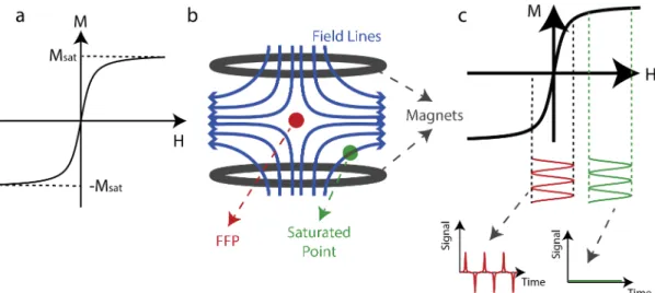
2.1 (a) Characterization of the magnetization, M, of SPIOs as a tion of the aplied field, H, which is governed by a Langevin func-tion. The magnetization of SPIOs saturates beyond a threshold external magnetic field. (b) Schematics of an MPI Scanner. Here blue lines indicate the magnetic field lines, red dot is the field-free-point (FFP), and green dot is an example field-free-point where the SPIO nanoparticles are saturated. (c) When the nanoparticles in the FFP experience a sinusoidal drive field, the time-varying magneti-zation of the nanoparticles induce a signal in the receiver coil, as denoted by red. If the nanoparticles are in the saturated area, their magnetization does not change and hence no signal is induced, as denoted by green. . . 5

2.2 (a) The relaxation mechanisms of the SPIO nanoparticles are il-lustrated. Brownian relaxation occurs when the magnetic moment of the nanoparticles, M, aligns to the applied field, H (red arrow) through a physical rotation (top). On the other hand, Neel relax-ation occurs when the magnetic moment of the nanoparticles aligns to the applied field, H, internally (bottom). (b) The effect of relax-ation on the nanoparticle signal is shown. When the nanoparticle signal has relaxation effect (blue), it is delayed and peak signal is decreased as compared to the nanoparticle signal without any relaxation effect (red). . . 8

LIST OF FIGURES xi

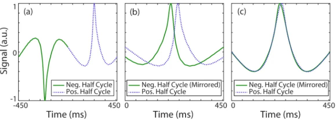
2.3 Estimating the relaxation time constant directly from the mea-sured MPS signal. (a) Meamea-sured MPS signal for nanomag-MIP nanoparticles at 1.1 kHz and 15 mT drive field, for the case of a low viscosity solution (approximately 1.22 mPa·s). The relaxation effect on the signal is clearly visible. (b) The positive half cycle and the mirrored (i.e., time reversed and negated) negative half cycle are overlaid. If the signal had not contained any relaxation effects, these two half cycles would overlap exactly. Due to relaxation, however, each half cycle is blurred along the scanning direction. The time constant estimation yields τ = 32.9 µs. (c) The mea-sured signal can then be deconvolved by the relaxation kernel with the estimated time constant, which reveals the underlying mirror symmetry. . . 10

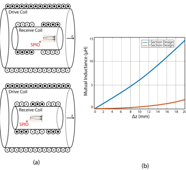
3.1 Mutual inductance comparison between two-section design (a, top) (b, blue) and three-section design (a, bottom) (b, red) when the receive coil is shifted in z direction. Three-section design is more robust in case of any constructional flaws such as off-centered po-sitioning. . . 14

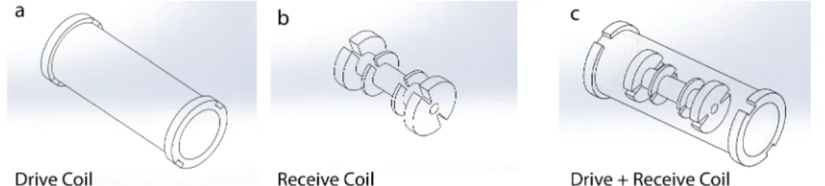
3.2 Solidworks designs of the MPS setup that consists of a drive coil (a) and a receive coil (b). The two coils are coaxially aligned with each other (c). . . 15

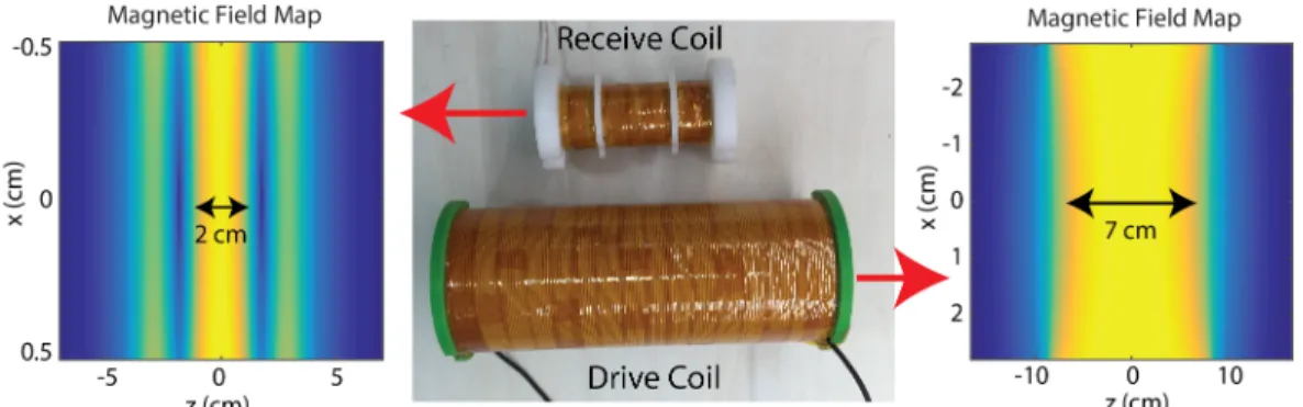
3.3 Magnetic field maps of the custom-made receive and drive coils. The 95% homogeneity occurs in a 7-cm-long region in the drive coil. The receive coil has a 2-cm long sensitive region where it allows a sample tube of 1.5-cm in length. . . 16

3.4 The sensitivities of the drive coil and the receive coil are measured with a Hall effect gaussmeter. 1A DC current is applied to the coils and the measurement point was moved in a stepwise manner using a linear actuator. The measured sensitivities almost perfectly match with the simulation results. . . 16

LIST OF FIGURES xii

3.5 Overview of the experimental setup. Arrows in the schematic de-note the workflow of the transmit/receive chain for my in-house magnetic particle spectrometer (MPS) setup, which is controlled via a data acquisition card (DAQ) through MATLAB. A fiber op-tic thermometer and a current probe provide real-time monitoring of the temperature and the magnetic field in the MPS setup, re-spectively. . . 17

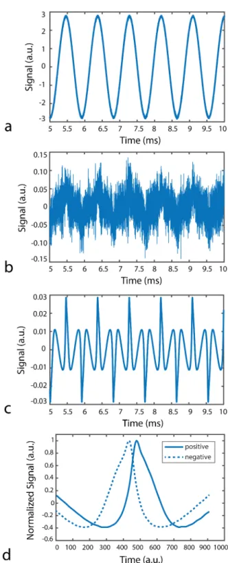
3.6 Acquired data (a) without baseline substraction and (b) with base-line substraction. (c) The resultant signal after choosing the higher harmonics of the drive field frequency in Fourier domain and set-ting all other frequencies to zero. After that a low-pass filter was applied in time domain. (d) An arbitrary period from the signal in (c) is displayed to show that it contains the nanoparticle relaxation effect. The graphs have the same arbitrary unit. . . 20

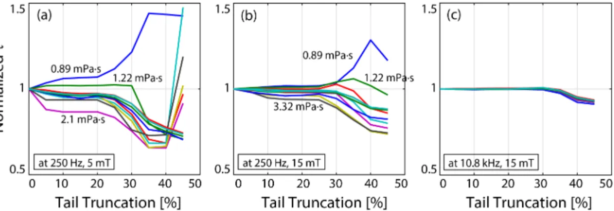
3.7 Influence of tail truncation on the estimated relaxation time con-stants. If the relaxation model worked perfectly, these curves would be horizontally flat, yielding constant τ estimation independent of truncation percentage. At low drive field amplitude and fquency as in (a), large truncation percentage yields diverging re-sults, whereas zero truncation shows a slight variation from the expected flat response. In contrast, at high drive field amplitude and frequency as in (c), the estimations remain constant up to 35% tail truncation. In all cases, tail truncations between 10%-20% yielded constant τ estimations. Results are for nanomag-MIP nanoparticles. . . 22

LIST OF FIGURES xiii

4.1 Effects of viscosity on nanoparticle signal. (a) The measured signal of nanomag-MIP nanoparticles at 1.1 kHz and 15 mT drive field are shown for low viscosity (0.89 mPa·s) and high viscosity (15.33 mPa·s) cases. The low viscosity case displays a wider response with reduced peak amplitude. The calculated relaxation time constant for these two cases were τ = 33µs and τ = 24 µs, respectively. (b) The same samples were measured at 10.8 kHz and 15 mT drive field, yielding τ = 3.5 µs and τ = 3.6 µs, respectively. Here, the high viscosity case has a slightly wider response than the low viscosity case. . . 25

4.2 Relaxation time constants as a function of viscosity, at four differ-ent drive field frequencies for sample set #1 (nanomag-MIP at 11 different viscosities ranging between 0.89 mPa·s to 15.33 mPa·s). Error bars denote the mean values and standard deviations over three repetition experiments. . . 26

4.3 Relaxation time constants as a function of viscosity, at three dif-ferent drive field strengths for sample set #1 (nanomag-MIP at 11 different viscosities ranging between 0.89 mPa·s to 15.33 mPa·s). Error bars denote the mean values and standard deviations over three repetition experiments. (a) to (c) The same data as in Fig. 4.2, re-plotted to emphasize the effect of drive field frequency at a fixed field strength. (d) to (f) The results in a unified y-axis, where the estimated time constants are normalized by the period of the drive field at each frequency, multiplied by 100. . . 28

LIST OF FIGURES xiv

4.4 Relaxation time constant vs. viscosity for the biologically more relevant range of viscosities, for sample set #2 (nanomag-MIP at 20 different viscosities ranging between 0.89 mPa·s to 3.97 mPa·s), measured at four different frequencies at 15 mT field strength. Error bars denote the mean values and standard deviations over three repetition experiments. (a) Estimated time constants and (b) time constants normalized by that of nanoparticles in water to highlight the percentage change in τ vs. viscosity. . . 29

4.5 Effects of viscosity on the relaxation time constants of two dif-ferent nanoparticles. VivoTrax and nanomag-MIP nanoparticles were measured at four different drive field conditions, and at 11 different viscosities ranging between 0.89 mPa·s to 15.33 mPa·s. Error bars denote the mean values and standard deviations over three repetition experiments. . . 30

A.1 Received nanoparticle signal at the viscosity value of 1.22 mPa·s, under the drive field frequency and amplitde of 1.1 kHz and 15 mT. (a) shows the time domain signal and (b) shows the corre-sponding frequency domain of this signal. The direct-feedthrough contamination surpass the nanoparticle signal. Red circle in (b) shows from the 3rd to 13th harmonics of the nanoparticle signal. . 44

A.2 Background signal is substracted from the nanoparticle signal given in Fig. A.1. Now, the direct-feedthrough contamination is highly removed. The nanoparticle harmonics is shown in (b). Also in (b), self-resonance frequency of the receive coil is shown. The self resonance of the receive coil contaminates the higher har-monics of the nanoparticle responce at the drive field frequency of 10.8 kHz. . . 45

LIST OF FIGURES xv

A.3 Once the baseline-substracted signal undergoes a two-stage filter-ing operation, the remainfilter-ing direct-feedthough signal is removed along with the noise in non-harmonic frequencies. The resulting nanoparticle signal shown in (a) has the relaxation effects.(b) shows the frequency domain representation of the time domain signal given in (a). . . 45

Chapter 1

Introduction

Magnetic Particle Imaging (MPI) is a novel imaging modality that was first published in 2005 [1]. MPI utilizes the non-linear magnetization characteris-tics of superparamagnetic (SPIO) nanoparticles to provide spatial localization of nanoparticles. Iron oxide nanoparticles are exploited in MPI as a contrast agent (as opposed to iodine or gadolinium) which makes it a safe imaging method, es-pecially for patients with chronic kidney disease (CKD). MPI has been rapidly developing since it was first published [2, 3, 4] with potential biomedical appli-cations such as angiography [5, 6], stem cell tracking [7, 8, 9], cancer imaging [10], guiding cardiovascular interventions [11], and predicting the effectiveness of magnetic hyperthermia [12, 13]. In MPI, the same pole of two strong magnets face each other to create a zero-field point in between (called the field-free-point, FFP), and this point (FFP) is scanned through the object of interest using a time varying field (drive field). MPI detects the response of SPIO nanoparticles to applied external magnetic fields, without any signal from the background tis-sue. This response is sensitive to the local environment of the SPIOs such as the viscosity of the medium that they are in or their binding state to chemicals, showing a remarkable potential for functional imaging with MPI.

One potential functional imaging application for MPI is in vivo viscosity map-ping. In literature, blood viscosity was shown to change with hematocrit level

[14], and several studies associated high hematocrit levels in the blood plasma with important diseases such as hypertension [15], cerebral infarction [16], angina pectoris [17], ischemic heart disease [18, 19], and extensive coronary artery disease [20]. High blood viscosity levels were also found to be prognostic of certain cancer types [21, 22]. It was further suggested that cancer cells have increased cellular viscosity when compared to healthy cells [23]. Importantly, for cell tracking appli-cations, viscosity in a cell cytoplasm can give information regarding the uptake of external particles into the cell environment as well as activities occurring within the cell. Interactions in the cell environment such as signaling, transportation of molecules, enzymatic activity, binding effect were interrelated with viscosity [24, 25, 26, 27]. Diagnoses of atherosclerosis [28], diabetes [29], Alzheimer’s dis-ease [30], and neurological disorders [31] were found to be related with plasma fluidity, membrane viscosity, and serum viscosity. Given this extensive literature, measuring viscosity in vivo has important diagnostic and prognostic implications, making it a promising functional imaging application for MPI.

The relaxation behaviour of nanoparticles under zero-field (i.e., when an ap-plied magnetic field is removed) is modeled by two different mechanisms: Neel relaxation where the magnetic moment of the nanoparticle aligns itself internally with the applied field, and Brownian relaxation where the nanoparticle physically rotates to align its magnetic moment with the applied field. Extensive simulations showed the influence of particle parameters such as size and shape anisotropy, magnetization dynamics, and the sequence of applied fields [32, 33]. Theoretical modeling for Neel relaxation via Landau-Lifshitz-Gilbert equation and for Brow-nian relaxation via Fokker-Planck equation were also presented [34, 35]. Due to the physical rotation of the nanoparticle, Brownian relaxation is directly influ-enced by the external environment, such as the viscosity of the medium. With this fact in mind, the monitoring of viscosity through the ratio of nanoparti-cle magnetization harmonics was proposed, with potential extensions to system-matrix based MPI reconstruction [36, 37]. The relaxation induced signal delays in x-space based MPI reconstruction were also suggested as a possible tool for es-timating the mobility of nanoparticles [38]. Recent color MPI studies have shown the capability of MPI to separate signals from different nanoparticles [39, 40],

which could in potential be applied to differentiate nanoparticles in different vis-cous environments. In these color MPI techniques, a successful separation relied on extensive calibration acquisitions that essentially characterize the behaviour of the nanoparticles under different settings, or measurements at multiple drive field amplitudes to reveal the differences between the responses of nanoparticles. MPI cell tracking experiments have also shown that nanoparticles internalized into the cells displayed reduced resolution [7] or had altered signal characteristics when compared to nanoparticles in water [9], which could stem from viscosity effects on the relaxation behaviour of the nanoparticles. Hence, understanding the effects of viscosity on MPI signal is vital in developing the viscosity mapping capabilities of MPI for functional imaging purposes.

In this thesis, the viscosity mapping capability of MPI is demonstrated through an estimation of the relaxation induced changes in the nanoparticle response. This estimation does not require any a priori information on the nanoparticles. This functional capability of MPI was verified through a custom-designed magnetic particle spectrometer (MPS) device. Through extensive experiments, the results showed that the relaxation time constant as a function of viscosity is dependent on the drive field strength and frequency. These results provide guidance on MPI imaging parameters that can accentuate the signal differences between nanopar-ticles in environments with different viscosities. The proposed technique can be extended to imaging applications, facilitating the viscosity mapping potential of MPI.

Chapter 2

Background and Theory

2.1

Magnetic Particle Imaging (MPI)

Superparamagnetic iron oxide (SPIO) nanoparticles are utilized as contrast agent in MPI. The magnetization of SPIOs is characterized by a Langevin function where the magnetization saturates beyond a threshold external magnetic field as shown in Fig. 2.1(a). In an MPI scanner, as depicted in Fig. 2.1(b), two magnets create a zero-field point (called field-free point, FFP) in between, and due to the non-zero static field distribution in the remaining points, the nanoparticles are saturated. When the nanoparticles in the FFP experience a sinusoidal drive field, the time-varying magnetization of the nanoparticles induce a signal in the receiver coil. However, if the nanoparticles are in the saturated area, their mag-netization does not change significantly and remain almost constant (i.e., they remain saturated) and hence no signal is induced. The SPIO responses of these points are shown in Fig. 2.1(c).

The static field generated by magnets, which is also called selection field, can be mathematically represented in 1-D as follows:

Hs(x) = −Gx (2.1)

Here G is the selection field gradient strength [T/m/µ0], and x = 0 is the location

Figure 2.1: (a) Characterization of the magnetization, M, of SPIOs as a function of the aplied field, H, which is governed by a Langevin function. The mag-netization of SPIOs saturates beyond a threshold external magnetic field. (b) Schematics of an MPI Scanner. Here blue lines indicate the magnetic field lines, red dot is the field-free-point (FFP), and green dot is an example point where the SPIO nanoparticles are saturated. (c) When the nanoparticles in the FFP experi-ence a sinusoidal drive field, the time-varying magnetization of the nanoparticles induce a signal in the receiver coil, as denoted by red. If the nanoparticles are in the saturated area, their magnetization does not change and hence no signal is induced, as denoted by green.

of FFP. The nanoparticles are excited with a time-varying magnetic field, which is called the drive field, and it is typically in the following form:

Hd(t) = Hpeakcos(2πfdt) (2.2)

where Hpeak [T] is the peak value of the applied sinusoidal field and fd [Hz] is the

frequency of the drive field. The applied magnetic field becomes the summation of the spatial selection field and temporal sinusoidal:

H(x, t) = Hd(t) + Hs(x)

= Hd(t) − Gx

(2.3)

Note that, the location of FFP is at H(x, t) = 0. Solving for the time-dependent position of the FFP, xs(t) in [m] yields:

Hd(t) − Gxs(t) = 0 (2.4)

Hd(t) = Gxs(t) (2.5)

xs(t) =

Hd(t)

G (2.6)

To reconstruct an image from the received signals, there are two main ap-proaches in MPI. One of them is called system-reconstruction method, in which the MPI system is calibrated with a point source before a regular imaging se-quence begins. Alternatively, the other approach is called x-space reconstruction method, in which the nanoparticle responses are directly localized with the knowl-edge of the FFP velocity.

For x-space MPI reconstruction, the 1-D signal equation is derived in [41]. The non-linear magnetization curve of the nanoparticles is described by a Langevin function:

M (H) = mρL[kH] (2.7)

where m [Am2_{] is magnetic moment of the nanoparticle, ρ [particles/m}3_{] is}

density of nanoparticles, k [m/A] is a nanoparticle property, and H = Gx as it

was shown in Eq. 2.1. Assuming the particle distribution is only in x direction, and FFP poisiton is at xs(t), the magnetization can be written as:

M (x, t) = mρ(x)δ(y)δ(z)L[kG(xs(t) − x)] (2.8)

Eq. 2.8 can be converted to magnetic flux as given below. Note that, if we assume ρ changes with only x, this equation is a convolution:

φ(t) = −m Z Z Z

ρ(u)δ(v)δ(w)L[kG(xs(t) − u)] du dv dw

= mρ(x) ∗ L[kGx]|x=xs(t)

(2.9)

Finally, the 1-D MPI signal (also called the adiabatic signal) can be expressed as follows:

sideal(t) = B1

dφ

dt = B1mρ(x) ∗ ˙L[kGx]|x=xs(t)kG ˙xs(t) (2.10)

where B1 [T /A] is receiver coil sensitivity.

2.2

Relaxation in MPI

In practice, the received MPI signal is affected by the relaxation behaviour of the SPIOs. The relaxation causes a peak shift in the MPI signal along with a loss in SNR, which blurs the image. There are two relaxation mechanisms that govern the behaviour of SPIOs when the applied field is removed. First one is called Brownian relaxation, in which the magnetic moment of the nanoparticles aligns externally through a physical rotation. Other mechanism is called Neel relaxation, in which the alignment of the magnetic moment occurs internally to the applied field. The combined effects of these relaxation mechanisms result in a delay of the nanoparticle signal along with decreased peak signal. In Fig. 2.2(a), these two relaxation mechanisms are illustrated, and in Fig. 2.2(b) the effect of relaxation on the nanoparticle signal is shown.

Figure 2.2: (a) The relaxation mechanisms of the SPIO nanoparticles are illus-trated. Brownian relaxation occurs when the magnetic moment of the nanopar-ticles, M, aligns to the applied field, H (red arrow) through a physical rotation (top). On the other hand, Neel relaxation occurs when the magnetic moment of the nanoparticles aligns to the applied field, H, internally (bottom). (b) The effect of relaxation on the nanoparticle signal is shown. When the nanoparticle signal has relaxation effect (blue), it is delayed and peak signal is decreased as compared to the nanoparticle signal without any relaxation effect (red).

The relaxation effect blurs the reconstructed image asymmetrically depending on the scanning direction. Previous studies have modeled this relaxation effect as a temporal convolution of the ideal MPI signal with an exponential relaxation kernel [42, 43]: s(t) = sideal(t) ∗ r(t) (2.11) where, r(t) = 1 τe −t τu(t) (2.12)

Here, τ is called the relaxation time constant and u(t) is the Heaviside step function. It has been verified via extensive experimental work that this phe-nomenological model accurately characterizes the MPI response for a wide range of frequencies and drive field amplitudes [42, 43].

2.3

Direct Estimation of Relaxation Time

Con-stant

In MPI, positive and negative half cycles of the drive field move the FFP forward and back across the scanned partial field-of-view (FOV), repetitively. As a result of this back and forth scanning process, the ideal MPI signal acquired during the positive and the negative scanning directions are mirror symmetric, independent of the nanoparticle distribution ρ(x). Here, mirror symmetry refers to the positive half cycle and the time-reversed and negated negative half cycle of the signal being identical. The ideal half-cycle signals can be expressed as follows:

spos,ideal(t) = −sneg,ideal(−t) = shalf(t) (2.13)

In the case of relaxation, however, the MPI signal is effectively blurred along the scanning direction, which in turn breaks the mirror symmetry between the

two half cycles [44, 45]. To demonstrate this point, Fig. 2.3(a) and Fig. 2.3(b) display the lost mirror symmetry for a measured MPS signal acquired at 1.1 kHz and 15 mT drive field for nanomag-MIP nanoparticles. In theory, the half cycles shown in Fig. 2.3(b) would overlap exactly if the nanoparticles did not exhibit any relaxation behaviour. In theory, the relaxation time constant can be estimated from the half cycles of the MPI signal using the mirror symmetry of the underlying ideal MPI signal, without any a priori information about the nanoparticle type or distribution.

Figure 2.3: Estimating the relaxation time constant directly from the measured MPS signal. (a) Measured MPS signal for nanomag-MIP nanoparticles at 1.1 kHz and 15 mT drive field, for the case of a low viscosity solution (approximately 1.22 mPa·s). The relaxation effect on the signal is clearly visible. (b) The positive half cycle and the mirrored (i.e., time reversed and negated) negative half cycle are overlaid. If the signal had not contained any relaxation effects, these two half cycles would overlap exactly. Due to relaxation, however, each half cycle is blurred along the scanning direction. The time constant estimation yields τ = 32.9µs. (c) The measured signal can then be deconvolved by the relaxation kernel with the estimated time constant, which reveals the underlying mirror symmetry.

Using the convolution-based formulation for the MPI signal, the half cycles in the case of relaxation can be expressed as:

spos(t) = spos,ideal(t) ∗ r(t) = shalf(t) ∗ r(t) (2.14)

sneg(t) = sneg,ideal(t) ∗ r(t) = −shalf(−t) ∗ r(t) (2.15)

Note that shalf(t) is the ideal half-cycle signal. Using the exponential model

for r(t), these two equations can be solved simultaneously to reveal both τ and shalf(t) [44, 45]. Here, the interested variable is the relaxation time constant τ ,

which can be expressed in closed form in the Fourier domain:

F {r(t)} = R(f ) = 1

(1 + i2πf τ ) (2.16)

F {spos(t)} = Spos(f ) = Shalf(f )·R(f ) (2.17)

F {sneg(t)} = Sneg(f ) = −Shalf(−f )·R(f ) (2.18)

Here, Eq. 2.16 is the known 1D Fourier transform of an exponential function and Eq. 2.18 follows from time reversal property of Fourier transform. Since shalf(t) is real valued, its Fourier transform Shalf(f ) has conjugate symmetry

property. Accordingly, the last equation can be re-written as

F {sneg(t)} = Sneg(f ) = −Shalf∗ (f )·R(f ) (2.19)

where the superscript star sign denotes the conjugation operation. Finally, combining Eq. 2.16 to 2.19, the relaxation time constant can be expressed as follows: τ = S ∗ pos(f ) + Sneg(f ) i2πf (S∗ pos(f ) − Sneg(f )) (2.20)

Once this time constant is estimated, the signal can be deconvolved by the relaxation kernel, r(t), to reveal the underlying ideal MPI signal. In theory, this deconvolution step recovers the mirror symmetry between the half cycles. This process is demonstrated in Fig. 2.3(c). In this work, the relaxation time constant

and system delays were estimated simultaneously (see Section 3.4). The τ , φ pair that minimized the RMSE between the deconvolved versions of the positive and the mirrored negative half cycles was chosen as the solution.

Chapter 3

Materials and Methods

3.1

Magnetic Particle Spectrometer Setup

In MPI, the receive coil needs to be in a gradiometer configuration to minimize the mutual inductance between the drive coil and the receive coil. This is because the drive field directly couples into the receive coil and induces a signal that is orders of magnitude larger than the nanoparticle signal. According to our previous simulations, due to the symmetry in the design, an MPS setup that incorporates a three-section receive coil can utilize a shorter drive coil with 23% reduced power consumption to achieve results similar to a design that uses a two-section gradiometer-type receive coil [46]. In a possible constructional flaws, such as off-centered positioning of the receive coil, three-section design is more robust than two-section design. Fig. 3.1 shows the comparison results between these two design types.

In this work, a custom-made magnetic particle spectrometer (MPS) setup (also called an MPI relaxometer) was designed using Solidworks (Dassault Systemes, Canada), which is illustrated in Fig. 3.2. This MPS setup consists of a drive coil that generates 0.97 mT/A magnetic field with 95% homogeneity in a 7-cm-long region down its bore. The drive coil has an inductance of 420µH and an internal

Figure 3.1: Mutual inductance comparison between two-section design (a, top) (b, blue) and three-section design (a, bottom) (b, red) when the receive coil is shifted in z direction. Three-section design is more robust in case of any constructional flaws such as off-centered positioning.

resistance of 2Ω. The inner diameter of the drive coil is 5.6 cm. This MPS setup also utilizes a receive coil which was a three-section gradiometer-type coil that allowed decoupling of the transmit and receive coils [46]. This receive coil design had 7 layers of Litz wire, where each layer contained 41 turns in the middle and 21 turns on both sides. The measurement chamber inside the receive coil allowed a sample tube of 1.5 cm in length and 0.8 cm in diameter. The receive coil has a self-resonance to be around 250 kHz. The magnetic field map simulation for both the drive coil and the receive coil is given in Fig. 3.3.

Figure 3.2: Solidworks designs of the MPS setup that consists of a drive coil (a) and a receive coil (b). The two coils are coaxially aligned with each other (c).

The simulated field maps were also tested with hardware. 1A DC current was applied to the coils via a DC power supply and the magnetic field was measured using a Hall effect gaussmeter (LakeShore 475 DSP Gaussmeter). The probe of gaussmeter was moved in a stepwise manner with an actuator (Velmex, BiSlide). The simulation and experimental result of normalized sensitivities of the drive and receive coils are given in Fig. 3.4. The corresponding sensitivies in this figure are the ones measured in the centerline of the coils (i.e., at r = 0).

The drive coil was impedance matched to an AC power amplifier (AE Techron 7224) using a capacitive network, which enabled maximum transfer to the load while low-pass filtering potential higher harmonics of the drive field. On the re-ceive side, the nanoparticle signal was amplified with a low-noise voltage pream-plifier (Stanford Research Systems SR560). The MPS setup was controlled with an in-house MATLAB script (Mathworks, Natick, MA). A data acquisition card (National Instruments, NI USB-6363) sent the drive field signal to be ampli-fied to the power amplifier and digitized the signal from the receive chain. The drive field amplitude was calibrated via the Hall effect gaussmeter (LakeShore

Figure 3.3: Magnetic field maps of the custom-made receive and drive coils. The 95% homogeneity occurs in a 7-cm-long region in the drive coil. The receive coil has a 2-cm long sensitive region where it allows a sample tube of 1.5-cm in length.

Figure 3.4: The sensitivities of the drive coil and the receive coil are measured with a Hall effect gaussmeter. 1A DC current is applied to the coils and the measurement point was moved in a stepwise manner using a linear actuator. The measured sensitivities almost perfectly match with the simulation results.

475 DSP Gaussmeter) and monitored in real time via a Rogowski current probe (LFR 06/6/300, Power Electronic Measurements Ltd). During the experiments, ambient temperature inside the measurement chamber was monitored using a fiber optic temperature probe (Neoptix Reflex-4). Fig. 3.5 shows the overall experimental configuration.

Figure 3.5: Overview of the experimental setup. Arrows in the schematic denote the workflow of the transmit/receive chain for my in-house magnetic particle spectrometer (MPS) setup, which is controlled via a data acquisition card (DAQ) through MATLAB. A fiber optic thermometer and a current probe provide real-time monitoring of the temperature and the magnetic field in the MPS setup, respectively.

3.2

Viscous Sample Preparation and

Experi-mental Procedures

Viscosity in the cell cytoplasm for an aqueous phase is reported to be around 1-2 mPa·s (close to the 0.89 mPa·s viscosity of pure water at 25◦C), and this number can become larger as the activity inside the cell increases [47]. Viscosity of the blood, on the other hand, is reported to be in the range of 1.3-7.8 mPa·s for hematocrit percentage in the total blood volume ranging between 14 76% [14].

To provide biologically relevant results in light of this information, three different sets of samples were prepared:

Sample Set #1: 11 samples with viscosities ranging between 0.89 mPa·s and 15.33 mPa·s were prepared. The total volume and nanoparticle amount in each sample was kept identical to avoid any Fe concentration bias in the results. Ac-cordingly, each sample contained 50 µL of undiluted nanomag-MIP (Micromod GmbH, Germany) nanoparticles with 89 mmol Fe/L concentration. These sam-ples were then diluted to a total volume of 170 µL, with varying mixtures of deionized water and glycerol to reach the target viscosity levels at 25◦C [48]. Here, 0.89 mPa·s corresponds to the viscosity of pure water, whereas 15.33 mPa·s corresponds to 68% glycerol by volume.

Sample Set #2: To investigate the biological range in more detail, I prepare 20 samples with viscosity levels ranging from 0.89 mPa·s to 3.97 mPa·s following a procedure similar to the one described above. For this second set, the total sample volume was 200 µL, starting from an initial 80 µL volume of undiluted nanomag-MIP nanoparticles. Here, 3.97 mPa·s corresponds to the viscosity of 45% glycerol by volume.

Sample Set #3: To compare the viscosity effect on different nanoparticles, I prepare 11 samples using VivoTrax ferucarbotran nanoparticles (Magnetic Insight Inc., USA) with 98 mmol Fe/L concentration. Note that this nanoparticle has the same chemical composition as Resovist (which is known to have a well MPI response). For this set, same viscosity levels (i.e., ranging from 0.89 mPa·s to 15.33 mPa·s) and volumes were used as in sample set #1

The samples in set #1 were tested at four different drive field frequencies; 250 Hz, 550 Hz, 1.1 kHz, and 10.8 kHz, and under three different drive field peak amplitudes; 5 mT, 10 mT, and 15 mT. The samples in set #2 were tested at the same four frequencies, but only at 15 mT field amplitude. The samples in set #3 were tested at 550 Hz and 1.1 kHz, under two different drive field peak amplitudes: 10 mT and 15 mT. For each experiment, the amplified signal from the receive chain was digitized with 2 MS/s bandwidth. Acquisition lengths were chosen such that each cosine excitation pulse contained at least 35 periods. For

each measurement, the mean of 16 acquisitions were recorded to increase signal-to-noise ratio (SNR). This step was performed first with no sample inside the measurement chamber to serve as the background measurement, and then with the sample. Overall, each experiment was repeated three times.

3.3

Data Preprocessing

Acquired data sets were processed in MATLAB. For each experiment, the back-ground signal was subtracted from the nanoparticle signal to remove the direct feedthrough and other potential interferences. An initial frequency selection was performed by choosing the higher harmonics of the drive field frequency in Fourier domain and setting all other frequencies to zero. This step removed the remain-ing direct feedthrough signal at the fundamental frequency (i.e., drive field fre-quency), as well as the noise in non-harmonic frequencies that would otherwise reduce signal quality. A subsequent high-order zero-phase digital low-pass filter (LPF) was applied in time domain. The cut-off frequency of LPF was determined via comparing the signal power at harmonic frequencies with the noise power at non-harmonic frequencies, which was computed before setting those frequencies to zero. Accordingly, the cut-off frequencies corresponded to 40th, 50th, 50th, and 18th harmonics for 250 Hz, 550 Hz, 1.1 kHz, and 10.8 kHz drive fields, respec-tively. The usage of fewer harmonics at 10.8 kHz was to avoid the self-resonance frequency of the receive coil, which contaminated signals above 200 kHz. The pro-cessing of the received signal is shown in Fig. 3.6. Also the detailed explanation is given in Appendix A.

3.4

Relaxation Time Constant Estimation

The acquired signal contains both the relaxation effects, as well as a phase lag due to inductive/capacitive circuitry. Note that for the ideal MPI signal, the signal peaks would occur at central time points of half cycles, which would trivialize

Figure 3.6: Acquired data (a) without baseline substraction and (b) with baseline substraction. (c) The resultant signal after choosing the higher harmonics of the drive field frequency in Fourier domain and setting all other frequencies to zero. After that a low-pass filter was applied in time domain. (d) An arbitrary period from the signal in (c) is displayed to show that it contains the nanoparticle relaxation effect. The graphs have the same arbitrary unit.

the phase lag estimation. In the case of relaxation, however, the signal peaks are inherently delayed in time with respect to the half-cycle centers.

Here, the relaxation time constant and the system delays were estimated simul-taneously from the received signal, without any prior information. Accordingly, a sweep of phase lags, φ, between 0 and π were applied to the received signal and the signal was divided into positive/negative half cycles for each phase lag case. The relaxation time constant, τ , was estimated from these half cycles as described in Subsection 2.3. The signal was then Wiener deconvolved by the relaxation kernel r(t) given in Eq. 2.12. A necessary condition for the successful imple-mentation of the deconvolution step is to have sufficiently high SNR [49], which was achieved via the data processing steps outlined in Subsection 2.3. Next, the root-mean-squared error (RMSE) between the deconvolved positive half cycle, ˆ

s(pos,ideal), and mirrored negative half cycle, ˆs(neg,ideal,mirr), was computed. This

step was to check whether the mirror symmetry was restored after deconvolution. Finally, the {τ , φ} pair that minimized RMSE was chosen as the solution, i.e.,

{ˆτ , ˆφ} = argmin{τ,φ}

Z

|ˆspos,ideal(t) − ˆsneg,ideal(t)|2dt (3.1)

The restoration of mirror symmetry via this technique was confirmed via visual inspection of results on randomly selected experimental data. The tails of the half cycles were excluded from the RMSE calculation step, as they corresponded to the lowest SNR regions of the signal. Accordingly, 15% of the signal was cut from both sides of the half cycles during RMSE calculation. This choice is further explained in Section 3.5. Finally, as each experiment had three repetitions, the mean value and standard deviations across these repetitions were computed for each viscosity level at each drive field strength and frequency.

3.5

Influence of Tail Truncation on Estimated

Time Constants

The model in Eq. 2.11 and 2.12 is phenomenological, i.e., it is based on extensive experimental work that demonstrates a good fit to this model [42]. If this model could mimic the relaxation behaviour perfectly, deconvolution with the correct relaxation kernel would restore mirror symmetry completely. As shown in Fig. 2.3(c), the half cycles after deconvolution display close to perfect mirror sym-metry, notwithstanding a small region of mismatch at the signal peak locations. The mismatch in the peaks could be avoided by assigning more weight to the goodness-of-fit at the center of half cycles. Doing so, however, would worsen the overlap in the remaining portions of the half cycles.

Figure 3.7: Influence of tail truncation on the estimated relaxation time constants. If the relaxation model worked perfectly, these curves would be horizontally flat, yielding constant τ estimation independent of truncation percentage. At low drive field amplitude and frequency as in (a), large truncation percentage yields diverging results, whereas zero truncation shows a slight variation from the ex-pected flat response. In contrast, at high drive field amplitude and frequency as in (c), the estimations remain constant up to 35% tail truncation. In all cases, tail truncations between 10%-20% yielded constant τ estimations. Results are for nanomag-MIP nanoparticles.

The influence of truncating different percentages of the deconvolved half-cycle tails during RMSE calculations wa analyzed. For example, when 100% of the half cycles are utilized (i.e., 0% truncation), the RMSE calculation takes into account the overlap of both the tails and the center of the half cycle. Alternatively, one

can truncate a percentage of the tails before calculating the RMSE, such that the overlap of the central regions becomes the main target. Fig. 3.7 shows the effect of tail truncation percentage on the estimated relaxation time constants. The values are normalized to show the overall trends. Here, a 10% truncation indicates 10% of half cycles truncated from both tails, with the remaining central 80% utilized in RMSE calculation. If the relaxation model worked perfectly, one would expect to see a flat τ vs. truncation percent curve, i.e., estimated τ would be independent of the truncation percentage. This is in fact the case at high frequency and high field amplitude, as seen in Fig. 3.7(c). At low frequencies and low field amplitudes, however, a large truncation percentage yields diverging results. These results indicate that the exponential model is a better fit at high drive field frequencies and amplitudes. In all cases considered in this work, estimation remained flat for truncation percentages ranging between 10% and 20%. Accordingly, a truncation percentage of 15% was utilized in all τ estimations presented in this work.

Chapter 4

Results

Overall, 768 distinct experiments were performed. For sample set #1, nanomag-MIP nanoparticles at 11 viscosity levels were measured at 3 different field strengths, at 4 different frequencies, and with 3 repetitions (396 experiments). For sample set #2, nanomag-MIP nanoparticles at 20 viscosity levels were mea-sured at a single field strength, at 4 different frequencies, and with 3 repetitions (240 experiments). For sample set #3, VivoTrax nanoparticles at 11 viscosity levels were measured at 2 different field strengths, at 2 different frequencies, and with 3 repetitions (132 experiments).

4.1

Effect of Viscosity on MPS Signal

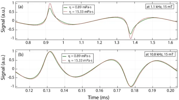
First, the effects of viscosity on the MPS signal were investigated at different drive field amplitudes and frequencies. Fig. 4.1(a) compares two cases of MPS signals: at viscosity levels of 0.89 mPa·s (nanoparticles in water) and 15.33 mPa·s (nanoparticles in water/glycerol mixture of 68% glycerol by volume), both ac-quired at 1.1 kHz and 15 mT drive field. Considering that both samples had the same iron content, one can note that the signal at low viscosity level is re-duced when compared to that at high viscosity. In addition, the response at low

viscosity is visibly wider, indicating an increased relaxation time constant. The estimated time constants were τ = 33µs and τ = 24 µs for η = 0.89 mPa·s and η = 15.33 mPa·s, respectively. Fig. 4.1(b) compares the same samples at 10.8 kHz and 15 mT drive field. This time, in contrast to the results at 1.1 kHz, the signal at high viscosity is slightly wider than the one at low viscosity. The estimated times constants were τ = 3.5µs and τ = 3.6 µs for η = 0.89 mPa·s and η = 15.33 mPa·s, respectively.

Figure 4.1: Effects of viscosity on nanoparticle signal. (a) The measured signal of nanomag-MIP nanoparticles at 1.1 kHz and 15 mT drive field are shown for low viscosity (0.89 mPa·s) and high viscosity (15.33 mPa·s) cases. The low viscosity case displays a wider response with reduced peak amplitude. The calculated relaxation time constant for these two cases were τ = 33 µs and τ = 24 µs, respectively. (b) The same samples were measured at 10.8 kHz and 15 mT drive field, yielding τ = 3.5 µs and τ = 3.6 µs, respectively. Here, the high viscosity case has a slightly wider response than the low viscosity case.

4.2

Effect of Drive Field Amplitude

The relaxation times constants were estimated for all MPS signals acquired. The results for sample set #1 (with 11 different viscosity levels) at four different drive field frequencies and three different drive field strengths are presented in Fig. 4.2

and Fig. 4.3. Error bars denote the mean estimated time constants and standard deviations over three repetition experiments. In Fig. 4.2, for fixed frequency, estimated time constants decrease as field strength increases. The relaxation time constant as a function of viscosity displays a non-monotonic trend. Especially at low drive field frequencies and amplitudes (e.g., at 250 Hz and 5 mT), τ first increases sharply and then decreases with increasing viscosity, finally converging to a roughly constant value. At 10.8 kHz, on the other hand, τ slowly but steadily increases with increasing viscosity.

Figure 4.2: Relaxation time constants as a function of viscosity, at four different drive field frequencies for sample set #1 (nanomag-MIP at 11 different viscosities ranging between 0.89 mPa·s to 15.33 mPa·s). Error bars denote the mean values and standard deviations over three repetition experiments.

4.3

Effect of Drive Field Frequency

In Fig. 4.3, the same data are re-plotted, this time to highlight the effect of drive field frequency on estimated time constants. In Fig. 4.3(a) to 4.3(c), the time constants decrease with increasing frequency. Interestingly, one can see that there is a global trend in these curves, such that the same τ vs. viscosity curve is scaled down and shifted towards the left as frequency increases. Fig. 4.3(d) to 4.3(f) present these results with a normalized time axis, where the estimated time constants are normalized by the period of the drive field at each frequency, and multiplied by 100. Effectively, this unified y-axis gives an indication of the percentage effect of relaxation delays at each frequency. Overall, for fixed drive field amplitude, the relaxation effects are more prominent at higher frequencies. Exceptions to this trend are low viscosity and low drive field strengths, where the trends can be reversed (e.g., at 5 mT for viscosities lower than 3 mPa·s).

To investigate the biologically more relevant viscosities of up to 4 mPa·s, the time constants for sample set #2 with 20 different viscosity levels between 0.89 mPa·s and 4 mPa·s were estimated at four different drive field frequencies with 15 mT field strength. Another motivation for this second set of experiments was to ensure that the τ vs. viscosity curves did not exhibit erratic jumps with a slight variation in viscosity. The results given in Fig. 4.4(a) are consistent with the low viscosity portions of the results in Fig. 4.3(c), as no erratic behaviour is observed. Note that the estimated time constantsat 2.5 mPa·s and 3.6 mPa·s showed slight deviations from the overall trends. These deviations could stem from pipetting errors during the mixing of water and glycerol, as a small variation in glycerol percentage can significantly alter the viscosity level of the mixture. In Fig. 4.4(b), the relaxation time constants are normalized by that of nanoparticles in water (i.e., the lowest viscosity of 0.89 mPa·s), so that the percentage change in τ can be visualized. At 250 Hz, τ first increases by 40% at around 2.2 mPa·s, then gradually decreases. At 1.1 kHz, τ monotonically decreases, showing a 32% reduction at around 4 mPa·s. At 10.8 kHz, on the other hand, τ increases by only 2% within this viscosity range.

Figure 4.3: Relaxation time constants as a function of viscosity, at three different drive field strengths for sample set #1 (nanomag-MIP at 11 different viscosities ranging between 0.89 mPa·s to 15.33 mPa·s). Error bars denote the mean values and standard deviations over three repetition experiments. (a) to (c) The same data as in Fig. 4.2, re-plotted to emphasize the effect of drive field frequency at a fixed field strength. (d) to (f) The results in a unified y-axis, where the estimated time constants are normalized by the period of the drive field at each frequency, multiplied by 100.

Figure 4.4: Relaxation time constant vs. viscosity for the biologically more rel-evant range of viscosities, for sample set #2 (nanomag-MIP at 20 different vis-cosities ranging between 0.89 mPa·s to 3.97 mPa·s), measured at four different frequencies at 15 mT field strength. Error bars denote the mean values and stan-dard deviations over three repetition experiments. (a) Estimated time constants and (b) time constants normalized by that of nanoparticles in water to highlight the percentage change in τ vs. viscosity.

4.4

Comparison of Different Nanoparticles

To provide a better understanding of the effects of viscosity on different nanopar-ticles, experiments were performed with VivoTrax nanoparticles at 11 different viscosity levels (sample set#3). The results are given in Fig. 4.5, in comparison with nanomag-MIP nanoparticles under the same drive field conditions. Ac-cordingly, the estimated time constants for VivoTrax are larger than those for nanomag-MIP, in general. Importantly, the relaxation time constants for Vivo-Trax display a non-monotonic trend as a function of viscosity, as was the case for nanomag-MIP. Furthermore, the global trend seen in nanomag-MIP is also observed for VivoTrax: the same τ vs. viscosity curve is scaled down and shifted towards the left with increasing frequency, as can be seen comparing Fig. 4.5(a) with 4.5(c).

During all experiments, the ambient temperature inside the measurement chamber remained between 23-36◦C, which corresponds to a minor 4% variation

Figure 4.5: Effects of viscosity on the relaxation time constants of two different nanoparticles. VivoTrax and nanomag-MIP nanoparticles were measured at four different drive field conditions, and at 11 different viscosities ranging between 0.89 mPa·s to 15.33 mPa·s. Error bars denote the mean values and standard deviations over three repetition experiments.

in absolute temperature in Kelvins. This variation was due to resistive heating of the drive coil under currents reaching 22 A, which causes a power dissipation of about 350 Watts. Nonetheless, during signal acquisition, each sample tube stayed in the measurement chamber for only 5 seconds at a time. In a separate control experiment, we also measured the temperature inside the sample tubes for the case when the chamber temperature was at 36◦C. Accordingly, during the 5-second interval that the sample was exposed to convective heat transfer, its temperature only changed by 0.3-0.4◦C. Hence, we do not expect any temperature bias for the results reported in this work.

Chapter 5

Discussion and Conclusion

Viscosity sensing is currently infeasible with ultrasound, magnetic resonance imaging, or other preclinical imaging techniques. This work demonstrated the potential of MPI for viscosity mapping through the estimation of the nanopar-ticle relaxation time constant. As shown in the results in Fig. 4.2 to 4.4, the trend in the τ vs. viscosity curves strongly depend on the drive field strength and frequency. Ideally, a quantitative viscosity mapping technique should provide a one-to-one mapping of the measured parameter to the viscosity level. Such a technique should also show a sufficiently large variation of the measured parame-ter as a function of viscosity, such that the viscosity can be deparame-termined accurately. For the biologically relevant range investigated in Fig. 4.4, these requirements are best satisfied by the measurements at 1.1 kHz, where the relaxation time con-stant monotonically decreases with increasing viscosity and displays greater than 30% variation. At 10.8 kHz, on the other hand, the time constant remains almost constant at different viscosity levels. These findings imply that the regular MPI operating frequencies of 25 kHz or 150 kHz are not optimal for viscosity mapping purposes. For the very low drive field frequencies around 250 Hz, on the other hand, τ is a non-monotonic function of viscosity, which would create an ambigu-ity in viscosambigu-ity mapping. A potential solution at those frequencies could be to perform measurements at two different field strengths to determine the viscosity level.

The well-known Brownian relaxation time constant of nanoparticles is given as τ = 3Vη/kBT, where the time constant increases linearly with viscosity, which

is clearly not the case for the results shown in this work. It should be empha-sized that the Neel and Brownian time constants are valid for the zero field case only, i.e., when an applied external magnetic field is suddenly removed. Hence, they do not model the more complex cases such as a sinusoidal external field. For those cases, simulation results solving Landau-Lifshitz-Gilbert equation or Fokker-Planck equation were presented [34, 35]. A previous method considered a dynamic magnetization model, where the ratio of 5th to 3rd harmonics of nanoparticle magnetization was utilized to probe viscosity. Accordingly, a non-monotonic trend was observed as a function of viscosity, both in simulations as well as in experiments with Feridex in various gelatin concentrations [36]. Here, the relaxation time constant in Eq. 2.11 and Eq. 2.12 is a lumped parameter that models the blurring effect in the time-domain MPI signal, without considering the underlying physical mechanisms. Still, the result in Fig. 4.1(a) that displays a visibly narrower response at higher viscosity level is counter intuitive, as one would expect a slower nanoparticle response with increasing viscosity. This could potentially be due to the chemical differences between the water solution vs. the high viscosity water/glycerol mixture, which can potentially affect the interac-tion of the nanoparticles with each other and with the medium. Experiments in solutions with similar viscosities but with different chemical properties could help in understanding this effect.

Previous studies have demonstrated that the MPI signal properties strongly depend on the nanoparticle type [50]. The experiments here were performed using nanomag-MIP and VivoTrax, where both nanoparticles displayed similar non-monotonic trends. Interestingly, the response of VivoTrax at 1.1 kHz and 10 mT was very similar to the response of nanomag-MIP at 550 Hz and 15 mT, as can be seen in Fig. 4.5. These similarities imply that the same physical mechanism is taking place for both nanoparticles, albeit at different strengths. It should be noted that both of these nanoparticles are multi-core nanoparticles with clusters made up of smaller nanoparticles [51]. It remains to be shown whether similar trends are valid for single-core nanoparticles with large diameters.

One important factor to take into account during viscosity mapping with the proposed technique is the homogeneity of the drive field. As seen in Fig. 4.2, for a fixed frequency, changes in drive field amplitude significantly change the estimated relaxation time constant. Hence, to ensure a quantitative mapping of the viscosity during 3D imaging applications, either the drive field needs to be highly homogeneous within the field-of-view (FOV), or one needs to know the field map within the FOV. Another important consideration is the human safety limits of the applied drive fields [52, 53, 54]. According to the results shown in this work, frequencies around 1 kHz have the potential to provide a one-to-one viscosity mapping capability. For 1 kHz, the magnetostimulation safety limit in the human torso can roughly be estimated as 20 mT peak [52]. Hence, the results presented at 1.1 kHz and 15 mT-peak field strength are actually applicable according to the human safety limits of MPI. It should be noted that operating at a lower frequency than the current MPI frequencies (25 kHz, or lately 150 kHz) would have both advantages and disadvantages in terms of image quality. Previous work has shown that peak signal values changed approximately linearly with the drive field frequency and amplitude [55, 43]. Similarly, in our experiments, the received signal strength (before the low-noise preamplifier) at 1.1 kHz was around 10 times lower than that at 10.8 kHz for the same drive field amplitude (results not shown). Hence, the image SNR would decrease when operating at lower frequencies. On the other hand, lower drive field frequencies could yield better resolution images, as previously demonstrated via resolution measurements in a relaxometer setup [43]. Likewise in our experiments, the nanoparticle signal at 1.1 kHz had a narrower peak than that at 10.8 kHz for the same drive field amplitude, as seen in Fig. 4.1.

At all frequencies tested in this work, the relaxation time constants showed an asymptotic convergence for viscosity levels above 5 mPa·s, remaining almost flat above 8 mPa·s. These results indicate that viscosity mapping with this tech-nique may not be feasible at very high viscosity levels. However, there is good evidence in the literature that viscosities below 5 mPa·s are biologically more relevant. For example, it has been previously reported that hematocrit level

exceeding 46% (> 2.8 mPa·s) is considered as an important risk factor for cere-bral infarction, atherosclerosis in the arteries, and hypertension [16]. In another study, elevated viscosity levels from 1.48 mPa·s to 1.71 mPa·s due to myocardial infarction was reported [18]. These viscosity levels are within the mapping capa-bilities of the proposed technique, demonstrating the potential of MPI imaging to provide critical functional information.

To conclude this thesis, the viscosity mapping capability of MPI was demon-strated through proof-of-concept experiments in an MPS device. The technique used to correlate viscosity with the relaxation time constant takes advantage of the underlying mirror symmetry in the time-domain MPI signal. The experimen-tal results at various drive field frequencies suggest that a relatively low drive field frequency of around 1 kHz is promising for a one-to-one viscosity mapping. Future imaging applications exploiting the MPI signals dependence on local vis-cosity of the nanoparticles will benefit from the results provided in this work.

Bibliography

[1] B. Gleich and J. Weizenecker, “Tomographic imaging using the nonlinear response of magnetic particles.,” Nature, vol. 435, pp. 1214–7, jun 2005. [2] P. W. Goodwill, E. U. Saritas, L. R. Croft, T. N. Kim, K. M. Krishnan,

D. V. Schaffer, and S. M. Conolly, “X-Space MPI: Magnetic Nanoparticles for Safe Medical Imaging,” Advanced Materials, vol. 24, pp. 3870–3877, jul 2012.

[3] E. U. Saritas, P. W. Goodwill, L. R. Croft, J. J. Konkle, K. Lu, B. Zheng, and S. M. Conolly, “Magnetic particle imaging (MPI) for NMR and MRI researchers.,” Journal of magnetic resonance (San Diego, Calif. : 1997), vol. 229, pp. 116–26, apr 2013.

[4] L. M. Bauer, S. F. Situ, M. A. Griswold, and A. C. S. Samia, “Magnetic Particle Imaging Tracers: State-of-the-Art and Future Directions,” Journal of Physical Chemistry Letters, vol. 6, pp. 2509–2517, jul 2015.

[5] J. Weizenecker, B. Gleich, J. Rahmer, H. Dahnke, and J. Borgert, “Three-dimensional real-time in vivo magnetic particle imaging.,” mar 2009.

[6] K. Lu, P. W. Goodwill, E. U. Saritas, B. Zheng, and S. M. Conolly, “Linear-ity and shift invariance for quantitative magnetic particle imaging.,” IEEE transactions on medical imaging, vol. 32, pp. 1565–1575, sep 2013.

[7] B. Zheng, T. Vazin, P. W. Goodwill, A. Conway, A. Verma, E. U. Saritas, D. Schaffer, and S. M. Conolly, “Magnetic Particle Imaging tracks the long-term fate of in vivo neural cell implants with high image contrast,” Sci Rep, vol. 5, p. 14055, 2015.

[8] B. Zheng, M. P. von See, E. Yu, B. Gunel, K. Lu, T. Vazin, D. V. Schaffer, P. W. Goodwill, and S. M. Conolly, “Quantitative Magnetic Particle Imaging Monitors the Transplantation, Biodistribution, and Clearance of Stem Cells In Vivo,” Theranostics, vol. 6, no. 3, pp. 291–301, 2016.

[9] K. Them, J. Salamon, P. Szwargulski, S. Sequeira, M. G. Kaul, C. Lange, H. Ittrich, and T. Knopp, “Increasing the sensitivity for stem cell monitoring in system-function based magnetic particle imaging,” Phys Med Biol, vol. 61, no. 9, pp. 3279–3290, 2016.

[10] E. Yu, M. Bishop, P. W. Goodwill, B. Zheng, M. Ferguson, K. M. Krishnan, and S. M. Conolly, “First Murine in vivo Cancer Imaging with MPI,” in 6th International Workshop on Magnetic Particle Imaging (IWMPI), p. 148, 2016.

[11] J. Haegele, J. Rahmer, B. Gleich, J. Borgert, H. Wojtczyk, N. Panagiotopou-los, T. M. Buzug, J. Barkhausen, and F. M. Vogt, “Magnetic particle imag-ing: visualization of instruments for cardiovascular intervention.,” Radiology, vol. 265, pp. 933–938, dec 2012.

[12] K. Murase, M. Aoki, N. Banura, K. Nishimoto, A. Mimura, T. Kubayabu, and I. Yabata, “Usefulness of Magnetic Particle Imaging for Predicting the Therapeutic Effect of Magnetic Hyperthermia,” Open Journal on Medical Imaging, vol. 5, no. June, pp. 85–99, 2015.

[13] D. Hensley, P. Goodwill, R. Dhavalikar, Z. W. Tay, B. Zheng, C. Rinaldi, and S. M. Conolly, “Imaging and Localized Nanoparticle Heating with MPI,” in 6th Int. Workshop on Magnetic Particle Imaging (IWMPI), p. 171, 2016.

[14] B. Pirofsky, “The determination of blood viscosity in man by a method based on Poiseuille’s law,” J Clin Invest, vol. 32, no. 4, pp. 292–298, 1953.

[15] G. Tibblin, S. E. Bergentz, J. Bjure, and L. Wilhelmsen, “Hematocrit, plasma protein, plasma volume, and viscosity in early hypertensive disease,” Am Heart J, vol. 72, no. 2, pp. 165–176, 1966.

[16] H. Tohgi, H. Yamanouchi, M. Murakami, and M. Kameyama, “Importance of the hematocrit as a risk factor in cerebral infarction,” Stroke, vol. 9, no. 4, pp. 369–374, 1978.

[17] G. E. Burch and N. P. Depasquale, “Hematocrit, Viscosity and Coronary Blood Flow* *Supported by grants from the U.S. Public Health Service.,” Diseases of the Chest, vol. 48, no. 3, pp. 225–232, 1965.

[18] J. Fuchs, A. Pinhas, E. Davidson, Z. Rotenberg, J. Agmon, and I. Wein-berger, “Plasma viscosity, fibrinogen and haematocrit in the course of un-stable angina.,” Eur Heart J, vol. 11, no. 11, pp. 1029–1032, 1990.

[19] J. Fuchs, I. Weinberger, Z. Rotenberg, A. Erdberg, E. Davidson, H. Joshua, and J. Agmon, “Plasma viscosity in ischemic heart disease,” Am Heart J, vol. 108, no. 3 Pt 1, pp. 435–439, 1984.

[20] G. D. Lowe, M. M. Drummond, A. R. Lorimer, I. Hutton, C. D. Forbes, C. R. Prentice, and J. C. Barbenel, “Relation between extent of coronary artery disease and blood viscosity.,” Bmj, vol. 280, no. 6215, pp. 673–674, 1980.

[21] G. F. von Tempelhoff, N. Schonmann, L. Heilmann, K. Pollow, and G. Hom-mel, “Prognostic role of plasmaviscosity in breast cancer,” Clin Hemorheol Microcirc, vol. 26, no. 1, pp. 55–61, 2002.

[22] W. L. Chandler and G. Schmer, “Evaluation of a new dynamic viscometer for measuring the viscosity of whole blood and plasma,” Clin Chem, vol. 32, no. 3, pp. 505–507, 1986.

[23] M. F. Guyer and P. E. Claus, “Increased Viscosity of Cells of Induced Tu-mors,” Cancer Research, vol. 2, pp. 16–18, jan 1942.

[24] S. P. Williams, P. M. Haggie, and K. M. Brindle, “19F NMR measurements of the rotational mobility of proteins in vivo.,” Biophysical journal, vol. 72, no. 1, pp. 490–8, 1997.