Improving the accuracy of a time lens
Vladimir B. YurchenkoDepartment of Electrical and Electronics Engineering, Bilkent University, Bilkent, Ankara TR-06533, Turkey, and Institute of Radiophysics and Electronics, National Academy of Sciences of Ukraine,
12 Proskura Street, Kharkov 310085, Ukraine
Received February 11, 1997; revised manuscript received July 22, 1997
A method for improving the accuracy of temporal imaging with an imperfect time lens is proposed. Signal distortion arising from complicated dispersion of the delay lines can be reduced considerably by appropriate choice of the phase-modulation function including the second harmonic of the basic modulation frequency and a specific phase shift of the modulation with respect to the main signal. The method is of particular interest for picosecond and femtosecond optical pulse generation. © 1997 Optical Society of America
[S0740-3224(97)05211-9]
1. INTRODUCTION
Recently there has been considerable interest in temporal imaging with a time lens.1–3 A time lens can stretch and compress signals in time by varying phase relations among various components of their spectra.1 The idea of transforming signal spectra to resolve and compress sig-nals was introduced in radiophysics4and later developed in optics with the purpose of generating ultrashort laser pulses.5–8
The action of the time lens has been thoroughly treated by Kolner and Nazarathy1and by Kolner.2,3 It is based
on the analogy between the propagation of a wave packet in a dispersive medium and the diffraction of a beam in free space. Spatial imaging with a glass lens involves diffraction from object to lens, a spatially dependent phase shift provided by the lens, and diffraction from the lens to an image. Similarly, temporal imaging with a time lens requires dispersion from an object pulse to the lens, a time varying phase shift that is due to the lens, and dispersion from the lens to an image pulse. Hence the entire time lens system consists of two dispersive el-ements (delay lines) and a phase modulator between them (the time lens itself ). In the research reported in Refs. 7 and 8, dispersive elements were realized by grat-ing pairs, and the optical phase modulator was composed of a LiNbO3crystal placed in a waveguide with the phase
velocity of the driving microwave mode matched to that of the optical wave in the crystal. Similarly to its spatial counterpart, the time lens can rescale temporal signals, preserving their shape, when some special tuning condi-tions are satisfied (see below).
The time lens is perfect when the phase shift that arises in the dispersive lines is quadratic in frequency and the phase modulation is quadratic in time. In this case, the initial signal is scaled in time, with no distortion if the parameters of the functionsb (v) and w(t), where b is the propagation constant,v is the frequency, w is the phase modulation, and t is the time, are matched accord-ing to the equation of a lens.1,2 This is the case that was carefully studied in previous papers.1–3
In practice, the time lens is not perfect because the
phase modulation is normally sinusoidal7,8and the dis-persion law is not exactly quadratic. Therefore some sig-nal distortion is inevitable and is often more significant than the regular nonparaxial effects in the spatial lens. In the time lens, however, there is a possibility of control-ling not only the phase modulation w(t) but both func-tionsw(t) andb (v) simultaneously. In this way one can try to adjust the functions properly to decrease signal dis-tortion to a minimum even when both of them are not quadratic.
We propose a method for improving the accuracy of temporal imaging with an imperfect time lens by opti-mum choice of phase modulation adjusted to the given nonquadratic dispersion of the delay lines used in the sys-tem.
2. FORMULATION
In the dispersive medium the wave equation for the elec-tric field E(t, z) is of the form
]2E~t, z! ]z2 2 1 c2 ]2 ]t2
E
0 ` «r~t!E~t 2 t, z!dt 5 0, (1) where «r(t) is the relative dielectric function of the me-dium and c is the speed of light in free space. One can find an analytical solution to Eq. (1) by using the Laplace transform, which is the most suitable method for the given problem.9 In terms of the envelope of the wavepacket E(t, z)5 U(t, z)exp$i@v0t2b (v0)z#% at the
car-rier frequencyv0, the solution is
U1~u, z! 5
E
2``
U0~t!G~u 2 t, z!dt, (2)
where U0(t)5 U(t, 0) is the input signal, U1(u, z) is the
signal at a distance z, u 5 t12 z/vg, vgis the group ve-locity at frequency v0, G(u 2 t, z) is the Green’s
func-tion given by the integral
G 5 1
2p
E
2``
exp$i@~u 2 t!~v 2 v0! 2 G~v!z#%dv,
(3)
Vladimir B. Yurchenko Vol. 14, No. 11 / November 1997 / J. Opt. Soc. Am. B 2921
G(v) 5b(v) 2 b02 b1(v 2 v0), b2(v) 5 «r(v)v2/c2, «r(v) is the Fourier transform of the dielectric function «r(t), b05b(v0), andb15 1/vg5]b(v)/]vuv5v0.
In the third-order approximation, when
b~v! 5 b01 b1~v 2 v0! 11/2b2~v 2 v0!2 1 1/6b 3~v 2 v0!3, (4) one has G5 G3~u 2 t, z! 5 1 2p
E
2` ` exp$i@~u 2 t!v 21/2b 2zv2 21/6b 3zv3#%dv. (5)In the second order, whenb35 0, G(u 2 t, z) is
simpli-fied to
G 5 G2~u 2 t, z! 5 ~2pib2z!21/2exp@i~u 2 t!2/2b2z#,
(6) providing an exactly quadratic phase shift in the fre-quency domain.
Consider now the action of the time lens. Suppose that the dispersive lines are of lengths L1 and L2, and
that the phase modulator transforms the signal
U1(u, L1) as
U2~u, L1! 5 U1~u, L1!exp@iw~u!#, (7)
where w(u) 5 w01w1u 1 w2u21w3u3 in the
third-order approximation. Then the output signal U3(t) at
the end of the system is given by the relation
U3~t! 5
E
2` ` dtU0~t!E
2` ` duG~t 2 u, L2! 3 exp@iw~u!#G~u 2 t, L1!, (8) wheret 5 u 2 (z 2 L1)/vg.When G5 G2 and the phase modulation is quadratic,
w(u) 5 w2u2, one obtains
U3~t! 5 2 i b2
A
L1L2 expS
it 2 2b2L2D
E
2` ` dtU0~t!I~t, t! 3 expS
it 2 2b2L1D
, (9) where I~t, t! 5 21pE
2` ` du expF
iu2S
1 2b2L2 1 w21 1 2b2L1DG
3 expF
2 i bu 2S
t L2 1 t L1DG
. (10)In this case, under the condition that
1/~2b2L2! 1 1/~2b2L1! 1w25 0, (11)
which is the regular equation of a lens,1 one has I(t, t) 5 b2L1d(t 1tL1/L2) and obtains the well-known
result10that the output signal U3(t) is of the same form
as the input signal but of a different time scale, i.e.,
U3~t! 5 2i
S
L1 L2D
1/2 expS
it2 L11 L2 2b2L22D
U0S
2 L1 L2 tD
, (12)where the scaling factor is K(0)5 2L
1/L2(the phase
fac-tor is not essential).
When the dispersion lawb (v) and the phase modula-tionw (u) are not quadratic, the inner integral in the gen-eral formula [Eq. (8)] is not simplified to the dfunction. Therefore, in this case, the output signal U3(t) is no
longer similar to U0(t). The exact analysis of the
trans-form is rather complicated, even in the third-order ap-proximation, when G5 G3 according to Eq. (5).
How-ever, if one takes G3 as
G35 G3~u 2 t, z! 5 A~u 2 t, z!exp@iF~u 2 t, z!#,
(13) and makes a notion that, in the given phenomenon, varia-tion of the phase factor F(u 2 t, z) compared with A(u 2 t, z) is more essential, an approximate analysis is pos-sible.
Equation (13) arises naturally if the stationary-phase asymptotic evaluation of integral (5) is performed. If a few points of the stationary phase exist (e.g., two, as for the function G3), one can for simplicity take into account
only one of them, which relates to the minimum oscilla-tions in function (13) to yield the main contribution to in-tegral (8).
Let us expand phase function Fi(i5 1, 2 refers to the first or the second dispersion line, respectively) in the power series in u 2 t (or t 2 u) with descending coeffi-cients fik. When i 5 1, one has, for example, F1(u
2 t, L1)5 f101 f11(u 2 t) 1 f12(u 2 t)21 f13(u 2 t)3,
where the third-order approximation is used. Then Eq. (8) takes the form
U3~t! 5
E
2` ` dtU0~t!E
2` ` duC~u, t, t!exp@iS~u, t, t!#, (14) where S~u, t, t! 5 u@~ f112 f211 w1! 2 2~ f12t1 f22t! 1 3~ f13t22 f23t2!# 1u2@~ f121 f221w2! 2 3~ f13t2 f23t!# 1 u3@ f132 f231 w3#. (15) If the stationary-phase method that accounts for one stationary point is applied to Eq. (5), the coefficients fik are found approximately as fi15 0, fi25 1/(2b2Li), andfi35b3/(6b22Li2). Analysis shows, however, that for accurate signal scaling more careful evaluation is re-quired, and the phase F(u 2 t, z) in Eq. (13) should be taken as a mean-value function that smooths the actual oscillating phase of the original Green’s function G3(u
2 t, z) given by Eq. (5); see the numerical example and Figs. 1 and 2 below.
Now, by applying the stationary-phase method to the inner integral in Eq. (14), one obtains the output signal
U3(t) as U3~t! 5
E
2` ` dtU0~t!$C1~u1!exp@iS~u1!# 1 C2~u2!exp@iS~u2!#%, (16)where u15u1(t, t) and u25 u2(t, t) are two different
points of the stationary phase given by the equation ]S~u, t, t!/]u 5 0. (17) As one can see, the output signal U3(t) is not similar to
the input signal, which means a certain distortion of the signal by the time lens [when f135 f235w35 0, the
in-ner integral in Eq. (14) is adfunction, which reduces Eq. (14) to Eq. (12)].
However, noting the small values of the coefficients fi3 and taking them into account in the first power only, one can considerably simplify Eqs. (16) and (17). In this case, when the following three conditions are satisfied:
f112 f211w15 0, (18)
f121 f221w25 0, (19)
f132 f231w35 0, (20)
the phase function S(u, t, t) has only one stationary point, integral equation (16) can be further analyzed in a similar way, and finally, when some small additional am-plitude variations are neglected, the output signal can be written, approximately, in the form
U3~t! 5 U0@t0~t!#exp$iT@t0~t!#%. (21)
A remarkable thing about Eq. (21) is that the function
t0(t) is linear:
t0~t! 5 2~ f22/f12!t, (22)
and is exactly of the same form that provides zero argu-ment to the d function that reduces Eq. (9) to Eq. (12). As a result, the output signal U3(t) is again similar to the
input signal, U0(t).
3. DISCUSSION
Equations (18), (19), and (20) can be interpreted as the first-, the second-, and the third-order equations of a lens, respectively, with the coefficient K5 2f22/f12 being the
scaling factor of temporal imaging (the signal is com-pressed when uKu . 1). Although the requirements of Eqs. (18)–(20) are approximate (as is the signal scaling that is performed), the equations work fairly well for phase-modulation tuning, as confirmed by the computer simulations described below.
When either f135 f23Þ 0 (symmetrical imperfect lens)
or f135 f235 0 (perfect lens), Eq. (20) yieldsw35 0; i.e.,
quadratic phase modulation is optimal. In general, how-ever, the third-order term w35 f232 f13 is needed; i.e.,
one requires nonsymmetrical nonquadratic phase modu-lation to optimize signal imaging.
Equation (19) is equivalent to the regular lens law [Eq. (11)] that is used to adjust the focal length and to esti-mate the scaling factor K. In the second-order approxi-mation one has f125 f12(0)5 1/(2b2L1), f225 f22(0)
5 1/(2b2L2), and K5 K(0)5 2L1/L2. In general,
however, KÞ K(0) because of the effect of the higher-order dispersion, which alters the values of f12 and f22
compared with those of f12(0)and f22(0)because the former
values depend on the parameterb3in the dispersion law.
The more essential fact is that the frequency of the phase modulation1,2that is related to the coefficient w2
has to be adjusted according to the accurate value w2
5 2( f121 f22) given by the more general equation of a
lens, Eq. (19), than by that of the regular law, Eq. (11). The latter is especially important for achieving the low-distortion imaging consistent with Eqs. (18)–(20).
The analytical results obtained are confirmed by accu-rate numerical modeling. Figure 1 shows the results of the computer simulation that illustrates the effect. The curves in Fig. 1 were scaled when plotted to enable them to be compared easily. As one can see, the regular signal distortion is considerable, but accurate choice of the phase modulation helps to decrease the distortion greatly. The parametersw1,w2, andw3 of the cubic phase
modu-Fig. 1. Output signals U3 computed with third-order phase-matching (solid curve) and with typical quadratic phase modula-tion (longer-dashed curve), compared with the input signal U0(t) (shorter-dashed curve). The output signals scale back with the coefficients K and K(0), respectively. The relevant parameters in relative units are L15 5, L25 1,b05 1,b15 1,b25 0.2, b35 0.005, which lead tow2(0)5 23 and K(0)5 5 for quadratic phase modulation, andw15 0.03,w25 23.08,w35 20.12, and
K5 5.19 for the third-order phase matching.
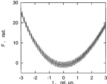
Fig. 2. Phase F(t) of the Green’s function G(t, L2) according to the stationary-phase method accounting for two stationary points (solid, jagged curve) and the third-order approximation of F(t) (dashed, smooth curve) used to evaluatew(t).
lationw (u) were determined by Eqs. (18)–(20) with the co-efficients fikobtained by approximating the phases of the Green’s functions G(u 2 t, L1) and G(t 2 u, L2)
com-puted accurately according to Eq. (5) (Fig. 2).
In practice, the accurate phase modulation required by Eqs. (18)–(20) can be introduced into the system when (a) the modulation running at some basic frequency vm is shifted in phase with respect to the main signal and (b) the second harmonic of the basic frequency vm is also used, so that the net modulation function is
w~u! 5 ~2w2/vm2!@1 2dcos~vmu 1 a! 2 g sin~2vmu!#, (23) where d5
A
11 «, tan(a) 5 «, « 5 (2/3vmw11 w3/vm)/ w2, and g 5 0.5(« 2 0.5vmw1/w2). For the case shownin Fig. 1, this means that, at the maximum modulation frequency vm5 0.1 consistent with the signal duration, the relevant parameters are « 5 0.32, d5 1.05, and g 5 0.16, so the phase shift of the modulation with respect to the signal is ;a 5 18° and the relative amplitude of the second harmonic is nearly 16%.
4. CONCLUSION
In conclusion, the results of this study have shown the possibility of increasing the accuracy of time imaging with an imperfect time lens by the proper choice of the phase-modulation function, depending on the dispersion law of the delay lines used in the lens.
ACKNOWLEDGMENTS
The author is grateful to K. A. Lukin for stimulating dis-cussions. The research was supported by the State Com-mittee on Science and Technology of Ukraine, project 2.3/ 827.
REFERENCES
1. B. H. Kolner and M. Nazarathy, ‘‘Temporal imaging with a time lens,’’ Opt. Lett. 14, 630–632 (1989).
2. B. H. Kolner, ‘‘Generalization of the concepts of focal length and f-number to space and time,’’ J. Opt. Soc. Am. A 11, 3229–3234 (1994).
3. B. H. Kolner, ‘‘Space–time duality and the theory of tempo-ral imaging,’’ IEEE J. Quantum Electron. 30, 1951–1953 (1994).
4. Ya. D. Shirman, Resolution and Compression of Signals (Soviet Radio, Moscow, 1974) (in Russian).
5. D. Grishkovskiy and A. C. Balant, ‘‘Optical pulse compres-sion based on enhanced frequency chirping,’’ Appl. Phys. Lett. 41, 1–3 (1982).
6. S. A. Akhmanov, V. A. Vysloukh, and A. S. Chirkin, ‘‘Self-action of wave packets in a nonlinear medium and fempto-second laser pulse generation,’’ Sov. Phys. Usp. 29, 642–677 (1987).
7. M. T. Kauffman, A. A. Godil, B. A. Auld, W. C. Banyai, and D. M. Bloom, ‘‘Applications of time lens optical systems,’’ Electron. Lett. 29, 268–269 (1993).
8. A. A. Godil, B. A. Auld, and D. M. Bloom, ‘‘Time-lens pro-ducing 1.9 ps optical pulses,’’ Appl. Phys. Lett. 62, 1047– 1049 (1993).
9. S. J. Farlow, Partial Differential Equations for Scientists and Engineers (Wiley, New York, 1982).
10. J. W. Goodman, Introduction to Fourier Optics (McGraw-Hill, New York, 1968).