Fractional correlation
David Mendlovic, Haldun M. Ozaktas, and Adolf W. Lohmann
Recently, optical interpretations of the fractional-Fourier-transform operator have been introduced. On the basis of this operator the fractional correlation operator is defined in two different ways that are both consistent with the definition of conventional correlation. Fractional correlation is not always a shift-invariant operation. This property leads to some new applications for fractional correlation as shift-variant image detection. A bulk-optics implementation of fractional correlation is suggested and demonstrated with computer simulations.
Key words: Fourier optics, optical information processing, fractional Fourier transforms, correlation.
1. Motivation
Correlation is a useful tool for pattern recognition comparison, or search. It is perhaps the most impor-tant special case of convolution. Correlation is easily implemented optically, for example, with the VanderLugt 4-f coherent configuration,1with its
analo-gous incoherent system,2or with the joint transform
correlator.3 The conventional correlation is a
shift-invariant operation; thus shifting of the input pattern provides a shifted correlation output plane. In other words, when an input object is viewed as a collection of point sources, each point source in the object generates the same point-spread function in the out-put image independent of the point-source location. The location of the point-spread function at the out-put plane corresponds to the location of the point source at the input plane. In many cases this prop-erty is necessary, but sometimes not. An example is when one wants to obtain a correlation peak only when a specific object appears at a certain location 1such as recognition of a stamp that could appear on a certain area of the envelope2. Another example is when one wants to base the recognition decision mainly on the central pixels and less on the outer pixels.
Several approaches for obtaining such space-variance detection have been suggested. One of
them used holographic filters that were made by use of reference beams with different angles.4 Another
approach was based on the use of different phase-encoded reference beams.5 Recently a space-variant
Fresnel-transform correlator was suggested.6 This
correlator is closely related to a lensless intensity correlator.7
In the following we suggest the use of the fractional Fourier transform 1FRT2 for implementing shift-variant pattern recognition. The FRT was defined mathematically by Namias.8 Some of his
mathemati-cal derivations were incomplete and were later im-proved by McBride and Kerr.9 Recently we
de-fined10–12the FRT operator based on physical1optical2
considerations. We discovered that our definition was equivalent to that given in Refs. 8 and 9. In these papers10–12 we also showed how to realize
optically the two-dimensional FRT as well as various mathematical and physical properties. Very re-cently, an alternative definition of the fractional Fou-rier transform was suggested13 and shown to be
equivalent to both previous definitions.14 In
retro-spect this later definition emphasizes one of the most important properties of the FRT: its elegant presen-tation at the Wigner-distribution plane.
In Ref. 10 a new direction for generalizing the conventional correlation operation is mentioned briefly. It is based on the fractional Fourier trans-form and is thus coined fractional correlation. Con-ventional in this context means the standard Fourier mathematics.15 In the following we extend the
frac-tional correlation and investigate its use for object detection. As we will see, there is more than one way to define the fractional correlation based on the conventional correlation. We use computer simula-tions to demonstrate some simple examples of the options of using the fractional correlation operator.
D. Mendlovic is with the Faculty of Engineering, Tel Aviv University, Tel Aviv 69978, Israel. H. M. Ozaktas is with the Department of Electrical Engineering, Bilkent University, Ankara 06533, Bilkent, Turkey. A. W. Lohmann is with the Angewandte Optik, Erlangen University, Erlangen 8520, Germany.
Received 2 November 1993; revised manuscript received 1 June 1994.
0003-6935@95@020303-07$06.00@0.
2. Notations and Definitions
2.A. Conventional Fourier Transform
Functions f and g are a Fourier pair if F1n2 5
e
2` ` f1x2exp12i2pnx2dx, 112 f1x2 5e
2` ` F1n2exp1i2pxn2dn. 122 In operator notation we may writeF1n2 5 F f 1x2. 132
It is well known that F2f1x2 5 f 12x2 and F4f1x2 5 f1x2, where Fj
i means application of F j times in
succession.
2.B. Fractional Fourier Transform
Reference 10 describes the original fractional-Fourier-transform definition, which is based on the Hermite– Gaussian functions 1the self modes of a quadratic graded-index medium2. For the following analysis the Wigner-distribution interpretation of the frac-tional Fourier transform is more convenient because its optical interpretation contains bulk-optics ele-ments that provide a high space–bandwidth product for comparing the graded-index elements. In fact, it was proposed as alternative definition of the frac-tional Fourier transform13 and later proved14 to be
equivalent to the Hermite–Gaussian function defini-tion. This definition states that performing the Pth fractional-Fourier-transform operation corresponds to rotating the Wigner-distribution by an angle
f 5 P1p@22 142
in the clockwise direction. Detailed discussion of the Wigner distribution may be found in Refs. 16–20. Figure 1 shows the suggested optical setup for per-forming a fractional Fourier transform of order P. It contains two lenses with the focal length f 5 f1@tan1f@22 with a space of z 5 f13sin1f24 between
them. f1is a free parameter. When P 5 1 and f 5
p@2, f 5 z 5 f1, which is related to the classical Fourier
transform. The effect of propagation of a signal through this setup is equivalent to performing an FRT of order P1 FP2 and can be expressed as
FP3u01x24 5 uP1x2 5
e
2` ` uo1x02exp3
ip1
x21 x 0 2 T24
3 exp1
2i2pxx0 S2
dx0, 152 with T 5 lf1tan1f2, S 5 lf1sin1f2, 162where l is the wavelength of the incident light.
2.C. Conventional Correlation
The conventional correlation of u01x2 and v01x2 is
defined as C11x2 5
e
2` ` u01x02v*01x 2 x2dx0 5e
2` ` u11n2v*11n2exp1i2pnx2dn, 172 where u11n2 5 F1u01x2, v11n2 5 F1n01x2. 182For what follows, the spectral definition of the correlation 3see Eq. 1724 includes the following: Perform the first Fourier transform of both objects, take the complex conjugate of one of the objects, multiply the results, and finally, perform an inverse Fourier transform.
3. Basic Properties Proposed for the Definition of Fractional Correlation
Three basic requirements from the fractional correla-tion CP1x2 are considered. The first one is mandatory:
if P 5 1, CP1x2 = C11x2. 192
In addition, we consider two weaker requirements whose satisfaction is not as critical as postulate 192. One is connected with the autocorrelation center value for every P:
if v 5 u, CP102 5 C1102 5
e
2``
0u01x0202dx0. 1102
Note that u, v should be located at the same location, and thus the conventional correlation C11x2
obtains its maximum at x 5 0 1while v 5 u2. This means that C1102 $ C11x2 for every x.
The third postulate ensures that P 5 0 means a
Fig. 1. Bulk-optics setup for performing a fractional Fourier transform of order P. f and z depend on P.
regular multiplication of u and v*:
if P 5 0, C01x2 5 u01x2v*01x2. 1112
In Section 4, two fractional correlation definitions that follow postulate192 are presented.
4. Various Fractional Correlation Definitions
Before defining the fractional correlation operation, we first show what the steps are for performing the conventional correlation. Two approaches can be used for obtaining the conventional correlation. The first approach is as follows:
112 Start with u01x02 and v01x02.
122 Perform F1 on both functions to obtain u 11 y2
and v11 y2.
132 Perform the complex conjugate of v11 y2.
142 Perform the multiplication u11 y2 v*11 y2 to
obtain F1C 1.
152 Perform F21to obtain C 11x2.
The second approach is as follows: 112 Start with u01x02 and v01x02.
122 Perform v01x02 = v*012x02.
132 Perform F1 on both functions to obtain u 11 y2
andv*11 y2.
142 Multiply u11 y2v*11 y2 to obtain F1C11x2.
152 Perform F21to obtain C 11x2.
It is a fact that both approaches lead to the same output C11x2. In both processes, by replacing the F1
and F21operators with those of fractional order FP1
and FP2, respectively, we can define the fractional
correlation operator in such a way as to fulfill manda-tory postulate 192. However, the two definitions are not necessarily identical for P1, P2fi 1. For example,
to check postulate 1112, we should replace all the Fourier-transform operations with F0, which is the
identity operator. Thus the first approach results in C01x2 5 u01x2v*01x2 and the second in C01x2 5 u01x2v*012x2.
The second result is different from postulate 1112. Of course, postulate 1112 can be modified to fit the second approach.
Now let us look at an interesting property of the FRT:
FPv*012x2 5 v*2P12x2 5 v*22P1x2. 1122
With this relation, steps 2 and 3 of the second approach can be replaced by the following step: Perform FPu
01x2 and 3 F22Pv01x24*.
5. Generic Form of the Fractional Correlation Output Now let us write explicitly the output signal CP1x2.
In order to investigate the most general case, we assume P 5 P1 for the fractional Fourier operators
before the multiplications1step 4 in both approaches2 and P 5 P2for the fractional Fourier transform after
the multiplications. It is not necessary that P15 P2,
and thus we denote the correlation output CP1,P2.
When Eq.152 is substituted instead of the F operator, CP1,P2becomes CP1,P21x2 5
e
2` `e
2``e
2`` u01x02v0 *16x˜ 02 3 exp3ipC11x, x0, x˜0, y243 exp32i2pC21x, x0, x˜0, y24dx0dx˜0dy, 1132
with C11x, x0, x˜0, y2 5 x21 y2 T2 1x0 21 y2 T1 7x˜0 21 y2 T1 , 1142 C21x, x0, x˜0, y2 5 y
1
x07 x˜0 S1 1 x S22
, 1152 T15 lf1tan1f12, T25 lf1tan1f22, 1162 S15 lf1sin1f12, S25 lf1sin1f22, 1172 f15 P11p@22, f25 P21p@22, 1182while f1 is a constant. Regarding the 6 and 7
symbols, the upper symbol is for the first approach, while the lower symbol is for the second approach. 6. Special Cases
6.A. Symmetric Case
We now want to reduce the triple integral of Eq.1132. The variable y is the only one that does not occur in the object functions u0 and v*0 of the integrand.
Hence, by using a well-known finite integral,21 the
saddle-point integration method e . . . dy can be esti-mated, and Eq.1132 becomes
CP1,P21x2 5
e
2` `e
2`` u01x02v*01x˜02 exp12ip@4210
1 T2 11 7 1 T102
1@2 3 exp5
ip3
1
x 2 T2 1x0 27 x˜ 0 2 T12
11
x07 x˜0 S1 1 x S22
2 1 T2 11 7 1 T146
3 dx0dx˜0. 1192Unfortunately, it is complicated to reduce the last general expression of CP1,P2to a single integral form as
in the conventional correlation expression 3see Eq. 1724. However, in Subsections 6.B and 6.C we present two special cases in which the final fractional correlation expression is a single integral.
Let us consider the symmetric case of P2 5 2P1.
Here
and thus for this case Eq.1192 is CP1,P21x2 5
e
2` `e
2`` u01x02v*01x˜02 exp12ip@42 101@T1021@2 3 exp5
ip31
2x 21 x 0 27 x˜ 0 2 T12
7 T11
x07 x˜02 x S12
246
dx0dx˜0. 1212Equation 1212 is shorter than Eq. 1192 but still contains two integrals. The above symmetric case should be considered as the most logical way for defining the fractional correlation operator because of its similarity to the conventional correlation. How-ever, the nonsymmetrical definitions that are dis-cussed in Subsections 6.B and 6.C lead to single integral expressions, which is certainly desirable.
6.B. Modified Case I
Let us now investigate the case in which e . . . dy is a Dirac integral. We can achieve this by choosing T1
and T2 such that no y2 occurs in the exponent.
Application of this condition to Eq.1142 when the first definition of fractional correlation is used yields
1@T25 0, 1222 or P25 1, S25 l f. 1232 On the basis of
e
2`` exp3
2i2py1
x02 x˜0 S1 1 x S224
dy 5 d1
x02 x˜01 S1 S2 x2
, 1242 one obtains CP1,11x2 5 exp3
2ip 1S1@S222 T1 x24
e
2` ` u01x02v*0 31
x01 S1 S2 x2
exp1
2i2p T1 S1 S2 xx02
dx0 1252as the final formula for fractional correlation. In this case we have S1@S2 5 sin1f12 and S1@1T1S22 5
cos3f1@1l f 24.
Another nice feature of this modification is that postulate1102 is fulfilled because
CP1,1102 5
e
2` ` u01x02u*01x02dx05e
2` ` 0u01x0202dx0. 1262For this case, postulate1112 is not fulfilled.
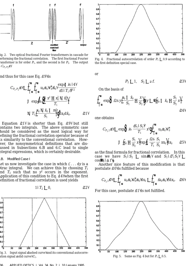
Fig. 2. Two optical fractional Fourier transformers in cascade for performing the fractional correlation. The first fractional Fourier transformer is for order P1, and the second is for P2. The output
is CP1,P21x2.
Fig. 3. Input signal1dashed curve2 and its conventional autocorre-lation signal1solid curve2 C1.
Fig. 4. Fractional autocorrelation of order P15 0.9 according to
the first definition special case.
6.C. Modified Case II
When the second definition of fractional correlation is applied, the y integral of Eq.1132 is a Dirac integral if
T25 2T1@2, 1272 and we obtain
e
2`` exp3
2i2py1
x01 x˜0 S1 1 x S224
dy 5 d1
x01 x˜01 S1 S2 x2
. 1282 The output is CP1,P21x2 5 exp3
2ip 1S1@S222 T1 x24
e
2` ` u01x02v*0 31
2x02 S1 S2 x2
exp1
2i2p T1 S1 S2 xx02
dx0. 1292Equation 1292 has a form similar to Eq. 1252. Although postulates 1102 and 1112 are not fulfilled now, they can be modified for this special case. Postulate 1102 may now be spelled out as the
follow-ing: if u 5 v, CP1,P2102 5 C11x2 5
e
2` ` u01x02u*012x02dx. 1302 Postulate1112 may now be written as the following:if P15 P25 0, C0,01x2 5 u01x2v*012x2. 1312
7. Optical Implementation
Figure 1 shows the optical setup for performing a fractional Fourier transform of order P. Following the definition of the fractional correlation, one can generate a modified matched filter
H11x2 5 5 FP1v1x26* 1322
for the first approach and
H21x2 5 FP1v*12x2 1332
for the second approach. This modified matched filter is placed between two optical fractional Fourier transformers, as shown in Fig. 2. The output is CP1,P2.
How can we generate the modified matched filter? There are two possibilities:
112 We can use computer-generated hologram
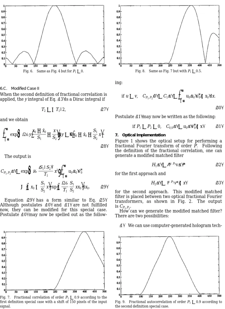
tech-Fig. 6. Same as Fig. 4 but for P15 0.
Fig. 7. Fractional correlation of order P15 0.9 according to the
first definition special case with a shift of 150 pixels of the input signal.
Fig. 8. Same as Fig. 7 but with P15 0.5.
Fig. 9. Fractional autocorrelation of order P15 0.9 according to
niques. Because in general the modified matched filter is a complex amplitude function, only phase and amplitude coding techniques are satisfactory, such as the detour phase method.22
122 We can use direct holographic means in a way similar to that suggested by VanderLugt1 for
record-ing the conventional matched filter. The reference object is placed at the input of the setup of Fig. 1, and the output is illuminated with a tilted plane wave as a reference beam. At the output a holographic plate is placed that, after exposure, is the matched filter. In both methods the fractional correlation signal CP1,P2is obtained along the first diffraction order.
8. Computer Simulations
In order to illustrate the use of fractional correlation, we performed computer simulations according to the optical setup of Fig. 2 using a MATLAB subroutine. The FRT was computed based on the Hermite– Gaussian modes FRT definition; we did not follow the Wigner FRT definition. This was done for the sake of shorting the computing time. We simulated only the two special cases that were introduced in Section 6. Simulations of the fractional Fourier transform itself can be found in Ref. 11. First, we simulated the conventional correlation. Figure 3 shows the input signal 1a rect function2 and its conventional autocorrelation. With the first definition, exactly the same result is obtained for P1 5 1. Now, let us
reduce P1. Figures 4, 5, and 6 are the fractional
autocorrelation following the first definition with orders P1equal to 0.9, 0.5, and 0, respectively1P25 1
for this case2. Figures 7 and 8 are the 0.9 and 0.5 fractional correlation output after shifting of one of the signals with 150 pixels. By inspection one can notice that for the P1 5 0.5 case the fractional
correlation is not shift invariant.
Similar simulations were performed for the second definition. Figure 31the conventional correlation2 is the fractional autocorrelation of order P15 1
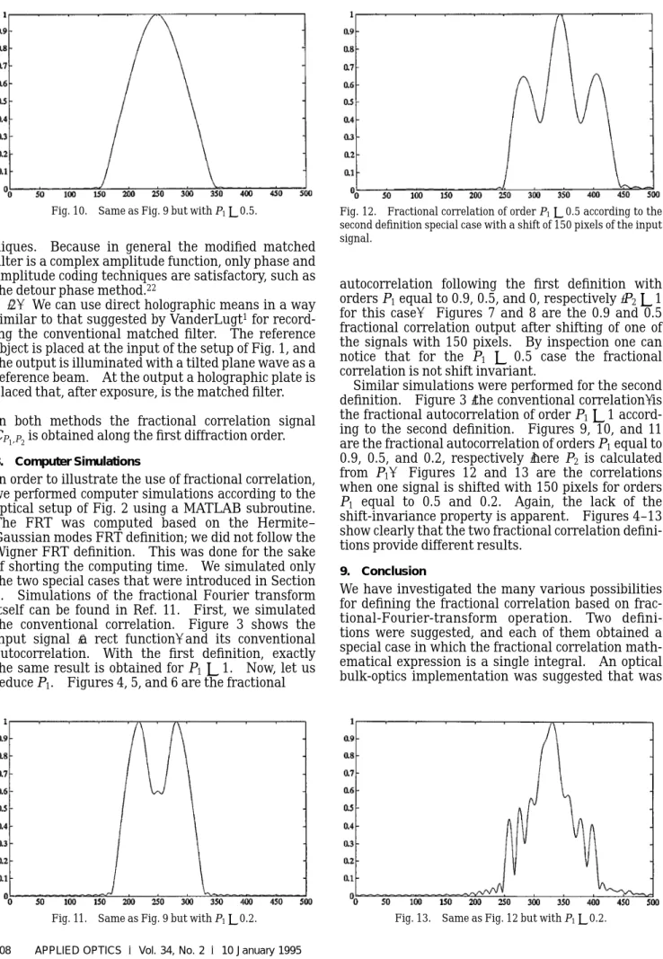
accord-ing to the second definition. Figures 9, 10, and 11 are the fractional autocorrelation of orders P1equal to
0.9, 0.5, and 0.2, respectively 1here P2 is calculated
from P12. Figures 12 and 13 are the correlations
when one signal is shifted with 150 pixels for orders P1 equal to 0.5 and 0.2. Again, the lack of the
shift-invariance property is apparent. Figures 4–13 show clearly that the two fractional correlation defini-tions provide different results.
9. Conclusion
We have investigated the many various possibilities for defining the fractional correlation based on frac-tional-Fourier-transform operation. Two defini-tions were suggested, and each of them obtained a special case in which the fractional correlation math-ematical expression is a single integral. An optical bulk-optics implementation was suggested that was
Fig. 10. Same as Fig. 9 but with P15 0.5.
Fig. 11. Same as Fig. 9 but with P15 0.2.
Fig. 12. Fractional correlation of order P15 0.5 according to the
second definition special case with a shift of 150 pixels of the input signal.
very similar to the conventional 4-f correlator. Computer simulations demonstrated that the frac-tional correlation operator is sometimes not a shift-invariant operator. In a similar way the fractional convolution can be defined as discussed in Ref. 23. In a future study the usefulness of this new operator for object detection will be checked according to important criteria such as signal-to-noise ratio, peak height, and light efficiency.
References
1. A. VanderLugt, ‘‘Signal detection by complex spatial filtering,’’ IEEE Trans. Inf. Theory IT-10, 139–146119642.
2. A. W. Lohmann and H. W. Werlich, ‘‘Incoherent matched filter with Fourier holograms,’’ Appl. Opt. 7, 561–563119682. 3. C. S. Weaver and J. W. Goodman, ‘‘A technique for optically
convolving two functions,’’ Appl. Opt. 5, 1248–1249119662. 4. L. M. Deen, J. F. Walkup, and M. O. Hagler, ‘‘Representations
of space-variant optical systems using volume holograms,’’ Appl. Opt. 14, 2438–2446119752.
5. T. F. Krile, R. J. Marks, J. F. Walkup, and M. O. Hagler, ‘‘Holographic representations of space-variant systems using phase-coded reference beams,’’Appl. Opt. 16, 3131–3135119772. 6. J. A. Davis, D. M. Cottrell, N. Nestorovic, and S. M. Highnote, ‘‘Space-variant Fresnel transform optical correlator,’’ Appl. Opt. 31, 6889–6893119922.
7. G. G. Mu, X. M. Wang, and Z. Q. Wang, ‘‘A new type of holographic encoding filter for correlation: a lensless inten-sity correlator,’’ in Holographic Applications, J. Ke and R. J. Pryputniewicz, eds. Proc. Soc. Photo-Opt. Instrum. Eng. 673, 546–549119862.
8. V. Namias, ‘‘The fractional Fourier transform and its applica-tion in quantum mechanics,’’ J. Inst. Math. Its Appl. 25, 241–265119802.
9. A. C. McBride and F. H. Kerr, ‘‘On Namias’s fractional Fourier transforms,’’ IMA J. Appl. Math. 39, 159–175119872.
10. D. Mendlovic and H. M. Ozaktas, ‘‘Fractional Fourier transfor-mations and their optical implementation: I,’’ J. Opt. Soc. Am. A 10, 1875–1881119932.
11. H. M. Ozaktas and D. Mendlovic, ‘‘Fractional Fourier transfor-mations and their optical implementation: II,’’ J. Opt. Soc. Am. A 10, 2522–2531119932.
12. H. M. Ozaktas and D. Mendlovic, ‘‘Fourier transform of fractional order and their optical interpretation,’’ Opt. Com-mun. 101, 163–169119932.
13. A. W. Lohmann, ‘‘Image rotation, Wigner rotation, and the fractional Fourier transform,’’ J. Opt. Soc. Am. A 10, 2181– 2186119932.
14. D. Mendlovic, H. M. Ozaktas, and A. W. Lohmann, ‘‘Graded-index fibers, Wigner distribution functions, and fractional Fourier transform,’’ Appl. Opt. 33, 6182–6187119942.
15. J. W. Goodman, Introduction to Fourier Optics1McGraw-Hill, New York, 19682, Chap. 7.
16. E. Wigner, ‘‘On the quantum correction for thermodynamic equilibrium,’’ Phys. Rev. 40, 749–759119322.
17. M. J. Bastiaans, ‘‘The Wigner distribution function applied to optical signals and systems,’’ Opt. Commun. 25, 26–30119782; ‘‘Wigner distribution function and its application to first-order optics,’’ J. Opt. Soc. Am. 69, 1710–1716119792.
18. H. O. Bartelt, K.-H. Brenner, and A. W. Lohmann, ‘‘The Wigner distribution function and its optical production,’’ Opt. Com-mun. 32, 32–38119802.
19. T. A. C. M. Claasen and W. F. G. Mecklenbraucker, ‘‘The Wigner distribution: a tool for time-frequency signal analysis: Part 1: Continuous time signals,’’ Philips J. Res. 35, 217–250 119802.
20. T. A. C. M. Claasen and W. F. G. Mecklenbraucker, ‘‘The Wigner distribution: a tool for time-frequency signal anslysis: Part 2: Discrete time signals,’’ Philips J. Res. 35, 276–300 119802.
21. M. Abramovitz and I. A. Stegun, Handbook of Mathematical Functions1Dover, New York, 19702.
22. A. W. Lohmann and D. P. Paris, ‘‘Binary Fraunhofer holograms generated by computer,’’ Appl. Opt. 6, 1739–1748119672. 23. H. M. Ozaktas, B. Barshan, D. Mendlovic, and L. Onural,
‘‘Convolution, filtering, and multiplexing in fractional Fourier domain and their relation to chirp and wavelet transform, J. Opt. Soc. Am. A 11, 547–559119942.