Observer based synchronization of chaotic systems

Observer based synchronization of chaotic systems

O¨ mer Morgu¨l*and Ercan Solak

Department of Electrical and Electronics Engineering, Bilkent University, 06533, Bilkent, Ankara, Turkey ~Received 22 April 1996; revised manuscript received 9 August 1996!

We show that the synchronization of chaotic systems can be achieved by using the observer design tech-niques which are widely used in the control of dynamical systems. We show that local synchronization is possible under relatively mild conditions and global synchronization is possible if the chaotic system can be transformed into a special form. We also give some examples including the Lorenz, the Ro¨ssler systems, and Chua’s oscillator which are known to exhibit chaotic behavior, and show that in these systems synchronization by using observers is possible.@S1063-651X~96!10511-0#

PACS number~s!: 05.45.1b

I. INTRODUCTION

The concept of synchronization of chaotic systems may seem somewhat paradoxical since in such systems solutions starting from arbitrary close initial conditions quickly di-verge and become uncorrelated. However, recently it has been shown that such synchronization is possible, see e.g.,

@1–3#, and this subject then received a great deal of attention

among scientists in many fields @1–9#. One of the motiva-tions for synchronization is the possibility of sending mes-sages through chaotic systems for secure communication

@4–6#. Such synchronized systems usually consist of two

parts: a generator of chaotic signals~drive system!, and a receiver~response system!. The response system is usually a duplicate of a part ~or the whole! of the drive system. A chaotic signal generated by the drive system may be used as an input in the response system to synchronize the common signals of both systems, see e.g.,@2#. After the synchroniza-tion, one may add the message to the chaotic signal used for synchronization, and under certain conditions one may re-cover the message from the signals of the response system

@4#. We note that once the chaotic ‘‘drive’’ system is given,

most of the synchronization schemes proposed in the litera-ture do not give a systematic procedure to determine the ‘‘response’’ system and the drive signal. Hence most of these schemes depend on the choice of the drive system and could not be easily generalized to an arbitrary chaotic drive system. A related problem encountered in the systems and control theory is the estimation of the states of a dynamical system by using another system, called an ‘‘observer.’’ The theory of the design of observers, although not fully exploited, is a relatively well-studied branch of system theory and is widely used in the state feedback control of dynamical systems@10– 16#. In this paper our aim is to show that this existing theory of observers may naturally be used in the relatively new field of synchronization of chaotic systems. In this approach, once the drive system is given, the response system could be cho-sen in the observer form, and the drive signal should be chosen accordingly so that the drive system satisfies certain conditions. Under some relatively mild conditions, local or

global synchronization of drive and observer systems can be guaranteed. Hence this synchronization scheme offers a sys-tematic procedure, independent of the choice of the drive system. It is our belief that the interaction between these fields may be beneficial for both of the fields.

This paper is organized as follows. In Sec. II we present some basic material for the design of observers and show that local synchronization may be possible under certain con-ditions, which are not very restrictive. We consider the Lo-renz and Ro¨ssler systems and show that for these systems local synchronization may be possible by using the observ-ers. We also show that some of the existing schemes for synchronization~e.g., @2,3#! are related to the observer based synchronization. We also show that the proposed synchroni-zation scheme is robust with respect to measurement noise. In Sec. III we consider a special form called the Brunowsky canonical form and by using the result of @12# show that if the chaotic system can be transformed into this form, global synchronization is possible. We also show that some of the chaotic systems ~e.g., the Ro¨ssler system and Chua’s oscil-lator! can be transformed into this form. In Sec. IV we present some numerical simulation results and finally, in Sec. V, we give some concluding remarks.

II. FULL ORDER OBSERVER

We begin with the definition of observability for a linear system, which plays an important role in modern control theory. Consider the following linear system:

u˙5Au, y5Cu, ~1!

where APRn3n, CPRm3n are constant matrices, y is called the ‘‘output’’ of the system. The problem of observability is related to the computation of initial condition u~0!PRn by only observing the output y~•! over an interval of time.

Definition:~Observability! Consider the system described by~1!. Two states u0and u1are said to be distinguishable if

y (t,u0)Þy(t,u1) for some t>0, where y(t,ui)5CeAtui, is the output y (t) corresponding to the initial condition u(0)5u_i, i51,2. The system given by ~1! @or, in short, the pair (C,A)# is said to be observable if all distinct states are distinguishable~see, e.g., @14,13,15#!.

We next state the following well-known fact. *Fax: 90-312-266 41 26;

Electronic address: morgul@bilkent.edu.tr

54

Theorem 1: Consider the system given by ~1!. Then the following are equivalent:

~i! The pair (C,A) is observable.

~ii! The following rank condition is satisfied:

rank

S

C CA • • • CAn21

D

5n. ~2!

~iii! The following rank condition is satisfied:

rank

S

lI2A

C

D

5n, ;lPC. ~3!

~iv! For any polynomial p(l)5ln_1a

1l

n_{211• • •1} an₂₁l1an, aiPR, i51,2, . . . ,n, there exists a constant matrix KPRn3m such that det(lI2A1KC)5p(l).

Proof: See e.g.,@13#, p. 80, p. 136, and @15#, p. 61. Consider the nonlinear system given below

u˙5Au1g~u!, y5Cu, ~4!

where APRn3n and CPRm3n are constant matrices, g:

Rn→Rn is a differentiable function. Assume that g satisfies the following Lipschitz condition:

ig~u1!2g~u2!i<Liu12u2i, ;u1,u2PRn, ~5!

where L.0 is a Lipschitz constant and i•i is the standard Euclidean norm inRn. We will use a technique proposed in

@10# for the observer design. We assume that the pair (C,A)

is observable. Now choose the matrix KPRn3m such that A_c5A2KC is a stable matrix, which is always possible since the pair (C,A) is observable, see Theorem 1. Then for any symmetric and positive definite matrix QPRn3n there exists a symmetric and positive definite matrix PPRn3n such that the following well-known Lyapunov matrix equa-tion is satisfied:

A_cTP1PAc52Q, ~6!

where the superscript T denotes the transpose @14#. For the system given by ~4!, we choose the following ‘‘observer’’ equation:

uˆ

˙ 5Auˆ1g~uˆ!1KC~u2uˆ!, ~7!

which is known as the full order observer or the Luenberger observer@12#. Note that the signals y5Cu and uˆ are avail-able, hence, the observer given by~7! is implementable. Let us define the error of observation as e5u2uˆ. By using ~4! and~7! we obtain the following error equation:

e˙5~A2KC!e1g~u!2g~uˆ!. ~8!

Now let the symmetric and positive definite matrices P and Q satisfy ~6!. By using the Lyapunov function V5eTPe, it can be shown that if

L, lmin~Q! 2lmax~P!

, ~9!

then we have the following:

ie~t!i<Me2atie~0!i, ~10!

where M5

F

lmax~P! lmin~P!

G

1/2 , a5 lmin~Q! 2lmax~P! 2L.0,

and l_max(T), l_min(T) denote the maximum and minimum eigenvalues of a symmetric matrix T, respectively. For de-tails, see@10#, and for a survey on observer theory, see @11#. In the application of the observer theory given above, the main difficulty is in the Lipschitz property given by ~5!, which should be satisfied globally. But if~5! is satisfied, then the observer given by ~7! works globally, i.e., for all e~0!PRn, provided that ~9! is satisfied. We may relax this condition as follows, but then the result ~10! may hold lo-cally, i.e., in a compact region for e~0!.

Lemma 1: Consider the systems given by ~4! and ~7!. Assume that the pair (C,A) is observable, g:Rn→Rn is dif-ferentiable and that the following is satisfied:

lim u_→0

iDg~u!i50, ~11!

where Dg~•! denotes the Jacobian of g. Then there exist a matrix KPRn3mand a real number r.0 such that ~10! holds if ie(0)i<r and iu(t)i<r, ;t>0.

Proof: Choose a matrix KPRn3m such that Ac5A2KC is a stable matrix, and choose the symmetric and positive definite matrices P and Q which satisfy ~6!. For R.0, we may take L.0 in ~5! as

L5sup$iDg~u!iuiui<R%. ~12! Now choose R.0 such that L.0 given by ~12! satisfies ~9!. Note that since ~11! holds, this is always possible. Let

iuˆ(0)i<r1andiu(t)i<r2,;t>0 for some r1.0 and r2.0.

By using the Bellman-Gronwall inequality, ~5! and ~7! ~see e.g.,@14,16#, it can be proven that if r1and r2are sufficiently

small, then uˆ(t) remains bounded as iuˆ(t)i<r3 for some

r₃.0. Moreover, as r₁→0 and r₂→0, we have r₃→0 as well. Hence there exists a r.0 satisfying R.r such that if

iu(t)i<r and ie(0)i<r, then we have iuˆ(t)i<R, hence the

Lipschitz constant L given by ~12! remains valid ;t>0. Then it follows that ~10! remains valid ;t>0.

Remark 1: Lemma 1 states that if~11! holds, if the initial error e~0! is sufficiently small and if u(t) remains in a suf-ficiently small region, then for the observer given by~7!, the estimate given by~10! is satisfied. Since in chaotic systems the solutions which are of interest to us are bounded, this lemma might be used for local synchronization. However, the lemma does not provide an estimate on the bound r. Note that the condition given by ~11! is less stringent than the Lipschitz condition~5! and ~9!. In applications, the differen-tial equation given by ~4! is obtained by linearization of a nonlinear system around an equilibrium point. In such cases, the function g necessarily contains at least second order terms, hence~11! is automatically satisfied.

The observer design technique given above assumes that an output y~•! which is transmitted to the observer is avail-able, see ~4! and ~7!. However, in chaotic systems such an output is not given a priori and has to be chosen as a part of the observer design procedure. In view of the observer theory given above, obviously one should choose the output as in

~4! so that the pair (C,A) is observable. ~The observability

condition may be changed to a ‘‘detectability’’ condition, which is weaker than observability. See Remark 3 and the Example 1 below!. Moreover, for practical considerations, the dimension m should be as low as possible, since y (t)PRmis the signal transmitted to the observer. Case m51 is possible under certain conditions, which are given below. Note that a matrix APRn3n is called cyclic if in its Jordan canonical form, for each eigenvalue of A there exists one and only one Jordan block. This guarantees that rank(liI2A)5n21 for any eigenvalue liof A.

Lemma 2: Let APRn3nbe given. Then there exists a vec-tor CTPRn such that (C,A) is observable if and only if A is cyclic.

Proof: This could easily be proven by using ~3!. More-over, letl1, . . . ,lpbe the eigenvalues andv1, . . . ,vpbe the corresponding eigenvectors of A. Then for any vector CTPRn which satisfies CviÞ0. i51,2, . . . ,p, the pair (C,A) is observable@13#.

Remark 2: The requirement that APRn3n be cyclic may seem a stringent condition. This condition is satisfied if all eigenvalues of A are distinct, and in the examples given be-low this condition is satisfied. Moreover, in most chaotic systems, the equations depend on certain parameters, and chaotic behavior is observed when these parameters are in certain ranges. In most cases the eigenvalues depend con-tinuously on these parameters; hence one may choose these parameters accordingly so that the system exhibits chaotic behavior and the matrix A has distinct eigenvalues. Then, by using Lemma 2, one may find a vector CTPRn so that the pair (C,A) is observable.

Remark 3: For a given pair (C,A), whether the observer given by~7! satisfies ~10! and Lemma 2 depends on whether the matrix Ac5A2KC is stable or not. For observable pairs, by Theorem 1 there always exists a matrix K such that Acis stable. For some pairs (C,A) there may exist a matrix K such that A_cis stable, even if the pair is not observable. Such pairs are called ‘‘detectable,’’ and for such pairs the observer given by ~7! could still be used @15#.

Example 1: ~Lorenz system! Consider the Lorenz system given below

x˙15s~x22x1!,

x˙252x1x31rx12x2, ~13!

x˙35x1x22bx3.

The parameters s.0, r.0 and b.0 are chosen so that the system exhibits chaotic behavior@2#.

We may write ~13! in the form given by ~4! where u5(x₁ x₂ x₃)T, A5

S

2s r 0 s 21 0 0 0 2b

D

, g~u!5

S

0 2x1x3 x1x2

D

. ~14! It follows easily that the selection of y5c₁x₁1c₂x₃ @i.e., C5(c₁ 0 c₂)#, or y5c₁x₂1c₂x₃ @i.e., C5(0 c₁ c₂)# yields the pair (C,A) observable for almost all values of c1

and c2, provided that uc1uÞ0, uc2uÞ0. For actual values, ~2!

should be checked. For C5(c₁ c₂ 0) the pair (C,A) is not observable but detectable, i.e., one can easily find matrices of the form K5(k1 k2 0)

T

such that A2KC is stable. In par-ticular, the selection of y5x1 @i.e., C5~1 0 0!#, or y5x2,

@i.e., C5~0 1 0!# makes the pair (C,A) detectable, hence by

an appropriate choice of K, one may obtain a stable matrix A2KC and use the observer given by ~7! for synchroniza-tion of chaos.

At this point we compare the observer given by~7! with some synchronization schemes proposed in@2# and @3#. Con-sider the following system:

xˆ˙15s~xˆ22xˆ1!, ~15!

xˆ˙252x1xˆ31rx12xˆ2, ~16!

xˆ˙35x1xˆ22bxˆ3. ~17!

In @2#, ~16! and ~17! are called the response system and in

@3#, ~15!–~17! are called the response system, for the drive

system given by~13!. Note that here x1 is used as the drive

signal, hence according to our observer design technique, the output of~13! is y5x₁. By using the Lyapunov theory, it can be shown that limt→`iu(t)2uˆ(t)i50, where u5(x1 x2 x3)

T

and uˆ5(xˆ1 xˆ2 xˆ3)

T

, see @2,3#. Note that

~15!–~17! could be written in the form

uˆ

˙ 5Auˆ1g~uˆ!1KC~u2uˆ!1F~uˆ!C~u2uˆ!, ~18!

where A and g are given in~14!, K5(0 r 0)T, C5~1 0 0! and F(uˆ)5(02xˆ3 xˆ2)T. Note that A2KC is a stable matrix

with this choice. Hence, the response system given by~15!–

~17!, and hence ~18!, is similar to the observer given by ~7!

except for the last term in~18!. Without this term Lemma 1 guarantees the local convergence of the error. However, due to the special structure of this term, now we can prove global

~exponential! convergence of the error. Due to the special

structure of this term, the error equation now becomes

e˙5~A2KC!e1S~t!e, ~19! where Ac5A2KC5

S

2s 0 0 s 21 0 0 0 2b

D

, S~t!5

S

0 0 0 0 0 x₁~t! 0 2x1~t! 0

D

. ~20!

Note that A_cis a stable matrix, hence the Lyapunov equation

particu-lar, P5diag~g,b,b! is a solution, provided that g.0, b.0 and 4b.gs, where diag denotes a diagonal matrix with the specified entries at its diagonal. Note that with this choice, we have PS(t)5S(t)P. Hence, by using Lyapunov function V5eTPe, differentiating along the error equation ~19!, we obtain V˙ 52eTQe, where Q is given by~6!. Therefore ~10! is valid for all e~0!PR3, where

a5 lmin~Q!

2lmax~P!

.

For the synchronization of Lorenz system, the following response system has also been proposed by@2,3,7#:

xˆ˙15s~x22xˆ1!,

xˆ˙252xˆ1xˆ31rxˆ12xˆ2, ~21!

xˆ˙35xˆ1x22bxˆ3.

Note that here x₂is used as the drive signal, hence according to our observer design technique, the output of~13! is y5x2.

It could be shown that for this response system, synchroni-zation is achieved. Note that ~21! could be written in the form of ~18!, where A and g are as given by ~14!, K5(s 0 0)T, C5~0 1 0!, and F(uˆ)5(0 0 xˆ₁)T. Hence, the response system given by ~21! and hence ~18!, is similar to the observer given by ~7! except for the last term in ~18!. Without this term, Lemma 1 may guarantee the local conver-gence of the error. With this term, the Lemma 1 is still valid ifuxˆ₁(t)u<M₁for some M₁.0, provided that in ~9!, the left hand side is replaced by L1M1. However, due to the form

of F~•!, we can show that ~10! is satisfied for some M.0 anda.0 provided that the solutions of ~13! are bounded. To see that, define e5(e₁ e₂ e₃)T. Then, from~18! it follows that e1(t)5e2ste1(0), and by using this first in the equation

for e3, and then in the equation for e2, we obtain exponential

decay for all error components, provided that x1(t), x2(t),

and x₃(t) are bounded. Since the Lorenz system exhibits chaotic behavior for the selected set of parameters, its solu-tions which are of interest to us are bounded; hence this condition is satisfied.

Example 2:~Ro¨ssler system! Consider the Ro¨ssler system given below:

x˙15x21ax1,

x˙252x12x3,

x˙35b2cx31x2x3, ~22!

where the parameters a.0, b.0 and c.0 are chosen so that the system exhibits chaotic motion, see@2#. This system may be written in the form given by ~4! where u5(x1 x2 x3) T , A5

S

a 21 0 1 0 0 0 21 2c

D

, g~u!5

S

0 0 b1x2x3

D

. ~23! It can easily be shown that the selection of y5c₁x₁1c₂x₂1c₃x₃ @i.e., C5(c₁ c₂ c₃)# yields the pair

(C,A) observable for almost all c₁, c₂, and c₃, provided that

uc1u1uc2uÞ0. For actual values, ~2! should be checked. In

particular, with the selection of y5x1 or y5x2, the

corre-sponding pairs (C,A) are observable; hence by choosing the feedback matrix K appropriately, the observer given by ~7! may achieve local synchronization. Note that with the selec-tion of y5x3, the corresponding pair (C,A) is not even

de-tectable; hence the observer given by ~7! could not be used for synchronization for this output.

In the rest of this section we show that the observer given by ~7! is robust with respect to measurement noise, i.e., the synchronization error remains bounded for bounded noise. To show this, we assume that the measured output y , which is used for synchronization in the observer, is corrupted with noise n(t), hence in~4! we have y5Cu1n. Then the error equation~8! becomes

e˙5Ace1g~u!2g~uˆ!2Kn~t!, ~24!

where A_c5A2KC is a stable matrix. We assume that the noise n(t) is bounded by some n_M.0, i.e., in(t)i<n_M,

;t>0, but arbitrary otherwise. Then the solution of ~24! can

be written as: e~t!5eAct_e~0!1

E

0 t eAc~t2t!$_g@u~t!#2g@uˆ~t!#%_dt 2

E

0 t eAc~t2t!_Kn~t!dt_. ~25! Since Ac is a stable matrix, it follows that the following is satisfied for some M.0 andd.0:

ieA_ct_i<Me2dt_{. ~26!} By using~26! and ~5! in ~25! and after some simple integra-tion and multiplicaintegra-tion by edt we obtain:

iedt_{e~t!i<Mie~0!i1}MiKinM d ~edt21! 1

E

0 t M Liedte~t!idt. ~27! Now by using a generalized form of the Bellman-Gronwall inequality, see e.g.,@16, p. 476# and after some simple inte-gration and algebra we obtain:

ie~t!i<A1nM1A2e2d

t_1A

3e2~d2ML!t, ~28!

for some constants A1, A2, and A3, where, in particular, we

have

A15

MiKi~d2ML11!

d~d2ML! .

Now let us assume that the Lipschitz constant L is suffi-ciently small so that d2ML.0, @cf. ~9!#. Then it follows from ~28! that the synchronization error is also bounded, which implies the stability of the proposed synchronization scheme in the presence of measurement noise. Moreover, asymptotically we haveie(t)i<A1nM. Since A1is

smaller the synchronization error and in the limit n_M→0, the synchronization error also asymptotically decays to zero. Hence, we may state that the proposed synchronization scheme is also efficient in this sense in the presence of noise. On the other hand, if the Lipschitz constant L is not suffi-ciently small but ~11! holds, then a similar result holds lo-cally; i.e., if ie(0)i and iu(t)i are sufficiently small, cf. Lemma 1. The proof of this fact is similar to that of Lemma 1 and is omitted here.

III. BRUNOWSKY CANONICAL FORM

In some cases, the local convergence result of the Lemma 1 could be extended to global convergence result, provided that the chaotic system given by ~4! has a special form. As-sume that the system is in the form~4! with

A5

S

0 1 0 ••• 0 0 0 1 ••• 0 . . . 0 0 0 ••• 1 0 0 0 ••• 0

D

, g~u!5

S

0 . . . 0 1

D

f~u!, C5~1 0 ••• 0!, ~29!

where f :Rn→R is a differentiable function and that g

satis-fies the Lipschitz property given by ~5!. The form given by

~29! is called the Brunowsky canonical form, and is

fre-quently used in the control of nonlinear systems @12,14#. Since the pair (C,A) is observable and g is Lipschitz, the observer given by~7! could be used for local convergence of error, provided that~9! is satisfied. However, it was shown in

@12# that for any L.0, one can find a feedback matrix K,

such that ~10! is satisfied when the system is in Brunowsky canonical form. Obviously this result still works if the sys-tem can be transformed into Brunowsky canonical form by means of a diffeomorphic coordinate transformation. The de-tails can be found in@12#. Here we give a procedure to select the desired K, different than the one considered in@12#.

For the design of the observer, choose l₁,0 and

l25gl1,l35g 2_l

1, . . . ,ln5g n21_l

1, where g.1. Consider

the following Vandermonde matrix:

V5

S

l1 n21 l2 n21 . . . ln n₂₁ l1 n22 l2 n22 ln n₂₂ ••• ••• ••• 1 1 1

D

. ~30!

It can easily be shown that the feedback matrix K5(k₁ k₂ . . . k_n)Tcan be appropriately chosen so that

Ac5A2KC5V21LV, ~31!

is satisfied, where L5diag ~l1,l2, . . . ,ln!. Now consider the error equation given by~8!, whose solution can be writ-ten as follows: e~t!5V21eLtVe~0!1V21 3

E

0 t eL~t2t!VB$f@u~t!#2 f @uˆ~t!#%dt, ~32! where B5(0 0 . . . . 1)T and eLt5diag~el1t_,el2t_{, . . . , e}lnt!,

By taking the max norm i•i_`~see e.g., @14#!, we obtain

ie~t!i`<iV21i`iVi`el1tie~0!i

` 1iV21<sub>i</sub> `

E

0 t el1~t2t!_Lie~t!i `dt, ~33! where we now assumed that ~5! is satisfied with the max norm. Note that since in Rn _{all norms are equivalent, this} only affects the Lipschitz constant L.0. Also, in ~33!, we used the matrix norm induced by the max norm. By multi-plying both sides of ~33! by e2l1t_{, using the}

Bellman-Gronwall Lemma, see e.g., @14#, we obtain

ie~t!i_`<iV21_i

`iVi`e~l11LiV21i`!tie~0!i`. ~34! Now simple calculation shows thatiV21i_`5G(g) for some rational function G~•!, provided that g and ul1u are

suffi-ciently large. Obviously once g.1 is chosen sufficiently large, then for anya.0 and L.0, one can choose l1so that

l11LiV21i`<2a. Hence, ~10! is satisfied with

M5iV21i_{`</sub>iVi<sub>`}andagiven by the inequality stated above. Note that some chaotic systems are already in the form given by ~4! and ~29! @17,18#; hence, the theory presented above can be directly applied for such systems. Some sys-tems may be transformed into this form by a coordinate transformation z5T(u), where T:Rn→Rn is a diffeomor-phism. The details of finding such a transformation may be found in@12#. Here we emphasize that for some systems this transformation may be linear, i.e., T(u)5Tu for some in-vertible matrix TPRn3n, hence the required transformation is quite simple. Now assume that the matrix A given in~4! is in the following form:

A5

S

* * * * a1 * * * 0 a2 * * 0 0 . . . * * ••• ••• ••• ••• 0 0 an21 *

D

, ~35!

where the entries given by the asterisk are arbitrary, and

aiÞ0 for i51,2, . . . ,n21. We also assume that g has the form given in ~29!. Under these conditions there exists a

linear and invertible transformation TPRn3n such that after the transformation z5Tu, in the transformed variables the system is given in the form~4! and ~29!. We note that in this case the required transformation has the form:

T5

S

1 0 0 0 ••• 0 * a1 0 0 ••• 0 * * a1a2 0 ••• 0 A * * * * a1a2•••an21

D

, ~36!

hence is always invertible.

Example 2:~revisited! Consider the Ro¨ssler system given by ~22!. Note that A given by ~23! is in the form given by

~35!. By choosing the transformation

z₁5x₁, z₂5ax₁1x₂, z₃5~a2_21!x

11ax22x3,

the Ro¨ssler system can be transformed into the form given by~4! and ~29!, where

f~z!52cz11~ca21!z21~a2c!z32az1 2_2az

2 2

1~a2_21!z

1z22az1z31z2z32b.

Since the function f given above is differentiable, it follows that the Lipschitz condition ~5! is satisfied in any compact region. Since the Ro¨ssler system exhibits chaotic behavior for certain values of the parameters a, b, and c, these chaotic solutions are bounded by a compact region, and in this re-gion~5! is satisfied for some L.0. An estimate of L can be found by usingiD f (z)i, see Lemma 1. Hence by using the technique presented above, an observer for which the syn-chronization error satisfies ~10! can be designed.

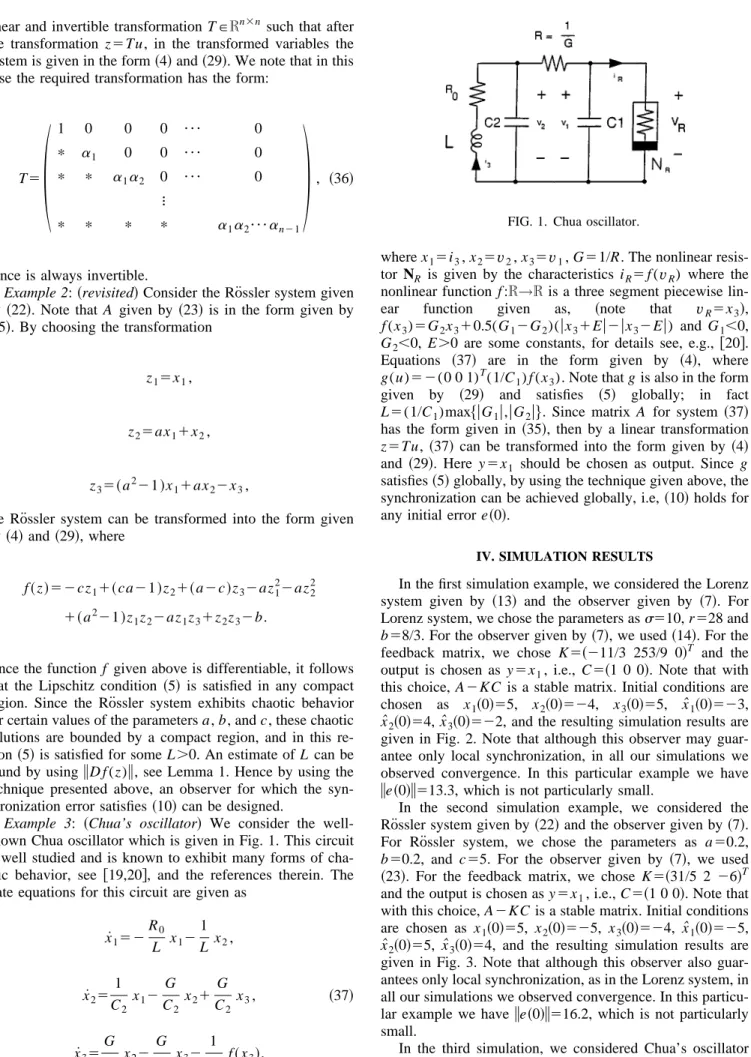
Example 3: ~Chua’s oscillator! We consider the well-known Chua oscillator which is given in Fig. 1. This circuit is well studied and is known to exhibit many forms of cha-otic behavior, see @19,20#, and the references therein. The state equations for this circuit are given as

x˙152 R0 L x12 1 L x2, x˙25 1 C2 x12 G C2 x21 G C2 x3, ~37! x˙35 G C1 x22 G C1 x32 1 C1 f~x3!,

where x15i3, x25v2, x35v1, G51/R. The nonlinear

resis-tor N_R is given by the characteristics i_R5 f (v_R) where the nonlinear function f :R→R is a three segment piecewise lin-ear function given as, ~note that vR5x3!,

f (x3)5G2x310.5(G12G2)(ux31Eu2ux32Eu) and G1,0,

G2,0, E.0 are some constants, for details see, e.g., @20#.

Equations ~37! are in the form given by ~4!, where g(u)52(0 0 1)T(1/C₁) f (x₃). Note that g is also in the form given by ~29! and satisfies ~5! globally; in fact L5(1/C1)max$uG1u,uG2u%. Since matrix A for system ~37!

has the form given in ~35!, then by a linear transformation z5Tu, ~37! can be transformed into the form given by ~4! and ~29!. Here y5x1 should be chosen as output. Since g

satisfies~5! globally, by using the technique given above, the synchronization can be achieved globally, i.e,~10! holds for any initial error e~0!.

IV. SIMULATION RESULTS

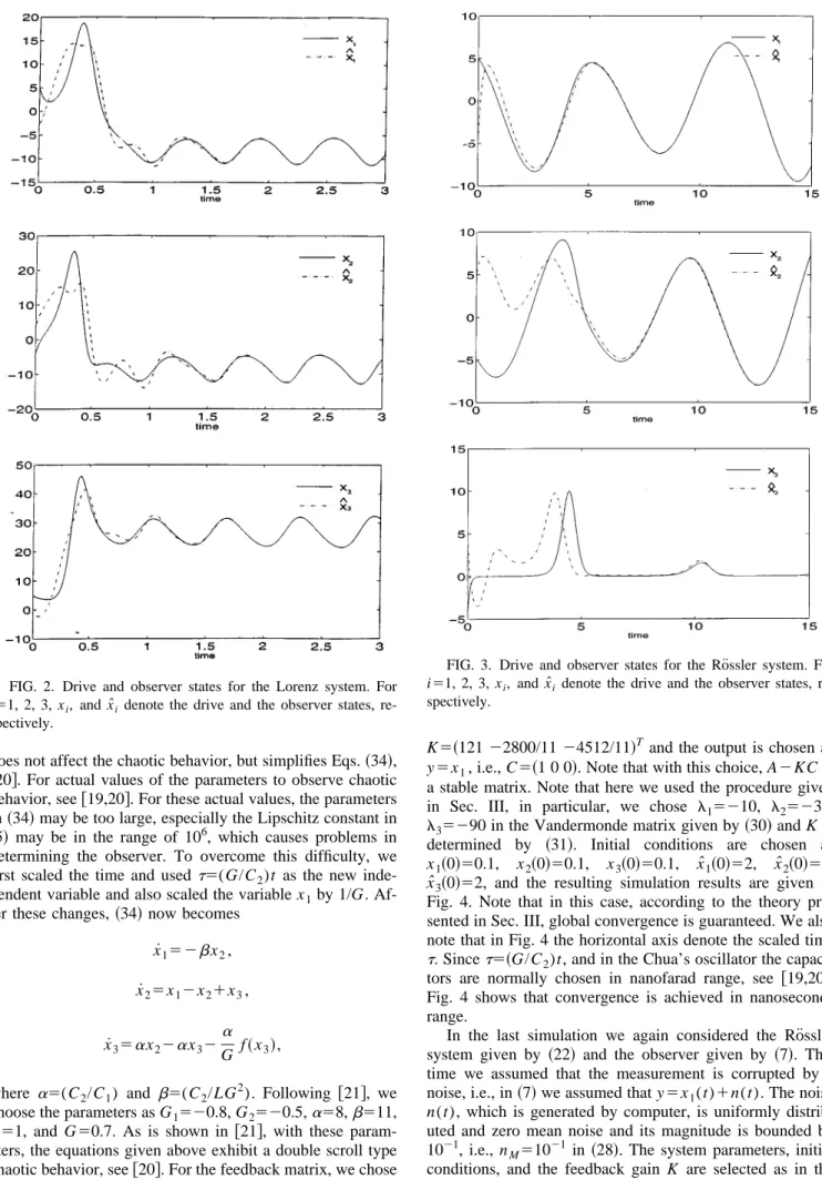
In the first simulation example, we considered the Lorenz system given by ~13! and the observer given by ~7!. For Lorenz system, we chose the parameters ass510, r528 and b58/3. For the observer given by ~7!, we used ~14!. For the feedback matrix, we chose K5~211/3 253/9 0!T and the output is chosen as y5x₁, i.e., C5~1 0 0!. Note that with this choice, A2KC is a stable matrix. Initial conditions are chosen as x1~0!55, x2~0!524, x3~0!55, xˆ1~0!523,

xˆ2~0!54, xˆ3~0!522, and the resulting simulation results are

given in Fig. 2. Note that although this observer may guar-antee only local synchronization, in all our simulations we observed convergence. In this particular example we have

ie~0!i513.3, which is not particularly small.

In the second simulation example, we considered the Ro¨ssler system given by~22! and the observer given by ~7!. For Ro¨ssler system, we chose the parameters as a50.2, b50.2, and c55. For the observer given by ~7!, we used

~23!. For the feedback matrix, we chose K5~31/5 2 26!T and the output is chosen as y5x1, i.e., C5~1 0 0!. Note that

with this choice, A2KC is a stable matrix. Initial conditions are chosen as x₁~0!55, x₂~0!525, x₃~0!524, xˆ₁~0!525, xˆ₂~0!55, xˆ₃~0!54, and the resulting simulation results are given in Fig. 3. Note that although this observer also guar-antees only local synchronization, as in the Lorenz system, in all our simulations we observed convergence. In this particu-lar example we have ie~0!i516.2, which is not particularly small.

In the third simulation, we considered Chua’s oscillator given in Fig. 1. In the simulations we chose R050, which

does not affect the chaotic behavior, but simplifies Eqs.~34!,

@20#. For actual values of the parameters to observe chaotic

behavior, see@19,20#. For these actual values, the parameters in~34! may be too large, especially the Lipschitz constant in

~5! may be in the range of 106_{, which causes problems in}

determining the observer. To overcome this difficulty, we first scaled the time and used t5(G/C₂)t as the new inde-pendent variable and also scaled the variable x₁by 1/G. Af-ter these changes, ~34! now becomes

x˙152bx2, x˙25x12x21x3, x˙35ax22ax32 a G f~x3!, where a5(C2/C1) and b5(C2/LG 2 ). Following @21#, we choose the parameters as G1520.8, G2520.5,a58,b511,

E51, and G50.7. As is shown in @21#, with these param-eters, the equations given above exhibit a double scroll type chaotic behavior, see@20#. For the feedback matrix, we chose

K5~121 22800/11 24512/11!Tand the output is chosen as y5x1, i.e., C5~1 0 0!. Note that with this choice, A2KC is

a stable matrix. Note that here we used the procedure given in Sec. III, in particular, we chose l₁5210, l₂5230,

l35290 in the Vandermonde matrix given by ~30! and K is

determined by ~31!. Initial conditions are chosen as x1~0!50.1, x2~0!50.1, x3~0!50.1, xˆ1~0!52, xˆ2~0!52,

xˆ3~0!52, and the resulting simulation results are given in

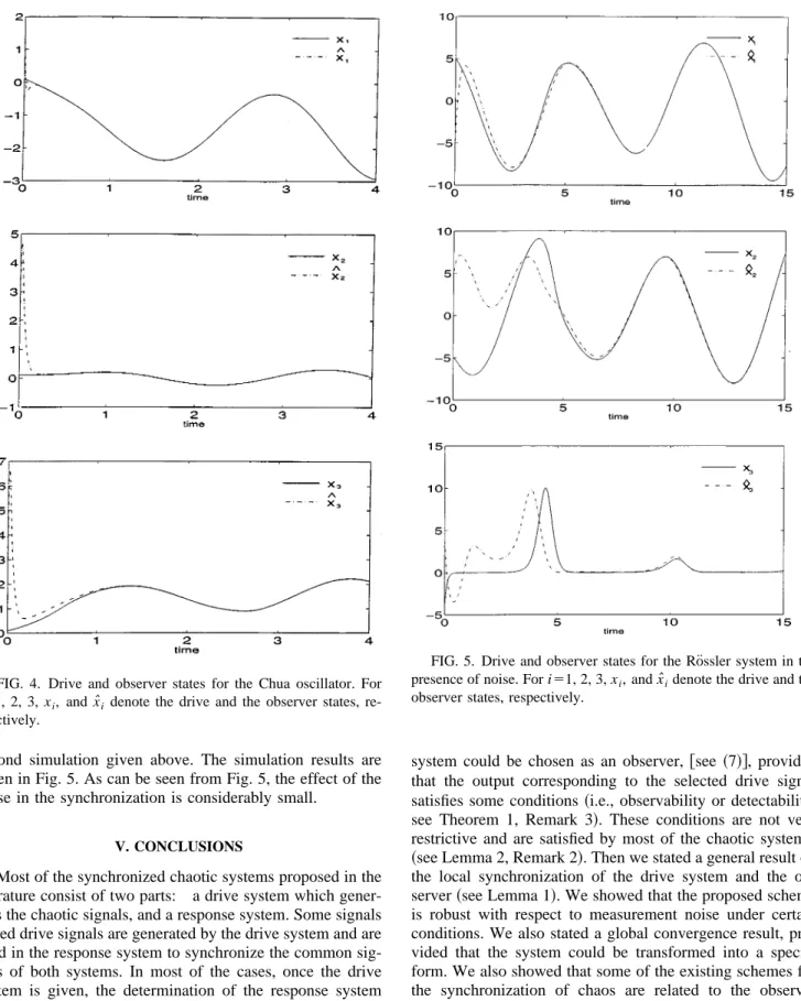
Fig. 4. Note that in this case, according to the theory pre-sented in Sec. III, global convergence is guaranteed. We also note that in Fig. 4 the horizontal axis denote the scaled time

t. Sincet5~G/C2)t, and in the Chua’s oscillator the

capaci-tors are normally chosen in nanofarad range, see @19,20#; Fig. 4 shows that convergence is achieved in nanoseconds range.

In the last simulation we again considered the Ro¨ssler system given by ~22! and the observer given by ~7!. This time we assumed that the measurement is corrupted by a noise, i.e., in~7! we assumed that y5x₁(t)1n(t). The noise n(t), which is generated by computer, is uniformly distrib-uted and zero mean noise and its magnitude is bounded by 1021, i.e., nM51021 in~28!. The system parameters, initial conditions, and the feedback gain K are selected as in the

FIG. 2. Drive and observer states for the Lorenz system. For

i51, 2, 3, xi, and xˆidenote the drive and the observer states,

re-spectively.

FIG. 3. Drive and observer states for the Ro¨ssler system. For

i51, 2, 3, xi, and xˆidenote the drive and the observer states,

second simulation given above. The simulation results are given in Fig. 5. As can be seen from Fig. 5, the effect of the noise in the synchronization is considerably small.

V. CONCLUSIONS

Most of the synchronized chaotic systems proposed in the literature consist of two parts: a drive system which gener-ates the chaotic signals, and a response system. Some signals called drive signals are generated by the drive system and are used in the response system to synchronize the common sig-nals of both systems. In most of the cases, once the drive system is given, the determination of the response system and the drive signals are not systematic and one scheme pro-posed for a particular drive system could not be easily gen-eralized to an arbitrary chaotic drive system.

In this paper we considered the observer based synchro-nization of chaotic systems. Observers are widely used in systems and control theory to estimate the states of a given system; hence they may naturally be used in the synchroni-zation of chaotic systems. In this approach, once the chaotic drive system is given in a form @see ~4!#, then the response

system could be chosen as an observer, @see ~7!#, provided that the output corresponding to the selected drive signal satisfies some conditions ~i.e., observability or detectability, see Theorem 1, Remark 3!. These conditions are not very restrictive and are satisfied by most of the chaotic systems,

~see Lemma 2, Remark 2!. Then we stated a general result on

the local synchronization of the drive system and the ob-server~see Lemma 1!. We showed that the proposed scheme is robust with respect to measurement noise under certain conditions. We also stated a global convergence result, pro-vided that the system could be transformed into a special form. We also showed that some of the existing schemes for the synchronization of chaos are related to the observer based synchronization proposed in this paper. We also pre-sented some numerical simulation results for the Lorenz, Ro¨ssler systems, and Chua’s oscillator, which are known to exhibit many forms of chaotic behavior.

We note that the form of the observer given in this paper is not the only possible form. There are many observer de-sign techniques and some of them may give better results in the synchronization of chaotic systems. This point requires further research and the results will be presented elsewhere.

FIG. 4. Drive and observer states for the Chua oscillator. For

i51, 2, 3, xi, and xˆidenote the drive and the observer states,

re-spectively.

FIG. 5. Drive and observer states for the Ro¨ssler system in the presence of noise. For i51, 2, 3, xi, and xˆidenote the drive and the

@1# L. M. Pecora and T. L. Carroll, Phys. Rev. Lett. 64, 821 ~1990!.

@2# L. M. Pecora and T. L. Carroll, Phys. Rev. A 44, 2374 ~1991!. @3# K. M. Cuomo and A. V. Oppenheim, Phys. Rev. Lett. 71, 65,

~1993!.

@4# K. M. Cuomo, A. V. Oppenheim, and S. H. Strogatz, IEEE

Trans. Circuits Syst. 40, 626,~1993!.

@5# K. S. Halle, C. W. Wu, M. Itoh, and L. O. Chua, Int. J.

Bifur-cation Chaos 3, 469,~1993!.

@6# L. Kocarev, K. S. Halle, K. Eckert, and L. O. Chua, Int. J.

Bifurcation Chaos 2, 709,~1992!.

@7# R. He and P. G. Vaidya, Phys. Rev. A 46, 7387, ~1992!. @8# M. J. Ogorzalek, IEEE Trans. Circuits Syst. 40, 693, ~1993!. @9# L. O. Chua, L. Kocarev, and K. Eckert, Int. J. Bifurcation

Chaos 2, 705,~1992!.

@10# F. E. Thau, Int. J. Control 17, 3, ~1973!.

@11# E. A. Misawa and J. K. Hedrick, Trans. ASME J. Dynamic

Syst. Measur. Control 111, 344,~1989!.

@12# G. Ciccarella, M. Dalla Mora, and A. Germani, Int. J. Control

57, 537,~1993!.

@13# T. Kailath, Linear Systems ~Prentice-Hall, Englewood Cliffs,

1980!.

@14# M. Vidyasagar, Nonlinear Systems Analysis, 2nd ed.

~Prentice-Hall, Englewood Cliffs, 1993!.

@15# W. M. Wonham, Linear Multivariable Control, a Geometric Approach, 3rd ed.~Springer-Verlag, New York, 1985!. @16# F. M. Callier and C. A. Desoer, Linear System Theory

~Springer-Verlag, New York, 1991!.

@17# A. Tesi, A. De Angeli, and R. Genesio, Int. J. Bifurcation

Chaos 4, 1675,~1994!.

@18# A. A. Alexeyev and V. D. Shalfeev, Int. J. Bifurcation Chaos

5, 551,~1995!.

@19# M. P. Kennedy, IEEE Trans. Circuits Syst. part 1, 40, 657 ~1993!.

@20# L. O. Chua, C. W. Wu, A. Huang, and G. Q. Zhong, IEEE

Trans. Circuits Syst. part 1, 40, 732~1993!.