Routing and scheduling decisions in the hierarchical hub location problem

(1)

ROUTING AND SCHEDULING DECISIONS IN THE

HIERARCHICAL HUB LOCATION PROBLEM

A THESIS

SUBMITTED TO THE DEPARTMENT OF INDUSTRIAL ENGINEERING AND THE GRADUATE SCHOOL OF ENGINEERING AND SCIENCE

OF BILKENT UNIVERSITY

IN PARTIAL FULFILLMENT OF THE REQUIREMENTS FOR THE DEGREE OF

MASTER OF SCIENCE

By

Okan Dükkancı

July, 2013

(2)

ii

I certify that I have read this thesis and that in my opinion it is full adequate, in scope and in quality, as a dissertation for the degree of Master of Science.

___________________________________ Assoc. Prof. Dr. Bahar Y. Kara (Advisor)

___________________________________ Assoc. Prof. Dr. Hande Yaman

______________________________________ Asst. Prof. Dr. Sibel A. Alumur

Approved for the Graduate School of Engineering and Science

____________________________________ Prof. Dr. Levent Onural

(3)

iii

ABSTRACT

ROUTING AND SCHEDULING DECISIONS IN THE HIERARCHICAL HUB LOCATION PROBLEM

Okan Dükkancı

M.S. in Industrial Engineering Supervisor: Assoc. Prof. Bahar YetiĢ Kara

July, 2013

Hubs are facilities that consolidate and disseminate flow in many-to-many distribution systems. The hub location problem considers decisions including the locations of hubs on a network and also the allocations of the demand (non-hub) nodes to these hubs. In this study, a hierarchical multimodal hub network is proposed. Based on this network, a hub covering problem with a service time bound is defined. The hierarchical network consists of three layers. In this study, two different structures, which are ring(s)-star-star (R-S-S) and ring(s)-ring(s)-star (R-R-S), are considered. The multimodal network has three different types of vehicles at each layer, which are airplanes, big trucks and pickup trucks. For the proposed problems (R-S-S and R-R-S), two mathematical models are presented and strengthened with some valid inequalities. The computational analysis is conducted over Turkish and CAB data sets. Finally, we propose a heuristic algorithm in order to solve large-sized problems and also test the performance of this heuristic approach on Turkish network data set.

(4)

iv

ÖZET

HĠYERARġĠK ANA DAĞITIM ÜSSÜ YER SEÇĠMĠ PROBLEMĠNDE ROTALAMA VE ÇĠZELGELEME KARARLARI

Okan Dükkancı

Endüstri Mühendisliği, Yüksek Lisans Tez Yöneticisi: Doç Dr. Bahar YetiĢ Kara

Temmuz, 2013

Çoklu dağıtım sistemlerinde, Ana Dağıtım Üsleri (ADÜ), akıĢı toplayan ve dağıtan yerlerdir. Yer seçimi problemi ise, ADÜ’lerin yerlerine ve ADÜ olmayan diğer noktaların ADÜ’lere nasıl atandığına karar verir. Bu çalıĢmada, hiyerarĢik ve birden çok aracın kullanıldığı bir ağ yapısı incelenmektedir. Bu ağa bağlı olarak, hizmet zaman kısıtı olan bir ADÜ yer seçimi kapsama problemi tanımlanmaktadır. HiyerarĢik ağ, 3 katmandan oluĢmaktadır. Bu çalıĢmada, 2 farklı ağ yapısı göz önünde bulundurulmaktadır. Bunlar sırasıyla; Yıldız-Yıldız (H-Y-Y) ve Halka(lar)-Halka(lar)-Yıldız (H-H-Y). Birden çok aracın kullandığı ağ, her bir katman için farklı araç bulundurmaktadır. Bunlar; uçaklar, büyük kamyonlar ve kamyonetlerdir. Önerilen her iki ağ yapısındaki problemler için matematiksel modeller sunulmuĢtur ve bu modeller, bazı geçerli eĢitsizlikler ile güçlendirilmiĢlerdir. Sayısal analizler, Türkiye ve Amerika verileri kullanılarak yapılmıĢtır. Son olarak, büyük boyutlu problemleri çözebilmek için, sezgisel bir çözüm yolu önerilmiĢtir ve bu sezgisel çözüm yolunun performansı değerlendirilmiĢtir.

(5)

v

ACKNOWLEDGEMENT

First of all, I would like to express my gratitude to Assoc. Prof. Bahar YetiĢ Kara for accepting me to work with her. For one and a half year, her supervision and support make this thesis possible. I would always be extremely grateful to her for all the things she taught and will teach to me.

I am also grateful to Assoc. Prof. Hande Yaman and Asst. Prof. Sibel Alev Alumur for accepting to read this thesis. I would like to thank them for their valuable comments and suggestions.

I also would like to express my gratitude to my mother Gülser Dükkancı, my father Ahmet Dükkancı and my big brother Ufuk Dükkancı for their endless support, encouragement and love. I am deeply thankful to them for all the sacrifices they made for me to be the person that I am today.

I would like to thank my dearest friends Ali Ġrfan Mahmutoğulları and HaĢim Özlü for their support and help during graduate and undergraduate study. For over 4 years, we had so many unforgettable moments. Also, I would like to thank my friends and officemates Fırat Kılcı, Halenur ġahin, Meltem Peker, BaĢak Yazar, Gizem Özbaygın, Nur Timurlenk, Feyza Güliz ġahinyazan and Görkem Özdemir for their friendship and help during the graduate study.

I would like to acknowledge financial support of the Scientific and Technological Research Council of Turkey (TUBITAK) for the Graduate Study Scholarship Programme.

(6)

vi

Finally, I would like to express my deepest gratitude to Bengisu Sert for her endless support and love. In such times when I doubt myself, she never stops to believe in me. Without her encouragement and patience, this thesis would not be completed.

(7)

vii

LIST OF FIGURES

Figure 2.1: Cargo Delivery System Representation ... 6

Figure 2.2: The Hub Location Network ... 7

Figure 2.3: Turkey Map with City Numbers ... 9

Figure 2.4: Representation of a Multimodal Hierarchical Network ... 11

Figure 2.5: Layers of the Hierarchical Hub Network ... 12

Figure 2.6: Ring(s)-Star-Star Network ... 13

Figure 2.7: Pick-up Tour(s) ... 15

Figure 2.8: Ring(s)-Ring(s)-Star Network ... 16

Figure 4.1: R-S-S Network... 30

Figure 4.2: R-R-S Network ... 34

Figure 5.1: Turkey Map with cities and potential hub set... 40

Figure 5.2: USA Map with 25 cities ... 41

Figure 6.1: Result of the R-S-S Model on Turkey map (T = 23, p = 5) ... 48

Figure 6.2: Result of the R-S-S Model with T = 18, p = 6 ... 49

Figure 6.3: Results with T = 19, p = 5 ... 55

Figure 6.4: Results with T = 14, p = 8 ... 56

Figure 8.1: Flow Chart of the Heuristic Approach ... 86

Figure 9.1: Ring(s)-Ring(s)-Ring(s) Network ... 97

(11)

xi

LIST OF TABLES

Table 3.1: Hub Network Design Literature ... 27

Table 5.1: Performance of the Valid Inequalities ... 42

Table 6.1: Results of R-S-S Model on TR Data Set (Ankara (6), 20 ≤ T ≤ 24) ... 46

Table 6.2: Results of R-S-S Model on TR Data Set (Ankara (6), 14 ≤ T ≤ 19) ... 47

Table 6.3: Results of R-S-S Model on CAB Data Set (Atlanta (1), 50 ≤ T ≤ 72) ... 51

Table 6.4: Results of R-S-S Model on CAB Data Set (Atlanta (1), 28 ≤ T ≤ 48) ... 52

Table 6.5: The Coverage Percentages of o-d Pairs for T = 19, p = 5 ... 60

Table 6.6: The Coverage Percentages of o-d Pairs for T = 14, p = 8 ... 60

Table 6.7: Results with Different Central Airport Hub Locations 1 (TR Data Set) ... 63

Table 6.8: Results with Different Central Airport Hub Locations 2 (TR Data Set) ... 64

Table 6.9: Results with Different Central Airport Hub Locations 1 (CAB Data Set) ... 69

Table 6.10: Results with Different Central Airport Hub Locations 2 (CAB Data Set) ... 70

Table 6.11: Results with Different Discount Factor of Time (α) ... 71

Table 7.1: Results of R-R-S Model on Turkish Network (Ankara (6)) ... 74

Table 7.2: Results of R-R-S Model on CAB Data Set (Atlanta (1), 54 ≤ T ≤ 72)... 76

Table 7.3: Results of R-R-S Model on CAB Data Set (Atlanta (1), 30 ≤ T ≤ 52)... 77

Table 7.4: Results with Different Discount Factor of Time (α) ... 83

Table 8.1: Sorted Distances between Ankara and Other Possible Airport Hubs ... 87

Table 8.2: The Comparison between the R-S-S and Heuristic (f = 1) Models on TR Data Set ... 88

Table 8.3: The Comparison between the R-S-S and Heuristic (f = 2) Models on TR Data Set ... 90

Table 8.4: The Comparison between the R-R-S and Heuristic (f = 1) Models on TR Data Set ... 92

(12)

xii

Table 8.5: The Comparison between the R-R-S and Heuristic (f = 2) Models on TR Data Set ... 93 Table 9.1: Results of R-R-R Model on CAB Data Set (Atlanta (1)) ... 101

(13)

1

Chapter 1

Introduction

Hubs are switching, transshipment and sorting points in many-to-many distribution networks. Instead of having direct link between each origin-destination (o-d) pair, hubs provide the connection between each o-d pair by using fewer links and also concentrate demand flows to allow economies of scale. Hubs consolidate flows from different origins and disseminate them based on their destination. Hubs are considered in different sectors such as cargo delivery, telecommunication, air transportation, etc. The hub location problem is to decide on the locations of hubs and the allocations of the demand (non-hub) nodes to the hubs over a distribution network.

Pioneering works of the hub location problem can be considered as the study of O’Kelly [1, 2, 3]. In these researches, O’Kelly defines the hub location problem and also he proposes the first mathematical model, which happens to be quadratic. Campbell [4]

(14)

2

categorizes the hub location problem into four problems based on the objective function; the p-hub median problem, the hub location problem with fixed costs, the p-hub center problem and hub covering problem. For each problem, he presents linear formulations. In this research, we design a cargo delivery system. Therefore, we consider the time-definite deliveries with minimum cost. In order to ensure the cargo deliveries in a given time bound, also airplanes are used. Furthermore, the appropriate type of network is chosen to minimize the cost of segments (links) and vehicles.

From operations research point of view, we consider a hub covering problem on a hierarchical multimodal hub network. The main aim is to minimize the number of segments and vehicles between hubs while serving all origin-destination pairs in a given time bound. We propose a three layered hierarchical network with airport hubs, ground hubs and demand nodes. Also, we consider a multimodal network with three different vehicles at three different layers at the hierarchy. At the top layer, airplanes; at the second one, big trucks and at the third layer, pickup trucks are used.

Since the main aim of this research is to reduce the number of segments and vehicles, ring structure(s) is considered at the top layer. The proposed network is called Ring(s)-Star-Star (R-S-S) network. Also, the ring structure(s) can be used at the second layer, which is called Ring(s)-Ring(s)-Star (R-R-S) network. By considering ring structure(s), the routing and scheduling decisions are included into the proposed problems.

In Chapter 2, the cargo delivery system is explained in detail. Also, the classical hub location problem is described and the similarities between the cargo delivery and hub networks are discussed. Furthermore, motivations and aims of this study are explained. Finally, we propose and describe the hierarchical multimodal hub network.

In Chapter 3, we review the related hub location literature. We explain the studies based on the classical hub location problem, the hub location problem with incomplete hub

(15)

3

network structure, ring structure(s), multimodal network structure and hierarchical hub network structure, respectively.

In Chapter 4, two mathematical models for two different network configurations (R-S-S and R-R-S) are proposed. These models are explained in detail and some valid inequalities are presented.

In Chapter 5, the settings of the computational studies are defined. In addition to this, the performances of the valid inequalities proposed in Chapter 4 are tested.

In Chapter 6, the computational studies of the R-S-S model are carried out on the Turkish network and the CAB data set. We analyze the results in detail and perform sensitivity analysis on these results.

In Chapter 7, the computational studies of the R-R-S model are carried out on the Turkish network and the CAB data set. We conduct sensitivity analysis and make interpretations on the results.

In Chapter 8, a heuristic algorithm is proposed. By using this heuristic approach, computational studies are conducted over the Turkish network. Also, the performance of the models proposed in Chapter 4 and heuristic algorithm are compared.

In Chapter 9, we consider the possible extension to our study. We propose a mathematical model for the Ring(s)-Ring(s)-Ring(s) (R-R-R) network.

(16)

4

Chapter 2

Problem Definition and Motivation

In this chapter, we present the motivation behind this study and based on this motivation, we define the problem. In Section 2.1 we give the basic explanation of cargo delivery system and its relation to the hub location network. In Section 2.2 the motivation of this study is presented. In Section 2.3 a hierarchical hub location network is proposed and based on this network, the problem is defined.

2.1 Cargo Delivery Systems and the Hub Location Network

Cargo transportation is one of the most significant and also challenging services in any country. It is important and compulsive because it must provide a maximum level of customer satisfaction in a very competitive environment. Therefore, cargo delivery

(17)

5

system must be well-understood. Thus, we now explain the cargo transportation system in detail.

A cargo delivery system consists of branch offices and operation centers. Branch offices collect and distribute cargoes from/to customers directly and operation centers collect and distribute cargoes from/to the branch offices or they send cargoes to another operation centers. Although there can be more than one branch office in a city, operation centers do not exist in every city. Thus, each branch office must be assigned to an operation center.

The journey of a cargo can be described as follows. First of all, a cargo is picked up from a customer by the branch office or the customer takes his cargo to the branch office. After a specific time, all cargoes are shipped from branch office to the allocated operation center. After the arrival of the cargoes from their branch offices to the allocated operation center, all cargoes are sorted according to their destination and they are loaded to larger vehicles. After that, the larger vehicles depart from the operation center to the other operation centers. When the larger vehicles arrive at their destined operation centers, all cargoes are unloaded and they are sorted according to their destined branch office. Finally, branch office takes the cargoes from the operation center and delivers them to the destined customer.

A cargo delivery system is illustrated in Figure 2.1. In this figure, small red depots and big blue warehouses represent branch offices and operation centers, respectively. Branch offices are named by letters and operation centers by numbers. As you can see, all branch offices are allocated to the operation centers. For instance, branch office a and branch office l are assigned to operation center 4. Also, we can give an example of the journey of a cargo. For example, assume that the origin and destination of the cargo is branch office h and b, respectively. Firstly, the cargo is sent from the branch office h to its allocated operation center 3. There, together with the outgoing cargoes of branch

(18)

6

offices i and k, which are destined to the branch offices which are also assigned to operation center 1, the cargo is shipped from operation center 3 to the operation center 1. After the arrival of all cargoes at operation center 1, all cargoes split up according to their destined branch office. Finally, the cargo is shipped from operation center 1 to its destination that is branch office b. In this example, the cargo goes through two operation centers that are 3 and 1. In Figure 2.1, you can see the path of the cargo. In a different example, it can go through just one operation center. For instance, consider the case where origin and destination of the cargo are branch office c and d, respectively. In this case, initially the cargo is sent from branch office c to the operation center 5 and after that it is send from operation center 5 to the branch office d.

(19)

7

The hub location network consists of demand nodes (non-hub nodes) and hubs. Demand nodes can be considered as the origin or destination of a demand and hubs are switching, transshipment and sorting point in many-to-many distribution network. In Figure 2.2, demand nodes and hubs are represented as circles and rectangles. Instead of a link between every demand node pair, flows can be concentrated through hubs. There are two types of hub networks; single allocation and multiple allocation. In single allocation hub network, each demand node is assigned to exactly one hub. On the other hand, in multiple allocation hub network, demand nodes can be allocated to more than one hub. The hub location problem is basically to decide on the locations of hubs and the allocations of demand nodes to hubs. In the hub location problem three main assumptions are usually made. First, hub network is assumed to have a complete structure with a link between each hub pair. Second, there is economies of scale for bulk transportation between hubs. Lastly, direct transportation between demand node pairs (without using any hubs) is not allowed.

(20)

8

According to the explanation of a cargo delivery system, cargo delivery networks and hub location network are very similar. The branch offices and operation centers in cargo delivery networks can be considered as demand nodes and hubs, respectively. Also, using larger trucks between operation centers results in economies of scale in hub location networks. Therefore, the cargo delivery problem can be considered as the hub location problem. Some researchers have also studied the cargo delivery problem in hub location networks (Kara and Tansel [5], Tan and Kara [6], Yaman et al. [7], Alumur and Kara [8], Yaman et al. [9] and Alumur et al. [10]). Kara and Tansel [5] motivated the importance of synchronization in cargo delivery system. Later, Yaman et al. [9] combined the release time scheduling and hub location problem on a cargo delivery application, which is very similar to our problem explained in Section 2.3.

2.2 Motivations and Aims of the Study

The classical hub location problem proposed by O’Kelly [1, 2, 3] considers only the cost minimization. However, in real life, cargo companies give similar attention to the customer satisfaction. Cargo companies try to maximize their customer satisfaction. In Turkey, there are several big cargo companies. Therefore, there is a very competitive environment. In order to attract more customers, cargo companies focus on service levels. Service level in cargo delivery is usually referred to as the delivery time. Reducing the delivery time is generally considered as to increase customer satisfaction and thus cargo companies offer different delivery time promises.

(21)

9

Figure 2.3: Turkey Map with City Numbers [11]

Especially, in Turkey, cargo companies aim to deliver cargoes in 24 hours time bound (next day delivery). However, due to the geographical structure of Turkey, delivery within 24 hours with trucks is almost impossible. For instance, distance between city 22 (Edirne) and city 30 (Hakkari) is 2042 km (Figure 2.3). Even if the truck travels at a speed of 90 km/hr that is the maximum speed limit in Turkey, travel time is approximately 23 hours. However, due to the bad conditions of highways in Turkey, a truck cannot travel with that speed. Also, since trucks cannot travel 23 hours without stops, delivery within 24 hours cannot be possible between city 22 and 30 by a truck. Rather than 90 km/hr, a truck can travel with the average speed of 70 km/hr in Turkey. With the average speed of 70 km/hr, 47 of the 3240 origin-destination pair cities in Turkey cannot be reached within 24 hours even without any stop. For instance, travel time between city 4 (Ağrı) and city 17 (Çanakkale), city 13 (Bitlis) and city 39 (Kırklareli), city 9 (Aydın) and city 65 (Van) exceed 24 hours time bound. Thus, in order to provide next day delivery promise between all city pairs, cargo companies in Turkey have started to use airplanes in their distribution networks.

(22)

10

On the other hand, operating airplanes is very costly and so number of airplanes must be limited. In the classical hub location problem, hub network is complete with a link between each hub pair. While using airplanes, having a complete hub network causes a high cost. Therefore, the structure of the hub network must be reconsidered and changed in order to decrease the number of airplanes and thus the cost. While decreasing the number of airplanes, also the utilization of airplanes is increased.

When changing the structure of the hub network, we want to integrate routing and scheduling decisions, so we can have a cost-efficient hub network structure.

Based on these motivations, three main goals are set. First one is to cover all origin-destination pairs in a predetermined time bound in order to increase the customer satisfaction. Second target is to minimize the number of highway and airline segments. We want to cover all origin-destination pairs with the minimum flights and trips. The last one is to minimize the number of vehicles, which are airplanes and big trucks in order to decrease the total operating cost of vehicles.

2.3 The Proposed Hub Location Problem

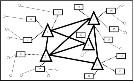
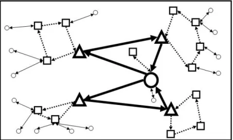
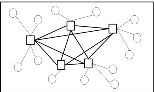
Since trucks and airplanes are included at the same time in the network, a hierarchical multimodal network is considered. The proposed network is a three layered hierarchical multimodal network. This hierarchical multimodal network has two different types of hubs which are ground hubs and airport hubs. Figure 2.4 shows a hierarchical multimodal network with 18 hubs. In this network, nodes 0-4 are the airport hubs; nodes 5-17 are the ground hubs and little circles with no numbers represent the demand points. In this representation, airline segments are illustrated as the thick lines between nodes 0-4; highway segments are illustrated with the thin lines between demand nodes and hubs (ground hubs or airport hubs), and with dashed lines between ground hubs and airport hubs.

(23)

11

Figure 2.4: Representation of a Multimodal Hierarchical Network

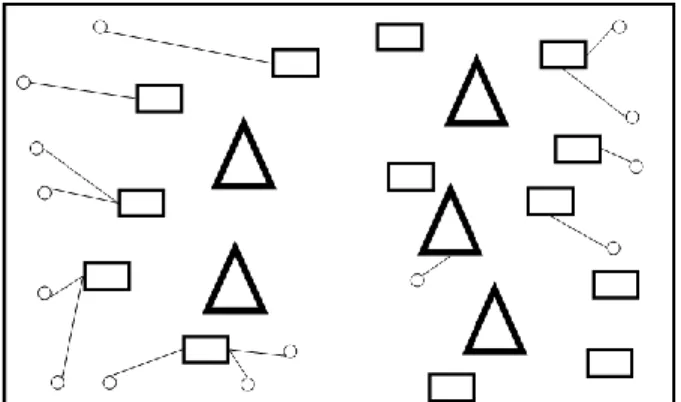
The third layer of the network consists of the allocations of demand points to the ground hubs and airport hubs (Figure 2.5(a)). At this layer, a star structure is used for the allocation of demand points. Each demand node is connected to exactly one hub (a ground or an airport hub) with a highway link. On these highway segments, pickup trucks are used.

The second layer includes the allocation of ground hubs to the airport hubs (Figure 2.5(b)). At the second layer, a star structure is considered for the allocation of the ground hubs, as well. Each ground hub is connected to exactly one airport hub with a highway link. Big trucks, which are faster and have more capacity than pickup trucks, are used at these highway segments and so economies of scale is considered.

(24)

12

(a) Third Layer

(b) Second Layer

(c) First Layer

(25)

13

A mesh structure is considered at the first (top) layer (Figure 2.5(c)). Airport hubs are connected with each other with an airline segment. On these airline segments, airplanes are considered.

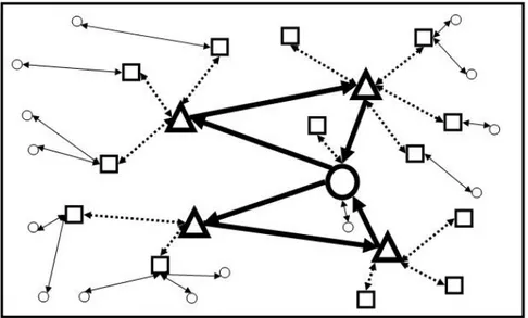
As we stated earlier; one of the aims of this study is to decrease the number of vehicles by changing the structure of the network. If a mesh structure is considered for the top layer of the hierarchy, high number of airplanes is required. Therefore, instead of a mesh hub network, another type of network topology can be used. Since the main aims are to decrease the number of airplanes and so to increase the utilization of the airplanes on hand, ring structure(s) can be efficient for the structure at the top layer. Therefore, ring structure(s) is considered at the top layer of hierarchy (Figure 2.6). This network is called as Ring(s)-Star-Star (R-S-S) network. In order to construct the ring structure(s), routing and scheduling decisions must be considered together. In other words, Vehicle Routing Problem (VRP) is considered at the top layer.

Figure 2.6: Ring(s)-Star-Star Network

With the rings structure at the top layer, the route of the airplane is decided while covering all origin-destination pairs in a given time bound. Tours are considered in the

(26)

14

routing decisions. In this study, we consider “first pick then deliver” type of service, which means that there are two separate tours. One of them is pickup tour(s) and the other is delivery tour(s). Initially, in the pickup tour(s), all demands are picked from their origins and they are sent to a specific airport hub. In these tours, there is no delivery. After all demands arrive at this airport hub, then in the delivery tour(s), all demands are sent to their final destinations. Since we need a specific airport hub in order collect all demands at one point, one of the airport hubs is assigned as the central airport hub. In Figure 2.6, central airport hub is represented as a big circle instead of triangle. If one airplane is not enough to cover all origin-destination pairs, there can be more than one airplane which travels among the airport hubs by drawing circles. Therefore, ring(s) can be constructed.

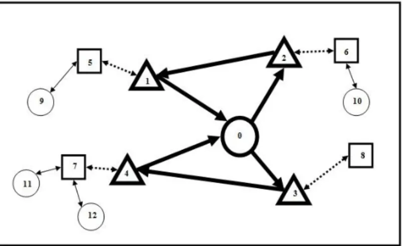
For the “first pick then deliver” type of service that we analyze, picking up from the origin and delivering to the destinations must be symmetrical. Therefore, the route of the delivery tour(s) is the reverse route of the pickup tour(s). In order to show the necessity of the reverse ordering, an example is analyzed in detail. Consider Figure 2.7. The hubs and demand nodes are numbered so that the central airport hub is 0, the airport hubs are from 1 to 4, the ground hubs are numbered from 5 to 8, and finally, demand nodes are from 9 to 12. In this example, we assume that all travel times between connected nodes are 1, except the travel time between 7 and 11, which is assumed to be 2. Then, we calculate the release times for all vehicles at the hubs. Based on the network at the Figure 2.7, at time 4, all demands are at the central airport hub and so at time 8, all demands can be delivered to their destination. Let us consider the flow from 10 to 11 in more detail. The cargo will travel along the path 10-6-2-1-0 in its pick-up tour and arrives at the central airport hub at time 4. Then, it will be loaded on the airplane 0-4-3-0 to be unloaded at node 4 at time 5. Finally, it will travel along the path 4-7-11 with the arrival time of 8. Now consider the case where the delivery route is in the same order of the pick-up route (instead of the reverse one). Again, the cargo will travel along the path

(27)

15

10-6-2-1-0 in its pick-up tour and arrives at the central airport hub at time 4. Then, it will be loaded on the airplane 0-3-4-0 to be unloaded at node 5 at time 6. Finally, it will travel along the path 4-7-11 with the arrival time of 9, which is higher than the time bound 8. Therefore, in order to satisfy the time bound, delivery tour(s) must be reverse of the pick-up tour(s).

Figure 2.7: Pick-up Tour(s)

Since all origin-destination pairs must be covered in a given time bound, the tour of an airplane is also bounded by the time. Therefore, the flights of the airplane must be scheduled according to the time bound. The airplane(s) must complete the flights in half of the time bound for pickup tour so that they can complete delivery tours in the other half. Thus, we aim to utilize the airplane(s) by incorporating scheduling decisions. Based on the proposed hierarchical multimodal network, the problem with ring structure(s) at the top layer can be defined as follows, given a set of demand nodes, a set of possible locations for ground hubs, a set of possible locations for airport hubs, the location of the central airport hub, the number of hubs to be located, the time bound and the travel time parameters; our proposed problem determines the location of ground hubs and airport hubs, the allocation of demand nodes to the hubs (ground or air), the allocation of the ground hubs to the airport hubs and the location of airline segments

(28)

16

while ensuring that all origin-destination pairs can be served in the given time bound. In the objective function, number of total flights (airline segments) is minimized.

Similar to the ring structure(s) of the top layer, another ring structure(s) can be considered at second layer as well in order to decrease the number of the big trucks and to increase the utilization of the big trucks on hand (Figure 2.8). This topology is referred to as Ring(s)-Ring(s)-Star (R-R-S) network. With that configuration, when ring structure is considered on the second layer, routing and scheduling decisions are included at that layer, too. Therefore, in this problem, routings are considered for both top and second layer of this hierarchical network.

Figure 2.8: Ring(s)-Ring(s)-Star Network

Based on this hierarchical multimodal network, this problem is similar to the R-S-S problem. In this one, the locations of highway segments between hubs are also decided and in the objective function, the weighted sum of the number of flights and number of road trips (highway segments) is minimized.

(29)

17

Chapter 3

Literature Review

In this chapter, we review the hub location literature in four main categories. The first one is devoted to the pioneering works of the classical hub location problem. In this section, basic assumptions of the hub location problem are stated. In the following sections, some of these assumptions are relaxed and new problems based on the relaxed assumption are explained. The second part is based on the studies on the hub location problem with incomplete network structure. The third one is related to the literature on the hub location problem with ring structure(s). In the fourth part, the literature on the hub location problem with multimodal network is presented. Finally, the literature on the hierarchical hub location problem is reviewed. Also, the study on the hub location problem with both hierarchical and multimodal network is analyzed.

(30)

18

3.1 The Standard Hub Location Problems

The research interest in hub location problem is started with the studies of O’Kelly [1, 2, 3]. He basically defines this problem as follows; given a set of demand nodes, positive flow between origin-destination pairs and the required number of hubs, the hub location problem consists of two main decisions, which are the locations of hubs and the allocation of demand nodes to these hubs.

O’Kelly [3] presented the first mathematical formulation for the hub location problem. In this formulation, the objective is minimizing the transportation cost while satisfying the flow balance. Flow is considered as airline passengers. This first mathematical formulation in the hub location literature is later categorized as single allocation p-hub median problem. There are three main assumptions for this problem. First, the hubs in the network are fully interconnected. Second, there is economies of scale, which means there is a discount factor (α) for hub-hub links. Finally, there is no direct link between non-hub nodes.

Let 𝑊_𝑖𝑗 be the flow between demand nodes i and j, and 𝐶_𝑖𝑗 be the transportation cost of a unit of flow between demand nodes i and j, define 𝑥_𝑖𝑘 as 1 if demand node i is allocated to the hub k, and 0 otherwise. In this situation, 𝑥_𝑘𝑘 is 1, if demand node k is a hub and 0, otherwise. The first integer programming formulation for the single allocation p-hub median problem proposed by O’Kelly [3] is as follows;

Minimize 𝑤𝑖𝑗 𝑗 𝑖 𝑐_𝑖𝑘𝑥_𝑖𝑘 𝑘 + 𝑐_𝑗𝑚𝑥_𝑗𝑚 𝑚 + 𝛼 𝑐_𝑘𝑚𝑥_𝑖𝑘𝑥_𝑗𝑚 𝑚 𝑘 (3.1) subject to 𝑛 − 𝑝 + 1 𝑥_𝑘𝑘 − 𝑥𝑖𝑘 𝑖 ≥ 0 _{∀ 𝑘} _(3.2)

(31)

19 𝑥_𝑖𝑘 𝑘 = 1 _{∀ 𝑖} _(3.3) 𝑥_𝑘𝑘 𝑘 = 𝑝 _(3.4) 𝑥_𝑖𝑘 ≥ 0 ∀ 𝑖, 𝑘 (3.5)

In the above formulation, the objective function (3.1) calculates the transportation cost. This objective function is quadratic because of the fact that hub-to-hub link is a product of two allocation decisions. Constraint (3.2) ensures that no demand node is allocated to a non-hub node. Also, Skorin-Kapov et al. [12] suggested that constraint (3.2) can be replaced with:

𝑥_𝑖𝑘 ≤ 𝑥_𝑘𝑘 ∀ 𝑖, 𝑘 (3.6)

Constraints (3.3) and (3.5) ensure that every demand node must be allocated to exactly one hub. Constraint (3.4) ensures that number of hubs to be open is p.

Due to the quadratic nature of the objective function, the hub location problems differ from the classical location problems. In classical location problem, each demand node is allocated to the nearest facility. However, in the hub location problem, nearest allocation strategy may not give the optimal solution. Therefore, allocation decisions of demand nodes must also be determined.

Based on the classification of the hub location problem made by Campbell [4], the hub location problem consists of the p-hub median problem, the hub location problem with fixed costs, the p-hub center problem and hub covering problems.

(32)

20

3.1.1 The p-hub Median Problem

In the p-hub median problem, the objective is to minimize the total transportation cost while satisfying the flow balance between origin-destination pair and also ensuring that the number of hubs to locate is p.

Campbell [4] presented the first linear integer programming formulation for the single allocation p-hub median problem. Later, Skorin-Kapov et al. [12] proposed a new mixed integer formulation for this problem, which gives tighter LP relaxation bounds. However, large size problems cannot be solved with this formulation. Then, Ernst and Krishnamoorthy [13] produced a different linear integer programming formulation with fewer decision variables and constraints in order to solve larger problems. They reduced the size of the problem by considering transfers among hubs as a multicommodity flow problem. Kara [14] proved that the p-hub median problem is NP-hard. In order to solve this problem, also some heuristic approaches are considered by Skorin-Kapov and Skorin-Kapov [15], Campbell [16], Ernst and Krishnamoorthy [13, 17] and recently Ilic et al. [18].

3.1.2 The Hub Location Problem with Fixed Costs

In this problem, in addition to the total transportation cost, fixed cost of opening a hub is also included into objective function. O’Kelly [19] proposed the first formulation for the single allocation hub location problem with fixed costs. This formulation is in a quadratic integer form. Since the number of hub is not fixed, the capacitated and uncapacitated versions of this problem are considered. Campbell [4] presented the first linear programming formulation for the single allocation uncapacitated and capacitated hub location problem with fixed costs. For the capacitated version, Ernst and Krishnamoorthy [20] produced a new formulation, which is based on the linear integer programming formulation proposed by Ernst and Krishnamoorthy [13] for the p-hub

(33)

21

median problem. Heuristic approaches are studied by Abdinnour-Helm and Venkataramanan [21], Abdinnour-Helm [22], Topcuoglu et al. [23], Cunha and Silva [24] and Chen [25].

3.1.3 The p-hub Center Problem

The objective of the p-hub center problem is to minimize maximum transportation cost. Campbell [4] presented the first formulations for the different type of p-hub center problem. Kara and Tansel [26] proposed several linear formulations for the single allocation p-hub center problem. Ernst et al. [27] produced a new formulation for the single allocation p-hub center problem. This new formulation has more continuous variable, but fewer constraints than the formulation proposed by Kara and Tansel [26] and in terms of CPU time requirements, formulation developed by Ernst et al. [27] is better. Some heuristics are developed to solve this problem (see, e.g., Pamuk and Sepil [28], Meyer et al. [29] and Ernst et al. [27]).

3.1.4 Hub Covering Problem

In hub covering problems, the objective is to minimize the number of hubs to cover all demand while satisfying a budget constraint or a time bound constraint. Campbell [4] presented the first mixed integer formulations for the hub covering problems. Kara and Tansel [30] proposed various linear formulations for the single allocation hub set covering problem. Ernst et al. [31] developed a new formulation for this problem, which is based on the formulation proposed by Ernst et al. [27] for the p-hub center problem. In terms of CPU time requirements, formulation presented by Ernst et al. [31] performs better. Some heuristic approaches for the hub covering problem are Calik et al. [32] and Hwang and Lee [33].

For comprehensive surveys on hub location, we refer the reader to Campbell et al. [34], Alumur and Kara [35], Kara and Taner [36], and Campbell and O’Kelly [37].

(34)

22

3.2 The Hub Location Problem with Incomplete Hub Network

Structure

The classical hub location problem is two-level with complete-star structure (complete for hub allocations and star for allocations of demand points). In the complete hub structure, hubs are fully interconnected that is one of the basic assumptions of the hub location problem. In the hub location literature, there exist some studies that relax this assumption and consider the incomplete hub network.

O’Kelly and Miller [38] introduced the incomplete hub network design to the literature. Nickel et al. [39] consider the multiple allocation hub location problems for urban public transport network. In addition to the total transportation cost, they also minimize the fixed cost of hub links. Campbell et al. [40, 41] introduced the hub arc location problems to the literature. In this problem, rather than locating hub facilities, hub arcs are located. Yoon and Current [42] also study the multiple allocation hub location problem with an incomplete hub network. They minimize total transportation cost and fixed cost of locating hubs and hub links. Alumur et al. [43] focus on the single allocation hub location problems over the incomplete hub networks. They define the single allocation incomplete p-hub median, the incomplete hub location with fixed costs, the incomplete hub covering and the incomplete p-hub center network design problems and proposed mathematical formulations for these problems.

The hub location problem is also studied in the context of telecommunication networks. In these networks, objective is to minimize the total cost of locating hubs and hub links. Therefore, for telecommunication applications, incomplete hub network design is considered. Many different types of network topologies such as star, tree, ring, and path are studied in the literature. Klincewicz [44] presented a review on the different type of the network structure of the location problem.

(35)

23

3.3 The Hub Location Problem with Ring Structure(s)

Based on the type of the proposed network, ring structure(s) concept in the literature is reviewed. “Ring structure(s)” on the hub location problem is firstly presented by Nagy and Salhi [45] as the many-to-many hub location-routing problem. In this study, it is stated that many-to-many location-routing problem can be reduced to the classical hub location problem when routing problem is not considered. They presented a mixed integer programming formulation and they proposed some solution techniques to solve this problem. They presented a hierarchical heuristic, in which hub location is considered as a master problem and routing problems as subproblems. Routing problems are solved via neighborhood search heuristic proposed by Nagy and Salhi [46]. Liu et al. [47] presented a mixed truck delivery system which allows both hub-and-spoke shipments and direct shipments. A heuristic is developed to decide the mode of delivery (hub-and spoke or direct) and perform vehicle routing in both delivery modes. Wasner and Zäpfel [48] presented a multi-depot hub location vehicle routing model for network design of parcel services. This model can be seen as a location-routing problem with the decision of the location of hubs and depots, and decision of routes between hubs/depots and their allocated demand points. Hub location part of this problem differs from the classical hub location problem with two aspects. Firstly, in this model, there can be a direct shipment between two demand points. Second one is that transportation cost between two hubs depends on the number of transports between those two hubs. They presented a mixed integer optimization model. However, due to the complexity of this model, a heuristic, which is based on local search procedure, was developed. A case study for Austria, which consists of one possible hub location, ten possible depot locations and 2042 demand points, was conducted. Çetiner et al. [49] proposed the combined hub location-routing problem, which includes the hub location decisions and also routing decision between demand points. This problem is developed for the postal delivery system in Turkey. In this study, multiple-allocation is allowed and it is assumed

(36)

24

that the hubs and the vehicles are uncapacitated. An iterative two-stage heuristic is developed to solve this problem. In the first stage, hub locations and the allocation of non hub nodes are determined. In the second stage, routes between demand points are decided. After the second stage, the distances between demand points are updated in order to solve the new hub location problem. Camargo et al. [50] presented a new formulation to the many-to-many hub location-routing problem. In this formulation, single allocation and uncapacitated hubs and vehicles are considered. The completion of a tour is bounded by a service level and each costumer is visited exactly once. They solve the problem by using Benders decomposition algorithm. With this algorithm, large-size instances (up to 100 nodes) of this problem can be solved optimally.

3.4 The Hub Location Problem with Multimodal Network

Structure

In the standard hub location problem, the mode decisions for type of transportation vehicles are not considered. The main assumption is that there are two transportation modes. One of them is between hubs and the other one is between hubs and non-hubs. In the literature, some researchers extend their study by considering transportation mode decisions in addition to location and allocation decisions and also by increasing number of transportation modes.

The first study of the hub location problem including the choice for transportation mode is proposed by O’Kelly and Lao [51]. In this study, there are two fixed hub locations, which are mini-hub and master-hub. This problem is solved by addressing two sub-problems. The first one is the decision of transportation mode (air or truck) while satisfying given time limitations. The second one is the allocation decision of cities to the mini-hub. Multimodal hub location and hub network design problem is first introduced by Alumur et al. [52]. In this study, in addition to the decisions of the

(37)

25

classical hub location problem, decision of the transportation mode is also considered. They presented a linear mixed integer programming model and they considered the different variants of this problem. Also, several valid inequalities and a heuristic are proposed.

3.5 The Hierarchical Hub Location Problem

As we mentioned before that classical hub location problem has two level structures. However, some studies relax that assumption and consider the hub network structure more than two levels. This type of network structure is referred as the hierarchical hub network.

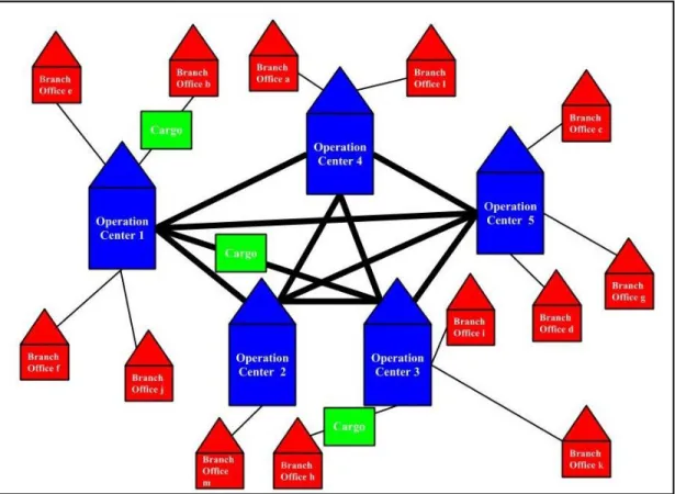
Smilowitz and Daganzo [53] focus on the design of integrated package distribution systems for multiple transportation modes and multiple service level delivery network. They consider separate networks for each mode. For ground and air transportation mode, they propose ring(s)-ring(s)-complete and ring(s)-ring(s)-tree networks, respectively. They used continuum approximation approach to minimize the cost. Yaman [54] proposes a three level hub network, which consists of complete network at top level and star networks at the second and third level, is presented. According to its objective, this problem is considered as the hierarchical hub median problem. She also studies a different version of this problem by considering the service level quality. The author proposes a mixed integer programming model. Sahraeian and Korani [55] consider the same three level hub network structure as Yaman [54] did. However, they propose the maximal covering problem version with given cover radii.

Also, some researchers study both multimodal and hierarchical hub network structure together. Alumur et al. [10] presented a hierarchical multimodal hub location problem with time definite deliveries. In this study, a star-incomplete-star network with air and ground transportation mode is considered. They proposed a mixed integer programming

(38)

26

and a set of valid inequalities. In the mathematical model, they minimize the total transportation and operational costs.

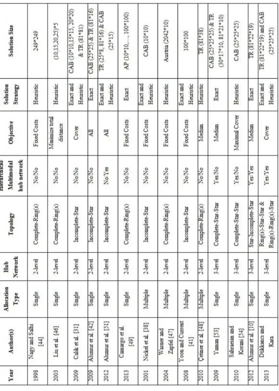
In our study, a hub covering problem is proposed. Since we consider ring structure(s) at the top (and also second) layer(s), the proposed hub network is incomplete. Also, the hub network is multimodal and hierarchical. The similarities and differences between the proposed problem and the related hub location problems in the literature can be seen in the Table 3.1.

(39)

27

(40)

28

Chapter 4

Model Formulations

In this chapter, we formulate the hierarchical hub location problem with three layered structure. The organization of this chapter is as follows. Section 4.1 provides the mathematical formulation of the hierarchical hub location problem on a ring(s)-star-star (R-S-S) network. In addition to the mathematical formulation, some valid inequalities are proposed. In Section 4.2, the hierarchical hub location problem on a ring(s)-ring(s)-star (R-R-S) network is formulated.

(41)

29

4.1 The Hierarchical Hub Location Problem on a

Ring(s)-Star-Star Network

In this problem, the hierarchical hub network is based on the R-S-S structure (Figure 4.1).

4.1.1 Problem Formulation

We propose a linear mixed integer mathematical model for the proposed problem. Given the node set, potential ground hub and airport hub locations, the model outputs the network configuration with ground hubs, airport hubs, the allocations of demand points to the ground or airport hubs and the allocations of ground hubs to the airport hubs, and the required airline segments with the minimum number of airline links while obeying the time bound.

Let D be the set of demand points, H be the set of possible hub locations (H⊆ D), A be the set of possible airport hub locations (A⊆ H), and 0 be the central airport hub (0 ∈ A). Also, it is assumed that travel time data is symmetrical and satisfies triangular inequality.

The parameters of our mathematical model are as follows; p = number of hubs

𝑡_𝑖𝑗 = travel time from node i ∈ D to node j ∈ D by truck

𝑡_𝑖𝑗𝑎𝑖𝑟= travel time from node i ∈ D to node j ∈ D by airplane α = discount factor of time for ground transportation

𝑚𝑙= loading-unloading time at airport l ∈ A

𝑇 = time bound for each origin-destination pair

M = maximum travel time between a ground hub and an airport hub plus loading-unloading time at that airport

(42)

30

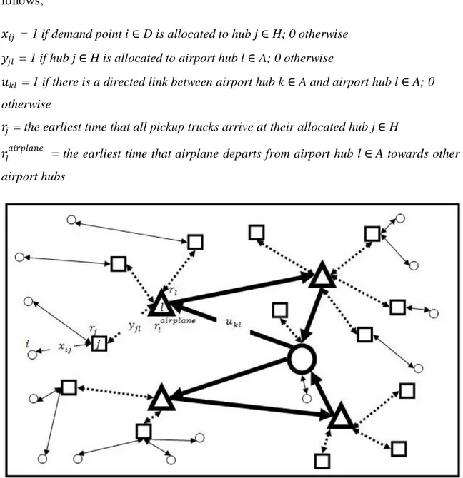
The decision variables of our mathematical model also depicted in Figure 4.1 are as follows;

𝑥_𝑖𝑗 = 1 if demand point i ∈ D is allocated to hub j ∈ H; 0 otherwise 𝑦_𝑗𝑙 = 1 if hub j ∈ H is allocated to airport hub l ∈ A; 0 otherwise

𝑢_𝑘𝑙 = 1 if there is a directed link between airport hub k ∈ A and airport hub l ∈ A; 0 otherwise

𝑟_𝑗 = the earliest time that all pickup trucks arrive at their allocated hub j ∈ H

𝑟_𝑙𝑎𝑖𝑟𝑝𝑙𝑎𝑛𝑒 = the earliest time that airplane departs from airport hub l ∈ A towards other airport hubs

Figure 4.1: R-S-S Network

(43)

31 (R-S-S) Minimize 𝑢𝑘𝑙 𝑙∈𝐴\{𝑘} 𝑘∈𝐴 (4.1) subject to 𝑥_𝑖𝑘 𝑘 = 1 _{∀ 𝑖} _(3.3) 𝑥𝑘𝑘 𝑘 = 𝑝 _(3.4) 𝑥_𝑖𝑘 ≤ 𝑥_𝑘𝑘 ∀ 𝑖, 𝑘 (3.6) 𝑦𝑗𝑙 𝑙∈𝐴 = 𝑥𝑗𝑗 _{∀ 𝑗 ∈ 𝐻} _(4.2) 𝑦_𝑗𝑙 ≤ 𝑦_𝑙𝑙 ∀ 𝑗 ∈ 𝐻, 𝑙 ∈ 𝐴 (4.3) 𝑦_𝑗𝑗 ≤ 𝑥_𝑗𝑗 ∀ 𝑗 ∈ 𝐴 (4.4) 𝑦00 = 1 (4.5) 𝑢_𝑘𝑙 𝑙∈𝐴\{𝑘} = 𝑦_𝑘𝑘 _{∀ 𝑘 ∈ 𝐴} _(4.6) 𝑢𝑙𝑘 𝑙∈𝐴\{𝑘} = 𝑦𝑘𝑘 _{∀ 𝑘 ∈ 𝐴} _(4.7) 𝑢_0𝑙 𝑙∈𝐴\{0} = 𝑢_𝑙0 𝑙∈𝐴\{0} (4.8) 𝑟𝑗 ≥ 𝑡𝑖𝑗𝑥𝑖𝑗 ∀ 𝑖 ∈ 𝐷, 𝑗 ∈ 𝐻 (4.9) 𝑟_𝑙𝑎𝑖𝑟𝑝𝑙𝑎𝑛𝑒 ≥ 𝑟_𝑗 + 𝛼𝑡_𝑗𝑙 + 𝑚_𝑙 𝑦_𝑗𝑙 − 𝑀(1 − 𝑦𝑗𝑙) ∀ 𝑗 ∈ 𝐻, 𝑙 ∈ 𝐴\ 𝑗 (4.10) 𝑟_𝑘𝑎𝑖𝑟𝑝𝑙𝑎𝑛𝑒 − 𝑟_𝑙𝑎𝑖𝑟𝑝𝑙𝑎𝑛𝑒 + 𝑇𝑢_𝑘𝑙 ≤ 𝑇 − (𝑡_𝑘𝑙𝑎𝑖𝑟 + 𝑚_𝑙)𝑢_𝑘𝑙 ∀ 𝑘 ∈ 𝐴\ 0 , 𝑙 ∈ 𝐴\ 𝑘 (4.11) 𝑟_𝑘𝑎𝑖𝑟𝑝𝑙𝑎𝑛𝑒 ≥ (𝑡_0𝑘𝑎𝑖𝑟 + 𝑚_𝑘)𝑢_0𝑘 ∀ 𝑘 ∈ 𝐴\ 0 (4.12) 2𝑟₀𝑎𝑖𝑟𝑝𝑙𝑎𝑛𝑒 ≤ 𝑇 (4.13)

(44)

32

𝑥_𝑖𝑘 ≥ 0 ∀ 𝑖, 𝑘 (3.5)

𝑦_𝑗𝑙 ∈ 0,1 ∀ 𝑗 ∈ 𝐻, 𝑙 ∈ 𝐴 (4.14)

𝑢_𝑘𝑙 ∈ 0,1 ∀ 𝑘 ∈ 𝐴, 𝑙 ∈ 𝐴\ 𝑘 (4.15)

𝑟_𝑙𝑎𝑖𝑟𝑝𝑙𝑎𝑛𝑒 ≥ 0 ∀ 𝑙 ∈ 𝐴 (4.16) The objective function (4.1) minimizes the operational cost of airline links between airport hubs. Observe here that, multiplying each link with a parameter, one can easily convert this function to operational cost.

The Constraints (3.3)-(3.6) are the classical hub location constraints as explained in the Chapter 2. By Constraint (4.2), a hub is allocated to exactly one airport hub. Constraint (4.3) guarantees that no hub is allocated a non airport hub. That is, if a hub is allocated to an airport hub, then this airport hub must be opened. Due to Constraint (4.4), if an airport hub is established in a node, then in this node, a hub must be opened. Constraint (4.5) establishes the central airport hub. Constraints (4.6) and (4.7) construct the ring structure(s) for the airport hubs (top layer of the hierarchical network). Constrains (4.8) allows to structure with more than one ring, which means that there can be more than one airplane, if necessary.

Constraint (4.9) calculates the earliest time that pickup trucks arrive at their allocated hub. Constraint (4.10) determines the earliest time that all pickup trucks from demand points and big trucks from ground hubs, which are allocated to the same airport hub, arrive at that airport hub. With Constraint (4.11), we ensure that the earliest time that an airplane departs from any airport hub is within predetermined time bound. We remark here that Constraint (4.11) also acts as sub-tour breaking constraints. Constraint (4.12) calculates the earliest time that airplane departs from the airport hub, which has a directed link from the central airport hub. We compute this time separately in order to complete ring structure(s) for the top layer. By Constraints (4.13), we guarantee that all origin-destination pairs are covered in a given time bound. Since we assume the

(45)

33

symmetric travel time data, we consider the pickup and delivery as the same, so we multiply by 2. Finally, constraints (4.14) – (4.16) are the domain constraints

This mathematical model is a mixed binary programming model with O(n2_{) binary}

variables, O(n) non-negative variables, and O(n2_{) constraints.}

4.1.2 Valid Inequalities

In this section, some valid inequalities are presented. These valid inequalities are based on the time restriction.

Actually, the first one is a variable fixing rule, which can be included into the model as pre-processing. However, in our model, we consider it as a valid inequality. For i ∈ D and j ∈ H\{i}, if 𝑡_𝑖𝑗 _{> 𝑇 2} , then demand node i cannot be allocated to the hub (ground or airport) j, since travel time between the city i and city j exceeds half of the time bound T. Therefore, the inequality

𝑡_𝑖𝑗 _{− 𝑇 2} 𝑥_𝑖𝑗 ≤ 0 ∀ 𝑖 ∈ 𝐷, 𝑗 ∈ 𝐻\{𝑖} (4.17)

is valid. With Constraint (4.17), if 𝑡_𝑖𝑗 _{> 𝑇 2} , then 𝑥_𝑖𝑗 will be equal to 0 that means demand node i cannot be assigned to hub j.

For i ∈ D, j ∈ H\{i} and l ∈ A\{i,j}, if 𝑡_𝑖𝑗 + 𝛼 ∗ 𝑡_𝑗𝑙 + 𝑚_𝑙 _{> 𝑇 2} , then demand node i cannot be allocated to the ground hub j and ground hub j cannot be allocated to the airport hub l at the same time. Therefore, the inequality

𝑥_𝑖𝑗 + 𝑦_𝑗𝑙 ≤ 1 ∀ 𝑖 ∈ 𝐷, 𝑗 ∈ 𝐻\{𝑖}, 𝑙 ∈ 𝐴\{𝑖, 𝑗}, 𝑖𝑓 𝑡_𝑖𝑗 + 𝛼 ∗ 𝑡_𝑗𝑙 + 𝑚_𝑙 _{> 𝑇 2} (4.18) is valid. With Constraint (4.18), if travel from demand node i to the airport hub l through ground hub j exceeds the half of the time bound, then 𝑥_𝑖𝑗 and 𝑦_𝑗𝑙 will not be equal to 1 at the same time.

(46)

34

The performances of these two valid inequalities are explained in detail in Chapter 5.

4.2 The Hierarchical Hub Location Problem on a

Ring(s)-Ring(s)-Star Network

This problem considers the hierarchical hub location on the R-R-S network. In this network, the second layer also consists of ring(s) (Figure 4.2).

Figure 4.2: R-R-S Network

4.2.1 Problem Formulation

For this problem, a linear mixed integer mathematical model is presented. Given the node set, potential ground hub and air hub locations, the model outputs the network configuration with ground hubs, airport hubs, the allocations of demand points to the ground or airport hubs and the allocations of ground hubs to the airport hubs, and the

(47)

35

required airline and highway segments with the minimum number of airline and highway links while obeying the time bound.

Let D be the set of demand points, H be the set of possible hub locations (H ⊆ D), A be the set of possible airport hub locations (A ⊆ H), and 0 be the central airport hub (0 ∈ A). The parameters and decision variables explained in Section 4.1.1 are also valid for this problem. The additional parameters and variables are as follows;

β = coefficient for airline segments between airport hubs

γ = coefficient for ground segments between hubs (ground or air)

𝑧_𝑗𝑘𝑙 = 1 if there is a directed link between hub j ∈ H and hub k ∈ H and these two hubs

are allocated to the same airport hub l ∈ A

𝑟_𝑙𝑏𝑖𝑔𝑡𝑟𝑢𝑐𝑘 = the earliest time that big truck departs from hub l ∈ H towards other hubs The mixed integer programming formulation of the proposed problem is as follows;

(R-R-S) Minimize 𝛽 𝑢𝑘𝑙 𝑙∈𝐴\{𝑘} 𝑘 ∈𝐴 + 𝛾 𝑧_𝑗𝑘𝑙 𝑙∈𝐴 𝑘 ∈𝐻\{𝑗 } 𝑗 ∈𝐻 (4.19) subject to 𝑥_𝑖𝑘 𝑘 = 1 _{∀ 𝑖} _(3.3) 𝑥_𝑘𝑘 𝑘 = 𝑝 _(3.4) 𝑥_𝑖𝑘 ≤ 𝑥_𝑘𝑘 ∀ 𝑖, 𝑘 (3.6) 𝑦_𝑗𝑙 𝑙∈𝐴 = 𝑥_𝑗𝑗 _{∀ 𝑗 ∈ 𝐻} _(4.2) 𝑦_𝑗𝑙 ≤ 𝑦_𝑙𝑙 ∀ 𝑗 ∈ 𝐻, 𝑙 ∈ 𝐴 (4.3) 𝑦_𝑗𝑗 ≤ 𝑥_𝑗𝑗 ∀ 𝑗 ∈ 𝐴 (4.4)

(48)

36 𝑦₀₀ = 1 (4.5) 𝑢_𝑘𝑙 𝑙∈𝐴\{𝑘} = 𝑦_𝑘𝑘 _{∀ 𝑘 ∈ 𝐴} _(4.6) 𝑢_𝑙𝑘 𝑙∈𝐴{𝑘} = 𝑦_𝑘𝑘 _{∀ 𝑘 ∈ 𝐴} _(4.7) 𝑢_0𝑙 𝑙∈𝐴\{0} = 𝑢_𝑙0 𝑙∈𝐴\{0} (4.8) 𝑧_𝑗𝑘𝑙 𝑗 ∈𝐻\{𝑘} = 𝑦_𝑘𝑙 _{∀ 𝑘 ∈ 𝐻, 𝑙 ∈ 𝐴\ 𝑘} _(4.20) 𝑧_𝑘𝑗𝑙 𝑗 ∈𝐻\{𝑘} = 𝑦_𝑘𝑙 _{∀ 𝑘 ∈ 𝐻, 𝑙 ∈ 𝐴\ 𝑘} _(4.21) 𝑧_𝑗𝑙𝑙 𝑗 ∈𝐻\{𝑙} = 𝑧_𝑙𝑗𝑙 𝑗 ∈𝐻\{𝑙} _{∀ 𝑙 ∈ 𝐴} _(4.22) 𝑟_𝑗 ≥ 𝑡_𝑖𝑗𝑥_𝑖𝑗 _{∀ 𝑖 ∈ 𝐷, 𝑗 ∈ 𝐻} (4.9) 𝑟_𝑘𝑎𝑖𝑟𝑝𝑙𝑎𝑛𝑒 − 𝑟_𝑙𝑎𝑖𝑟𝑝𝑙𝑎𝑛𝑒 + 𝑇𝑢_𝑘𝑙 ≤ 𝑇 − (𝑡_𝑘𝑙𝑎𝑖𝑟 + 𝑚_𝑙)𝑢_𝑘𝑙 ∀ 𝑘 ∈ 𝐴\ 0 , 𝑙 ∈ 𝐴\ 𝑘 (4.11) 𝑟_𝑘𝑎𝑖𝑟𝑝𝑙𝑎𝑛𝑒 ≥ (𝑡_0𝑘𝑎𝑖𝑟 + 𝑚_𝑘)𝑢_0𝑘 _{∀ 𝑘 ∈ 𝐴\ 0} (4.12) 𝑟_𝑗𝑏𝑖𝑔𝑡𝑟𝑢𝑐𝑘 − 𝑟_𝑘𝑏𝑖𝑔𝑡𝑟𝑢𝑐𝑘 + 𝑇𝑧_𝑗𝑘𝑙 ≤ 𝑇 − 𝛼𝑧_𝑗𝑘𝑙 𝑡_𝑗𝑘 ∀ 𝑙 ∈ 𝐴, 𝑗 ∈ 𝐻\{𝑙}, 𝑘 ∈ 𝐻\{𝑗} (4.23) 𝑟_𝑗𝑏𝑖𝑔𝑡𝑟𝑢𝑐𝑘 ≥ 𝛼𝑡_𝑙𝑗𝑧_𝑙𝑗𝑙 ∀ 𝑗 ∈ 𝐻, 𝑙 ∈ 𝐴\{𝑗} (4.24) 𝑟_𝑗𝑏𝑖𝑔𝑡𝑟𝑢𝑐𝑘 ≥ 𝑟_𝑗 _{∀ 𝑗 ∈ 𝐻} (4.25) 𝑟_𝑘𝑎𝑖𝑟𝑝𝑙𝑎𝑛𝑒 ≥ 𝑟_𝑘𝑏𝑖𝑔𝑡𝑟𝑢𝑐𝑘 + 𝑚_𝑘 ∀ 𝑘 ∈ 𝐴 (4.26) 2𝑟₀𝑎𝑖𝑟𝑝𝑙𝑎𝑛𝑒 ≤ 𝑇 (4.13) 𝑥_𝑖𝑘 ≥ 0 ∀ 𝑖, 𝑘 (3.5) 𝑦𝑗𝑙 ∈ 0,1 ∀ 𝑗 ∈ 𝐻, 𝑙 ∈ 𝐴 (4.14) 𝑢_𝑘𝑙 ∈ 0,1 ∀ 𝑘 ∈ 𝐴, 𝑙 ∈ 𝐴\ 𝑘 (4.15)

(49)

37

𝑧_𝑗𝑘𝑙 _{∈ 0,1} _{∀ 𝑗 ∈ 𝐻, 𝑘 ∈ 𝐻\{𝑗}, 𝑙 ∈ 𝐴} _(4.27)

𝑟_𝑙𝑎𝑖𝑟𝑝𝑙𝑎𝑛𝑒 ≥ 0 ∀ 𝑙 ∈ 𝐴 (4.17) 𝑟_𝑙𝑏𝑖𝑔𝑡𝑟𝑢𝑐𝑘 ≥ 0 ∀ 𝑙 ∈ 𝐻 (4.28)

In this model, the objective function (4.19) minimizes the weighted sum of the operational cost of airline and highway segments among airport hubs and ground hubs (γ < β). Again, multiplying each link with a parameter, one can easily convert this function to operational cost.

Constraints (3.3)-(3.6); (4.2)-(4.9); (4.11)-(4.17) are from the R-S-S model. Constraints (4.20) and (4.21) construct the ring structure(s) for the ground hubs (second layer of the hierarchical hub network). Constrains (4.22) allows to structure with more than one ring for one airport hub, which means that there can be used more than one big truck, if necessary.

With Constraint (4.23), we ensure that the earliest time that a big truck departs from any ground hub is within predetermined time bound. Also, we remark that Constraint (4.23) acts as sub-tour breaking constraints for the big truck tours. Constraint (4.24) calculates the earliest time that a big truck departs from the ground hub, which has a directed link from its allocated airport hub. We compute this time separately in order to complete ring structure(s) for the second layer. Constraint (4.25) ensures that a big truck departs from the hub, after the arrival of all demands from its demand nodes. Constraint (4.26) guarantees that an airplane departs from the airport hub, after the arrival of all demands from its ground hubs and loading of all demands to the airplane.

(50)

38

This mathematical model is a mixed binary programming model with O(n3_{) binary}

variables, O(n) non-negative variables, and O(n3_{) constraints.}

We remark here that; since we do not change star structure for the third layer, the two valid inequalities from the R-S-S model can be used for this model, too. So, Constraints (4.17) and (4.18) are also used for this model.

(51)

39

Chapter 5

Computational Settings and the

Performance of the Valid Inequalities

In this chapter, we present data sets for the computational studies and the performance of the proposed valid inequalities. The organization of this chapter is as follows. Section 5.1 presents two data sets and their settings. In Section 5.2 we evaluate the performance of the valid inequalities.

5.1 Data Sets

In our computational studies, we use two different data sets, which are Civil Aeronautics Board (CAB) and Turkish network (TR) data sets. CAB data set is based on the airline passenger interactions between 25 cities in United States in 1970. Initially, O’Kelly [3]

(52)

40

introduced this data set. Then, almost all of the hub location researchers used and referred CAB data set. Recently, a Turkish network introduced to literature by Tan and Kara [6]. This data set consists of 81 cities in Turkey as demand points. For data on the CAB and Turkish network data sets, the reader is referred to Beasley [56].

For Turkish network, we consider 81 cities of Turkey as demand points, 22 of 81 cities as potential ground hub and 19 of 22 cities as potential airport hub.

Figure 5.1: Turkey Map with cities and potential hub set

In Figure 5.1, numbers represent the city plate numbers of the 81 cities of Turkey. There are 22 potential hub nodes which are represented as circles. The 19 potential airport hubs are among these 22 nodes except Afyon (3), Aksaray (68) and Düzce (81) since there are not any airports in these cities. The central airport hub is considered as Ankara (6) due to its geopolitical advantageous location. Also, Ankara has the second biggest amount of flow in Turkey.

The time discount factor α is taken as 0.9. The distance data is taken from Tan and Kara [6]. The travel times are calculated by assuming that the trucks travel at a speed of 70 km/hr. Also, it is assumed that the airplanes travel at a speed of 700 km/hr. The loading/unloading time at an airport is taken as 30 minutes.

(53)

41

For R-R-S model, coefficients β and γ in the objective functions are taken as 10 and 5 in order to show the airline segments are more costly than the ground segments.

For CAB data set, we consider 25 cities of USA as demand points, potential ground and airport hubs.

Figure 5.2: USA Map with 25 cities

In Figure 5.2, 25 nodes represent the demand nodes, potential ground and airport hubs on the USA map. The central airport hub is assigned to Atlanta (1) since it can be considered as located in the center of most of the cities.

The distance data is taken from O’Kelly [3]. The other settings are the same as on the Turkish network.

Computational studies are carried on a server with 4 * AMD Opteron Interlagos 6282 SE and 96 GB of RAM and we used optimization software Gurobi version 5.0.2.