Exploring the Role of Loss Functions in
Multiclass Classification
Ahmet Demirkaya
Dept. of Electrical & Electronics Engineering Bilkent University
Istanbul, Turkey
Email: [email protected]
Jiasi Chen
Dept. of Computer Science & Engineering University of California, Riverside
Riverside, CA, USA Email: [email protected]
Samet Oymak
Dept. of Electrical & Computer Engineering University of California, Riverside
Riverside, CA, USA Email: [email protected]
Abstract—Cross-entropy is the de-facto loss function in modern classification tasks that involve distinguishing hundreds or even thousands of classes. To design better loss functions for new machine learning tasks, it is critical to understand what makes a loss function suitable for a problem. For instance, what makes the cross entropy better than other alternatives such as quadratic loss? In this work, we discuss the role of loss functions in learning tasks with a large number of classes. We hypothesize that different loss functions can have large variability in the difficulty of optimization and that simplicity of training is a key catalyst for better test-time performance. Our intuition draws from the success of over-parameterization in deep learning: As a model has more parameters, it trains faster and achieves higher test accuracy. We argue that, effectively, cross-entropy loss results in a much more over-parameterized problem compared to the quadratic loss, thanks to its emphasis on the correct class (associated with the label). Such over-parameterization drastically simplifies the training process and ends up boosting the test performance. For separable mixture models, we provide a separation result where cross-entropy loss can always achieve small training loss, whereas quadratic loss has diminishing benefit as the number of classes and class correlations increase. Numerical experiments with CIFAR 100 corroborate our results. We show that the accuracy with quadratic loss disproportionately degrades with a growing number of classes; however, encouraging quadratic loss to focus on the correct class results in a drastically improved performance.
Index Terms—cross entropy, multiclass classification, quadratic loss, over-parameterization, deep neural networks
I. INTRODUCTION
Modern machine learning problems involve complex tasks where one has to make the optimal decision given hundreds or thousands of possible actions. Hence multiclass classification lies at the heart of various application domains such as recom-mender systems, robotics, search engines, and computer vision. In state-of-the-art supervised learning problems, practitioners typically use large capacity deep neural networks together with cross-entropy loss [1], [2]. It is known that the true posterior probability is a global minimum for both the cross-entropy (CE) and quadratic (i.e. squared) loss (QL) [3], [4], [5]. Hence these loss functions are Bayes consistent and can implement Bayes optimal classification when combined with expressive models such as deep networks [6], [7]. However, QL is rarely used for multiclass problems. Our goal in this paper is to understand the role of the loss function on the classifier performance and
to shed light on what makes one loss function perform better than another.
Our key intuition is that the performance of modern classi-fiers is highly connected to the optimization landscape. Indeed in practice, deep neural networks are typically trained until they achieve 100% accuracy on the training data [8] and the network size is much larger than the size of the training dataset, i.e., the problem is over-parameterized. We have a growing understanding of the benefits of over-parameterization and how it simplifies the training process while often maintaining the accuracy [9], [10], [11], [12].
In this paper, we build on the importance of optimization landscape with an emphasis on loss functions. Via empirical observations and theoretical arguments, we argue that loss functions that are easier to train also generalize better. Over-parameterization is a crucial catalyst of simpler and faster training; however, it has been only studied in the context of a model having more parameters. We argue that different loss functions have different levels of effective overparam-eterization, which greatly affects the final performance. For instance, QL is inherently more determined (less over-parameterized) compared to CE. This results in an unfavorable optimization landscape and less tractable optimization problems. Intuitively, this stems from the fact that QL focuses on fitting all classes, whereas CE focuses on only the correct class (associated with the label), while maximizing the margin to the remaining classes.
Contributions. This paper makes the following contributions: ● We contrast the QL and CE for a mixture model with K components using linear classifiers. We show that CE can achieve arbitrarily small loss whereas QL has vanishing benefit as the class sizes and correlations increase. Normalized QL loss is lower bounded by 1 − r/K (compared to a reference of 1) where r is the subspace induced by the component centers. ● Numerical experiments on CIFAR 100 confirm the theory and demonstrate that increased number of classes hurts QL disproportionately. In particular, stochastic gradient descent (SGD) is unable to properly optimize QL with 100 classes despite over-parameterization.
● To highlight the importance of relaxing the loss function and over-parameterization, we propose a simple variant of QL which is encouraged to focus on the correct class, rather
than all classes as by default. This loss function consistently outperforms the default QL and can achieve full training accuracy and competitive test performance on CIFAR 100. Related work. Classification loss functions have a long history in statistics and machine learning [4], [13]. CE and QL have been compared in several interesting works [14], [15], [16]; however these works do not focus on the optimization landscape and large number of classes. Extreme multiclass problems with huge number of classes have been studied by [17], [18], [19]. For datasets with separable classes, recent works show that gradient descent converges to the max-margin solution with CE loss [20], [21]. Designing good loss functions is an active research topic [22], [23], [24].
Our insights relate to the recent literature on the benefits of over-parameterization. Recent works show that large-capacity deep networks have the ability to fit essentially any training dataset for both QL and CE loss [9], [25], [26]. This work highlights the loss function as an additional “control knob” and argues that QL is relatively less over-parameterized than CE.
II. PROBLEMSETUP
We first define the notation. We denote the number of classes by K. Let v[i] denotes the ith entry of a vector v ∈ RK. Given an integer k obeying 1 ≤ k ≤ K, we define a one-hot encoding one-one-hot(k) as follows: one-one-hot(k)[k] = 1 and one-hot(k)[`] = 0 for ` ≠ k. The softmax operator is denoted by sftmx(v) with entries sftmx(v)[k] = ev[k]
/∑Ki=1ev[i]. IK
denotes the identity matrix of dimensions K × K.
We consider the supervised classification problem with multiple classes. The joint distribution of the data is denoted by D. Given (x, y) ∼ D, we assume that the input vector obeys x ∈ Rd and label y ∈ {1, 2, . . . , K} is an integer corresponding to the true class assignment to one of the K classes.
Let f ∶ Rd→RKbe a multiclass classifier (e.g.,a deep neural network) that maps an input to a K dimensional vector of class predictions. At an input x, f outputs a hard decision arg max1≤k≤Kf (x)[k]. Hence test accuracy is given by:
L0−1(f, D) = Ex,y[y = arg max
1≤k≤Kf (x)[k]].
In the population limit (i.e., infinitely many training samples), QL is defined as: LQL(f, D) = 1 2Ex,y[∥one-hot(y) − f (x)∥ 2 `2].
Cross-entropy loss is calculated after the application of the softmax layer and is given by:
LCE(f, D) = − Ex,y[log(sftmx(f (x))[y])]
Note that QL attempts to fit all classes, i.e., it sets the correct class to one and other classes to zero. In contrast, CE focuses mostly on the correct class and is more ignorant of the predictions made on other classes. The impact of all remaining class predictions are summarized using a single number in softmax given by ∑i≠yef (x)[i]. Hence, CE
inher-ently aims to maximize the margin between the correct class and the remaining classes, where the margin is defined as
marginf(y, x) = f (x)[y] − maxi≠yf (x)[i]. In particular, as
soon as all training examples achieve positive margins, CE training loss can be pushed to zero by using the scaled classifier αf and letting α → ∞.
Towards demonstrating the benefit of focusing on the correct class, we will also consider a modification of QL which puts more emphasis on the correct class. We call this Correct-Class Quadratic-Loss (CCQL), defined as:
LCCQL(f, D) = LQL(f, D) +
w
2 E[(1 − f (x)[y])
2
] (II.1) This modified QL is parameterized by w which controls the amount of emphasis on the correct class. In the extreme scenario of w → ∞, CCQL ignores all other classes and reduces to minimizing E[(1 − f (x)[y])2]. Note that this is not a good idea as a non-informative classifier always predicting the all ones vector would achieve zero loss. We will use CCQL in our experiments to demonstrate that emphasizing correct class does indeed help training.
Finally, our analysis in the next section will consider a linear classifier parameterized by Θ ∈ RK×d, i.e.m f (x) = f (x, Θ) = Θx. We remark that technical arguments can potentially be extended to kernels or even neural nets [9], [25], [26] by using high-dimensional feature maps x → φ(x) and studying the linear classifier in the feature space, i.e., f (x) = Θφ(x).
III. COMPARISON OFLOSSFUNCTIONS ONMIXTURE
MODELS
This section presents results comparing CE, QL and CCQL on a simple distribution (mixture model) from a theoretical point of view. Our mixture model has K classes as described below.
Definition 3.1 (K-class Mixture): A sample (x, y) ∼ D from a mixture model distribution D is generated as follows. Let (µk)Kk=1 be the K component centers satisfying ∥µk∥`2 = 1
and, for some γ > 0, let:
∣µTiµj∣ ≤1 − 3γ for any i ≠ j
Each label y is equally likely, i.e., E[y = k] = 1/K. Conditional distribution x − µysatisfies E[x − µy] =0 and E[(x − µy)(x − µy)T] =σ2Id. If we additionally have ∥x − µy∥`2 ≤γ, then
Dis called a Bounded Mixture Model.
●CE Loss: We first consider a linear classifier with the CE loss. Leveraging the margin γ between the classes, it is fairly straightforward to show that CE loss can be made arbitrarily small. The following results provide two regimes with small CE loss (for different mixture variance and tail decay).
Lemma 3.2 (Small loss with CE):Fix a target loss ε > 0 and pick Euclidian norm constraint R ≥ γ−1log(K/ε). Let D be a bounded mixture model as in Def. 3.1. Then the CE loss obeys: min ∥Θ∥F≤R √ K LCE(Θ, D) ≤ ε.
Proof We will explicitly construct a model achieving small loss. Pick Θ such that the kth column of Θ is equal to Rµk.
Clearly∥Θ∥F =R √
(x, y) with y = k and any i ≠ k, defining ˆx = Θx, we have that ˆ xk=RxTµk=R(x − µk+µk)µk≥R(1 − γ) ˆ xi=RxTµi=R(x − µk+µk)µi≤R(1 − 2γ). Following this, we find
exˆk ∑Ki=1xˆi ≥ eR(1−γ) eR(1−γ)+ (K − 1)eR(1−2γ) = 1 1 + (K − 1)e−Rγ
Hence LCE(Θ, (x, y)) ≤ log(1+(K −1)e−Rγ) ≤ (K −1)e−Rγ.
Since this is true for all samples, overall loss obeys the same upper bound.
This lemma is pessimistic for distributions with light-tail and it can be refined when a class centered distribution x − µy is
sub-Gaussian.
Lemma 3.3 (Sub-Gaussian CE bound): Let c, C > 0 be absolute constants and R, ε > 0 be as in Lemma 3.2. Let D be as in Def. 3.1 and suppose conditional distribution x − µy has sub-Gaussian norm (see Def. 5.7 of [27]) upper bounded by Cσ. Consider a finite dataset S = (xi, yi)ni=1i.i.d.∼ D and define the empirical loss:
LCE(Θ, S) = − 1 n n ∑ i=1 log(sftmx(Θxi)[yi]).
Then with probability at least 1 − Kn exp(−cγ2/σ2), we have
that min∥Θ∥
F≤R
√
KLCE(Θ, S) ≤ ε.
Proof We use the construction of Lemma 3.2 and show that it still satisfies the margin requirements. We need to make sure that for any (x, y) ∈ S, defining
ˆ
xk=RxTµk=R(x − µk+µk)µk≥R(1 − γ) ˆ
xi=RxTµi=R(x − µk+µk)µi≤R(1 − 2γ). This is satisfied by ensuring ∣(x − µk)Tµi∣ ≤ γ for all i. Note that ∣(x − µk)Tµi∣is sub-Gaussian with norm γ hence
∣(x − µk)Tµi∣ ≤γ with probability 1 − exp(−Cγ2/σ2). Union bounding over all classes and samples, we find the result with probability 1 − Kn exp(−Cγ2/σ2).
Observe that this result allows for a wider range of variance level σ ≲ γ/√log K + log n, which can be viewed as σ ≲ γ ignoring logarithmic terms. On the other hand, Lemma 3.2 requires σ ≤ γ/√d (since bounded mixture model enforces ∥x − µy∥`2 ≈σ
√
d ≤ γ). In both cases, CE can achieve a small loss using sufficiently large model weights, i.e., Θ.
● QL: Given a K-class dataset S = (xi, yi)ni=1, observe that QL attempts to fit K × n equations to a model Θ with K × d parameters. This problem is inherently over-determined in the regime n > d. Secondly, observe that problem mostly makes sense when n ≥ K because we should better sample each class at least once to ensure the (finite sample) problem has K-classes. Hence, when n ≥ K ≫ d, QL optimization cannot be expected to achieve small loss.
Besides the problem dimensions, class correlations also affect the loss. Let M ∈ RK×d be the matrix of component centers defined as M = [µ1 . . . µK]T. At the minimum, we wish
to correctly predict the component centers (even if not every (x, y) ∼ D). Hence we wish to argue that the residual error matrix IK−ΘMT is small where the kth column of this matrix
corresponds to how well the center µk maps to the correct label one-hot(k). Since IK is full-rank, we are guaranteed to
have: 1 K∥IK−ΘM T ∥2F ≥1 − rank(M ) K , (III.1)
The following lemma provides a more refined bound in terms of the eigenvalues of MTM .
Lemma 3.4 (Large loss with QL):Set f (x, Θ) = Θx and let M = [µ1 . . . µK]T ∈RK×d be the matrix of component centers. Let (λk)Kk=1 be the eigenvalues of MTM . Then
arg min Θ LQL(Θ) = M (M TM + σ2I K)−1, so that min Θ LQL(Θ) = K ∑ k=1 σ2 Kσ2+λ k . Proof Population loss of BMM
E[(1 − θT(µ + σg))2] =1 − 2θTµ + (θTµ)2+σ2∥θ∥2`2 =1 − 2γ + γ2+σ2γ2.
Population loss of multiclass BMM at class k is given by
E[(ek−Θ(µk+σg))2] =1 − 2ekΘµk+ (Θµk)2+σ2∥Θ∥2F.
(III.2) Differentiating with respect to Θ, we find
di(Θ) = K ∑ k=1 −ekµTk +Θµkµ T k +σ 2 Θ. (III.3)
Let M = [µ1 . . . µK]T ∈RK×d. Setting all derivarives di(Θ)
to 0 yields the optimal parameter to be
−M +ΘMTM +Kσ2Θ = 0 Ô⇒ M (MTM +σ2KI)−1=Θ
Substituting optimal Θ in (III.2) and adding up over 1 ≤ k ≤ K, this yields the population loss at optimal Θ to be
KL(Θ) =K − 2trace(MTΘ)
+trace(ΘMTM ΘT) +Kσ2trace(ΘTΘ). Next, define C = MTM , Cσ=MTM + Kσ2I to find
KL(Θ) =K − 2trace(CCσ−1)
+trace(Cσ−1CCσ−1C) + Kσ2trace(Cσ−1CCσ−1). Suppose the eigenvalues of C are λ1≥λ2⋅ ⋅ ⋅ ≥λK. Then the
loss can be decomposed along eigendirections and is given by KL(Θ) = K ∑ k=1 1 − 2 λ λ + Kσ2 + λ2 (λ + Kσ2)2+ Kσ2λ (λ + Kσ2)2 = K ∑ k=1 K2σ4 (λ + Kσ2)2 + Kσ2λ (λ + Kσ2)2 = K ∑ k=1 Kσ2 λ + Kσ2.
This concludes the proof after cancelling out the K terms. This lemma recovers the earlier discussion (III.1) as a special case since loss is lower bounded by 1 −
(a) Test and Training Accuracy (b) Test and Training loss
Fig. 1: K = 25 classes randomly chosen from CIFAR 100 dataset. (a) shows test (dashed lines) and training (solid) accuracy for CE, QL, CCQL. (b) shows test and training loss. CCQL performs better than QL and achieves smaller loss.
(# of zero eigenvalues)/K regardless of variance σ. As soon as K ≥ d/ε, QL loss is bounded below by (1 − ε)/2. This should be compared to the reference loss of 1/2 achieved when Θ = 0, σ = 0.
●CCQL: Finally, we discuss how CCQL may simplify the op-timization landscape over QL. Note that setting Θ = M always predicts 1 at the correct class location, i.e., (M µk)[k] = 1. This would set the left-hand side of the CCQL loss (II.1) to zero. The next lemma provides a bound via this observation.
Lemma 3.5 (CCQL upper bound): Consider the K-class mixture setup of Lemma 3.4. Picking Θ = M , we have that:
min Θ LQL(Θ) ≤ minΘ LCCQL(Θ) ≤ ∥M MT −IK∥2F K +Kσ 2 . Proof Suppose σ = 0. Setting Θ = M , for any (x, y) with y = k, we have that Θµk[k] = 1 hence we suffer zero loss
at the correct class. For the other classes, we suffer a loss of ∑i≠k(µTi µk)2. Summing these up and averaging, we find
1 K∥M M
T
−IK∥2F. Noise costs an extra ∥M ∥2Fσ2=Kσ2. To guide the discussion, let us set σ = 0 above. Recalling (II.1), note that at Θ = 0, we have a reference loss LCCQL= (w+1)/2. Hence, applying a normalization w+12 LCCQL(Θ), Lemma 3.5
shows CCQL can achieve vanishing normalized loss as w grows, and the optimization problem becomes guided towards the correct class (as opposed to remaining K −1). Hence CCQL effectively reduces the number of equations from K × n to n gradually. As w → ∞, a degenerate classifier predicting the all-ones vector achieves minimum loss.
IV. NUMERICALEXPERIMENTS
In this section, we numerically compare CE, QL, and CCQL on the CIFAR 100 benchmark dataset. All experiments are run for 200 epochs using the SGD optimizer and use the same learning rate schedule, where the learning rate is divided by 4 at the end of epochs 50, 80, 110, 150, and 170. THe initial learning rate is hand-tuned to achieve maximum accuracy in each experiment. All experiments use the WideResNet 28-10 model [28]. We note that despite 100 classes, the problem with quadratic loss is heavily over-parameterized, as we have K ×n = 100×50, 000 = 5 million equations, whereas WideResNet model contains 36.5M parameters. To assess the role of number of classes, we pick K out of 100 classes uniformly at random
(a) Test and Training Accuracy (b) Training Loss
Fig. 2: Full CIFAR 100 data (K = 100). (a) shows test (dashed lines) and training (solid) accuracy for CE, QL, CCQL. (b) shows training loss. QL optimization fails whereas CCQL performs competitively with CE.
(without replacement), unless otherwise specified. As CCQL loss, we picked w =√K − 1 − 1. The logic behind this choice is as follows: CCQL essentially assigns a total weight of w + 1 on the correct class and K − 1 on all other classes. We picked w + 1 to be polynomial in K − 1. The square-root performed consistently better than linear (w = K − 2). Note that when K = 2, CCQL reduces to QL.
Role of class size: In our first set of experiments, we randomly sampled K = 25 classes from CIFAR 100. Figure 1 compares the CE loss, QL, and CCQL. All three losses are optimized to nearly zero training loss and perfect training accuracy. CE performs the best. CCQL outperforms QL both on training speed and test accuracy. While training loss of QL is nearly zero, consistent with Lemma 3.4 (with large K), the test loss of QL is fairly close to (the starting point) 1. In contrast, normalized loss of CCQL is significantly lower, which is consistent with Lemma 3.5.
In Figure 2, we consider the full CIFAR 100 dataset and set K = 100. In this case, CE is the only loss that can achieve 100% training accuracy. QL doesn’t converge properly with SGD and stagnates below 20% test accuracy, despite our aggressively searching for the best initial learning rate and learning rate schedule. This highlights a drastic performance change in QL when we move from 25 classes to 100 classes. In stark contrast, CCQL achieves above 90% training accuracy and around 65% test accuracy, which places its performance much closer to CE compared to QL. While not shown here, we also verified that if w of (II.1) is chosen to be very large, CCQL accuracy essentially drops to random guessing and the network starts predicting trivial outputs (i.e., the all ones vector).
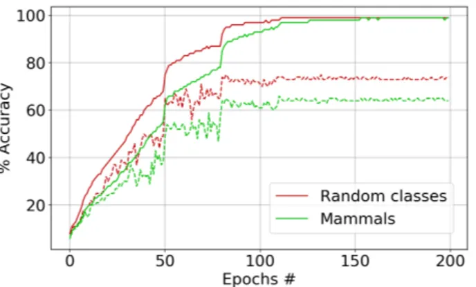
Role of class correlation: Finally, we wish to assess the role of class correlation on accuracy. Towards this goal, we fixed K = 25 classes but along with randomly sampling classes, also constructed an alternative dataset by gathering related classes. Specifically, we focused on 25 classes of mammals obtained by aggregating the following five superclasses [29]: (a) aquatic mammals, (b) small mammals, (c) medium-sized mammals, (d) large carnivores, (e) large omnivores and herbivores. Here each superclass contains five classes. In light of Lemma 3.4, which states that class correlations increases the test loss, Figure 3 compares the randomly selected classes with the mammal
Fig. 3: Comparison of 25 random classes and 25 mammal-related classes with QL. The increased class correlations slows down the optimization and reduces the test accuracy, consistent with Lemma 3.4.
classes for QL. We find that in both cases, WideResNet manages to achieve 100% training accuracy. However training with mammals dataset (rather than random classes) lead to slower training and worse test accuracy.
V. CONCLUSIONS
This work provided a theoretical and empirical comparison of cross-entropy (CE) and quadratic loss (QL). Using a mixture model, we argued that QL results in a more over-determined optimization problem and leads to a less favorable optimization landscape. To mitigate these drawbacks, we introduced CCQL which modifies QL to encourage over-parameterization by focusing on the correct class. We showed that CCQL achieves competitive accuracy in CIFAR 100 in stark contrast with QL. As future work, we intend to quantify the over-parameterization of the problem in terms of the loss function and design more advanced loss functions to better guide the training process.
VI. ACKNOWLEDGEMENTS
This work is partially supported by the NSF awards CNS-1932254 and CNS-1817216.
REFERENCES
[1] Kaiming He, Xiangyu Zhang, Shaoqing Ren, and Jian Sun, “Deep residual learning for image recognition,” in Proceedings of the IEEE conference on computer vision and pattern recognition, 2016, pp. 770– 778.
[2] Zeynep Akata, Florent Perronnin, Zaid Harchaoui, and Cordelia Schmid, “Good practice in large-scale learning for image classification,” IEEE Transactions on Pattern Analysis and Machine Intelligence, vol. 36, no. 3, pp. 507–520, 2013.
[3] Ambuj Tewari and Peter L Bartlett, “On the consistency of multiclass classification methods,” Journal of Machine Learning Research, vol. 8, no. May, pp. 1007–1025, 2007.
[4] Athanasios Papoulis and S Unnikrishna Pillai, Probability, random variables, and stochastic processes, Tata McGraw-Hill Education, 2002. [5] Herve A Bourlard and Nelson Morgan, Connectionist speech recognition: a hybrid approach, vol. 247, Springer Science & Business Media, 2012. [6] George Cybenko, “Approximation by superpositions of a sigmoidal function,” Mathematics of control, signals and systems, vol. 2, no. 4, pp. 303–314, 1989.
[7] Kurt Hornik, “Approximation capabilities of multilayer feedforward networks,” Neural networks, vol. 4, no. 2, pp. 251–257, 1991.
[8] Chiyuan Zhang, Samy Bengio, Moritz Hardt, Benjamin Recht, and Oriol Vinyals, “Understanding deep learning requires rethinking generalization,” International Conference on Learning Representations, 2016.
[9] Simon Du, Jason Lee, Haochuan Li, Liwei Wang, and Xiyu Zhai, “Gradient descent finds global minima of deep neural networks,” in Proceedings of the 36th International Conference on Machine Learning, Long Beach, California, USA, 2019, vol. 97 of Proceedings of Machine Learning Research, pp. 1675–1685, PMLR.
[10] Mikhail Belkin, Alexander Rakhlin, and Alexandre B. Tsybakov, “Does data interpolation contradict statistical optimality?,” in The 22nd International Conference on Artificial Intelligence and Statistics, AISTATS 2019, 16-18 April 2019, Naha, Okinawa, Japan, 2019, pp. 1611–1619. [11] Samet Oymak, Zalan Fabian, Mingchen Li, and Mahdi Soltanolkotabi, “Generalization guarantees for neural networks via harnessing the low-rank structure of the jacobian,” arXiv preprint arXiv:1906.05392, 2019. [12] Mikhail Belkin, Daniel Hsu, and Partha Mitra, “Overfitting or perfect fitting? risk bounds for classification and regression rules that interpolate,” 06 2018.
[13] Rob A Dunne and Norm A Campbell, “On the pairing of the softmax activation and cross-entropy penalty functions and the derivation of the softmax activation function,” in Proc. 8th Aust. Conf. on the Neural Networks, Melbourne. Citeseer, 1997, vol. 181, p. 185.
[14] Douglas M Kline and Victor L Berardi, “Revisiting squared-error and cross-entropy functions for training neural network classifiers,” Neural Computing & Applications, vol. 14, no. 4, pp. 310–318, 2005. [15] Pavel Golik, Patrick Doetsch, and Hermann Ney, “Cross-entropy vs.
squared error training: a theoretical and experimental comparison.,” in Interspeech, 2013, vol. 13, pp. 1756–1760.
[16] Anna Sergeevna Bosman, Andries Petrus Engelbrecht, and Mardé Helbig, “Visualising basins of attraction for the cross-entropy and the squared error neural network loss functions,” CoRR, vol. abs/1901.02302, 2019. [17] Anna Choromanska, Alekh Agarwal, and John Langford, “Extreme multi class classification,” in NIPS Workshop: eXtreme Classification, submitted, 2013.
[18] Ian En-Hsu Yen, Xiangru Huang, Pradeep Ravikumar, Kai Zhong, and Inderjit Dhillon, “Pd-sparse: A primal and dual sparse approach to extreme multiclass and multilabel classification,” in International Conference on Machine Learning, 2016, pp. 3069–3077.
[19] Ankit Singh Rawat, Jiecao Chen, Felix Xinnan X Yu, Ananda Theertha Suresh, and Sanjiv Kumar, “Sampled softmax with random fourier features,” in Advances in Neural Information Processing Systems 32, H. Wallach, H. Larochelle, A. Beygelzimer, F. d'Alché-Buc, E. Fox, and R. Garnett, Eds., pp. 13834–13844. Curran Associates, Inc., 2019. [20] Kaifeng Lyu and Jian Li, “Gradient descent maximizes the margin of
homogeneous neural networks,” arXiv preprint arXiv:1906.05890, 2019. [21] Ziwei Ji and Matus Telgarsky, “The implicit bias of gradient descent on nonseparable data,” in Conference on Learning Theory, COLT 2019, 25-28 June 2019, Phoenix, AZ, USA, 2019, pp. 1772–1798.
[22] Le Hou, Chen-Ping Yu, and Dimitris Samaras, “Squared earth mover’s distance-based loss for training deep neural networks,” arXiv preprint arXiv:1611.05916, 2016.
[23] Krzysztof Gajowniczek, Leszek J Chmielewski, Arkadiusz Orłowski, and Tomasz Z ˛abkowski, “Generalized entropy cost function in neural networks,” in International Conference on Artificial Neural Networks. Springer, 2017, pp. 128–136.
[24] Himanshu Kumar and PS Sastry, “Robust loss functions for learning multi-class multi-classifiers,” in 2018 IEEE International Conference on Systems, Man, and Cybernetics (SMC). IEEE, 2018, pp. 687–692.
[25] Samet Oymak and Mahdi Soltanolkotabi, “Overparameterized nonlinear learning: Gradient descent takes the shortest path?,” in International Conference on Machine Learning, 2019, pp. 4951–4960.
[26] Difan Zou, Yuan Cao, Dongruo Zhou, and Quanquan Gu, “Stochastic gradient descent optimizes over-parameterized deep relu networks,” arXiv preprint arXiv:1811.08888, 2018.
[27] Roman Vershynin, “Introduction to the non-asymptotic analysis of random matrices,” in Compressed Sensing, pp. 210–268. 2012. [28] Sergey Zagoruyko and Nikos Komodakis, “Wide residual networks,” in
Proceedings of the British Machine Vision Conference (BMVC), Edwin R. Hancock Richard C. Wilson and William A. P. Smith, Eds. September 2016, pp. 87.1–87.12, BMVA Press.
[29] Alex Krizhevsky, Ilya Sutskever, and Geoffrey E Hinton, “Imagenet classification with deep convolutional neural networks,” in Advances in neural information processing systems, 2012, pp. 1097–1105.