i
A CHAOTIC APPROACH IN ANALYZING
THE ISE-100 INDEX
RABİA ÖZKAYA
107621021
İSTANBUL BİLGİ UNIVERSITY
INSTITUTE OF SOCIAL SCIENCES
FINANCIAL ECONOMICS
SUPERVISOR
KORAY AKAY
iii
Acknowledgements
I would like to express my gratitude to my thesis supervisor Assistant Professor Koray AKAY for his guidance and contribution. I feel indebted to him for his generosity in sharing his time, contiuned support and patience. And I would like to thank to Director of The Master of Science in Financial Economics Program Orhan ERDEM and Ege YAZGAN.
I am deeply thankful to Ata OZKAYA who supported me for this study, who shared his time and ideas to improve the study with comments and contributions. Last but certainly not least, I want to thank my family my father Mehmet ÖZKAYA and my mother Gönül ÖZKAYA for their enthusiastic and unending support during my master education.
iv
Abstract
This study aims to discuss the validity of the Efficient-Market Hypothesis by investigating the time evolution characteristics of ISE-100 index. Two major analysis methods are used and compared. First, the nonlinear dynamical behavior of the daily-return values of ISE-100 index (01.1990-10.2009) is explored by implementing Chaos Theory and applying recent chaotic analysis methods. Second, the same data set is used for linear time series modelling and by applying unit root tests we explore the stochastic behavior of the series. Finally, the comparison of the two major analysis is introduced. Our results uncover the chaotic behavior of the ISE-100 index and thus give more room to the predictivity analysis of daily-return values.
Keywords: Efficient-Market Hypothesis, Nonlinear Dynamical Analysis, Wolf’s
Algorithm, Kantz’s Algorithm, Lyapunov Exponent, Chaotic Behavior, ARIMA, Nonstationarity Analysis.
v
Özet
Bu çalışma, IMKB-100 endeksinin zaman içindeki değişiminin efficient market hipotezindeki geçerliliğinin tartışmasını hedefler. İki analiz metodu uygulanmış ve karşılaştırılmıştır. İlk olarak, IMKB-100 endeksinin kapanış değerleri getirilerinin (01.1990-10.2009) doğrusal olmayan dinamik davranışını kaos teorisi uygulayarak araştırıp, halen kullanılmakta olan kaotik analiz metotları kullanarak testler yapılması oluşturmuş, ikincil olarak, aynı data setine unit root testi uygulayarak, stokastik davranışını araştırmak için doğrusal zaman serisi analiz metodu uygulanmıştır.
Son olarak iki analizin kıyaslaması yapılmış, sonuçlarımızın IMKB-100 endeksinin kaotik davranışını ortaya çıkarması ile, günlük kapanış değerleri getirilerinin tahmin edilebilirliğine daha fazla olanak sağladığı görülmüştür.
vi
Table of Contents
1. Introduction……….1
2. Review of The Literature……...………...4
3. Preliminary Notions………..10
3.1. Defining an Attractor ………...11
3.1.1. Chaotic Attractor………...11
3.1.2. Constructing a Phase Space………...13
3.1.3. The Fractal Dimension………...14
3.1.3.1. Recurrence Plot………..15
3.1.4. Characteristic Exponent (Lyapunov Exponent)……18
3.1.4.1. Sensitive Dependence on Initial Conditions………..19
4. Methodology……….21
4.1. Introducing the Nonlinear Dynamical System………..24
4.2. Computing Lyapunov Exponents………..30
4.2.1. Wolf’s Algorithm………..30
4.2.2. Gencay and Dechert’s Algorithm………..31
vii
4.2.4. The Comparison of the Effectiveness of Wolf’s, Gencay Dechert’s and Kantz’s
Algorithms………37
5. Time Series Analysis of ISE -100 Composite Index……….40
5.1. Time Series Analysis……….41
5.1.1. Unit Root and Integrated Processes………..42
5.1.1.1.
Unit Root Analysis……….45
5.1.1.2. Application of Time Series Modelling Worldwide Stock Exchanges (SE)………46
5.2. Application of Time Series Modelling to ISE-100 Stock Exchange………...47
5.2.1. Results of The Analysis………...…...48
5.3. Comparison Between ARIMA Modelling and Chaos Modelling of ISE-100………....52
6. Results of Chaotic Analysis………..53
6.1. Implications ………..55 6.2. Practical Considerations……….55 6.3. Final Considerations ………..56 7. Conclusion ……….. 56 8. References………....…58 Appendix………..…65
viii
List of Tables
Table Page
1 Related Researches………4
2 Some Properties of Stationary and Integrated Process……….45
3 Results of the ADF Test statistics of
1 log t t y y Residuals……….50
4 Correlation Matrix of Index Serie……….50
5 Average Log Distance of daily reel-return values………53
6 The Average Distances in Phase Space of daily reel-return values.54
7 Average Distances in Phase Space of daily reel-return values with Tho max 35………...……54
ix
List of Figures and Graphics
Figure Page
1 Statistical Properties of logarithmic return ISE-100……….……..40
2 Time Plot of y Residuals……….……..….49 t
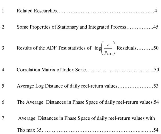
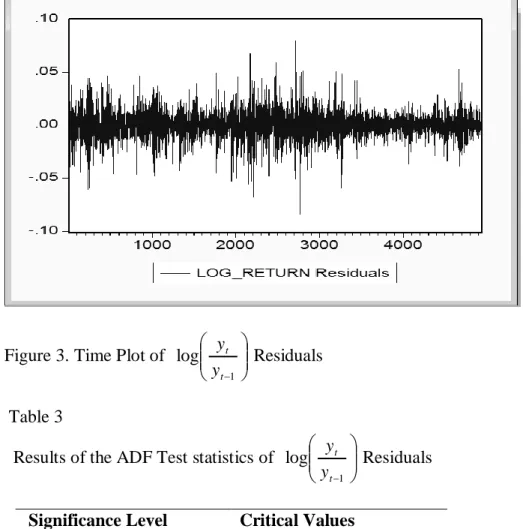
3 Time Plot of 1 log t t y y Residuals….………..50 4 Time Plot of 1 log t t y y ………..51 Graphics
A1 Recurrence Plot Analysis of deflated values of ISE-100 Period Between 01.90- 01.98 ,[1-2000]………..65
A2 Recurrence Plot Analysis of deflated values of ISE-100 Period Between 94Q1-95Q1 and 94 Crisis ...………65
A3 Recurrence Plot Analysis of deflated values of ISE-100 Period Between 98Q1- 99Q2 and 98 …..………..66
A4 Recurrence Plot Analysis of deflated values of ISE-100 Period Between 2000.06 -2002Q1 and 2001 ……….66
B1 Recurrence Plot Analysis of nominal closing values of ISE-100 Period Between Data: 08.93- 01.95……….67
x
B2 Recurrence Plot Analysis of nominal closing values of ISE-100 Period Between Data: 08.97 - 02.99 the points [1900-2270]……..67
B3 Recurrence Plot Analysis of nominal closing values of ISE-100 Period Between Data : 10.2000 - 07.2001 the points [2669-2900]………..…68 B4 Recurrence Plot Analysis of nominal closing values of ISE-100
Period Between Data 01.2003- 02.2006………..……68 B5 Recurrence Plot Analysis of nominal closing values of ISE-100
Period Between Data 03.95- 08.97 between two crisis………69 B6 Recurrence Plot Analysis of nominal closing values of ISE-100
Period Between Data: 99Q1-10.2000 between two crisis…………69 C1 Recurrence Plot Analysis of reel return of ISE-100 Period Between
1000- 1350………..……….70 C2 Recurrence Plot Analysis of reel return of ISE-100 Period Between
1900-2300………...………..70 C3 Recurrence Plot Analysis of reel return of ISE-100 Period Between
1
1. Introduction
Until relatively recently, it was more or less taken for granted that movements in stock market prices were over-whelming stochastic in nature, if not actually a random walk. The assertion seemed unchallengeable on theoretical grounds- namely, consistency with the ruling efficient-market paradigm or efficient-market hypothesis (EMP). The EMP basically says that current prices fully reflect all known information. This implies that there is little or no correlation between returns; price changes occur in a random fashion, in reaction to new information and price movements do not follow any patterns or trends. That is, past price movements cannot be used to predict the future price movements but follow what is known as a random walk, an intrinsically unpredictable pattern (Campbell et al., 1997; Fama, 1965). This assumption-which has never been conclusively proven-is the bed-rock upon which standard statistical analysis of the markets has been built. The law of large numbers, for example, applies only if price changes are independent (i.e., "efficient"). And it is the law of large numbers that validates statistical calculus and other linear models. Under the EMP, stock return process should be random. Therefore, it seems improbable a priori that the pattern of returns could be explained to any substantial degree by a deterministic process, given that the major cause of market movements is normally assumed to be the random flow of information. The mathematical expression of EMP is that the financial time series is characterized by a linear model and is independent and identically distributed (i.i.d.), so behave in a random manner. According to these implications, the importance of this research theme comes from the fact that chaos and EMP . As regards to the debate on the behavior of stock-index data and EMP, in this study we address two important questions that have been the focus of a substantial and still growing literature in recent years and that have been analyzed for many other stock-indexes of developed countries. Is there nonlinear dependence in ISE-100 stock-market returns (or closing values)? And, if so, is the nonlinear structure characterized by low-dimensional chaos? In other
2
words, is the apparent randomness of the time series pattern of returns explicable, in part at least, by a deterministic process?
2. Review of The Literature
Up to 90’s, many economic studies examined U.S, U.K and Canadian markets (Kendall, 1953; Brealey, 1970; Dryden, 1970; Cunningham, 1973; Brock, 1987) and support the EMP. The studies on the United Kingdom stock market report the weak form market efficiency as conjectured by the pioneering study Fama (1965) – namely, that the linear modeling techniques have limitations as they are not sophisticated enough to capture complicated “patterns” which chartists claim to see in stock prices. In fact, linear models will prove successful only to the extent that the system being analyzed is itself linear.
If the system is nonlinear, the models will work, at best, only under "ideal" conditions and over short time periods. Thus the application of linear models to the market may be questionable, in view of recent research suggesting that the capital markets, and the economy as a whole, may be governed in part by non-linear dynamics. The main reason is briefly: when nonlinear dynamics are involved, a deterministic system can generate “random-looking” results that nevertheless exhibit persistent trends, cycles (both periodic and non-periodic) and long-term correlations.
At last in 90’s, several developments that have led to serious questioning of the proposition that stock returns are inherently unpredictable have taken place. First, researchers using conventional econometric methods have uncovered several deviations from efficiency in the behavior of stock prices (Fama 1991). Second, the correlated studies in physics (Grassberger and Procaccia 1983; Wolf et al., 1985; Nychka et al., 1992; Gencay and Dechert 1992; Rosenstein et al.,1993; Kantz 1994), thermo dynamical engineering (Takens 1981; Ott E 1993), biomedical engineering (Barlow 1985; Schuster 1989; Basar 1990; Jansen 1991), and hydrodynamics (Eckamnn 1983; Eckamnn et al., 1987) have resulted in the discovery of
3
“random-looking or apparently random” behaviors running the dynamical systems. Moreover, the studies in physics mentioned above also involved in the development of several tests capable of detecting nonlinear as well as linear patterns in the observed data. Third, the exciting progress in the last 30 years in understanding the nonlinear dynamical systems means that we can now entertain the possibility of certain types of deterministic process in financial data (Peters 1991; Lorenz, 1993; Pesaran and Potter, 1993; Creedy and Martin, 1994; Trippe, 1995; Abhyankar et al., 1997; Hinich and Rothman, 1998; Mantegna and Stanley 2000; McKenzie, 2001; Barnett and William, 2004; Muckley, 2004; Das and Das, 2007; Hagtvedt 2009). In particular, it has become clear that many low-dimensional deterministic nonlinear systems are capable of generating output that is in most respects indistinguishable from white noise.
It is important to note that, as far as financial series are concerned, this type of process could be consistent with market efficiency if it is only forecastable at horizons too short to allow any trade-off by speculators. The unresolved issue addressed in Scheinkman and LeBaron (1989), Peters (1991), Abhyankar et al., (1997), Mandelbrot (1999) relates, therefore, to whether stock-market index returns1 are best represented by a purely stochastic process or rather by a nonlinear deterministic structure. As can be seen from Table 12, there is already a substantial literature examining the questions addressed in these studies. Most of the financial research so far has concentrated on stock-market indexes, though a few have looked elsewhere (future markets, gold, and silver prices, energy prices, monetary movements, interest rates).
All of these studies address the nonlinear deterministic structure3 (static and dynamic) of a dynamical system which is assumed to generate
1
Following the findings of Fama and French (1992), Hagtvedt (2009) use the dynamic characteristics of individual stocks rather than stock-index to examine anomalies in Sharpe’s Capital Asset Pricing Model (CAPM) (Sharpe 1964)
2
To conserve space, we state the studies which are mainly concerned with stock-indexes. The related studies on other types of financial data are cited in the text.
3
4
the observed time series data and which is mainly detected by applying various tests (Ott E, 1993; Kantz and Schreiber, 1997). These tests are Brock-Dechert-Scheinkman (BDS) test for independence, estimation of the correlation dimension (CD) (Grassberger and Procaccia 1983a) for quantitative description of complexity in terms of the number of degrees of freedom and Kolmogorov entropy (Grassberger and Procaccia 1983b) estimate the degree of order-disorder and thus of the complexity of a dynamic system. Finally, if nonlinear structure is observed4, then Lyapunov Exponent (LE) should be obtained by one of the “appropriate” algorithms (Wolf et al., 1985; Nychka et al., 1992; Gencay and Dechert 1992; Rosenstein 1993; Kantz 1994).
As it can be seen from Table 1, the most commonly deployed test is Brock-Dechert-Scheinkman (BDS) test for independence, though several authors have relied on estimates of the correlation dimension (CD) and Kolmogorov Entropy estimation. While some of the authors who detect nonlinearity in observed time series data estimate LE’s, some others find it sufficient to show the nonlinearity and do not estimate LE’s.
Table 1
Related Researches
Authors Dataset Sample
Info Tests Results Abhyankar et al., (1997) The S&P 500, the DAX, the Nikkei 225, and the FTSE-100 S=10000 1) BDS 2) Nychka et al.,LE test 1) Nonlinear 2) No evidence of Chaos 4
According to Gencay and Dechert (1992), if one of the Lyapunov Exponents is positive, then the system is nonlinear. Therefore, we do not in fact apply nonliearty test before examining chaotic behavior.
5 Abhyankar et al., (1995) FTSE-100 cash S=60000 1) Bispectral linearty test 2) BDS 3) LE 1) Nonlinear 2) No evidence of Chaos Eldridge and Coleman (1993) FTSE-100 cash and futures S=1000 6.1984-9.1987 1) Correlation Dimension test 2) Wolf’s LE
Not i.i.d and consistent with chaos Hsieh (1993) Foreign Currency spots and futures S=1275, daily 2.1985-3.1990 Tests of linear and nonlinear predictabilitie s No linear and nonlinear predictables Philippatos et al.,(1993) Ten major national stock indexes S=833, weekly levels and returns 1.1976-12.1991 BDS test Nonlinear Van Quang T (2006) Czech stock index PX50 S=2270, daily returns 1.1997-9.2005 1) BDS test 2) LE 1) Nonlinear 2) Evidence of chaos Vaidyanatha n and Krehbiel (1992) S&P500 future mispricing S=1500 1) BDS test 2)Correlation Dimension test Nonlinear and low-dimensional chaos Vassilicos et al., (1992) NYSE S=30000 1) Wolf’s LE 2)Correlation Dimension test No evidence of chaos
6 Brock et al.,(1991) (1)CRSP (2) S&P 500 S=2510 daily 1.1974-12.1983 1)BDS 2)Dimension plots Nonlinearty ; little evidence of nonlinear forecastability Kodres and Papeil (1991) British P, Canadian D, DM, JYEN, Swiss Franc S=3500 daily futures 7.1973-3.1987 BDS test Nonlinear Frank and Stengos (1990) Returns of (1)Gold (2) Silver prices (1)S=2900 (2) S=3100 1) Corr. Dim. Test 2)Kolmogoro v Entropy 1)dimension of 6 2)positive;low -dimensional chaos Mayfield and Mizrach (1989) S&P 500 S=20000, 20 seconds, 1987-1989 Correlation dimension tests Low-dimensional chaos Scheinkman and LeBaron (1989) CRSP weighted index S=5200, daily returns BDS test on original and filtered data Evidence of nonlinearty Panas and Ninni (2000) Rotterdam and Mediterranea n petroleum markets (1) oil products S=1161 daily, 1.1994-8.1998 1) Correlation dimension test 2) BDS test 3)Kolmogoro v entropy 4) Wolf’s LE test Evidence of Chaos Vraon and Jalilvand (1994) TSE-300 index S=3000 and 2500; daily and monthly 1.1977-12.1991 1) Correlation dimension test 2) BDS test 1) Evidence of chaos in monthly data 2)little evidence of chaos in daily returns
7 Serletis and Dormaar (1996) Australlian Dollar and USD exchange rates S=300, weekly 1.1987-6.1993 1) Nychka et al. nonparametri c LE test 1)Evidence of Chaos Matilla-Garcia M (2007) Energy futures (1)Natural gas (2) unleaded gas (3) light crude oil New York Mercantile Exchange (NYMEX) daily, S: 3700 3.1990-10.2005 1) BDS test 2) Wolf’s LE test 3) Rosenstein LE test 1)Nonlinearit y in future returns 2)Evidence of Chaos Krager and Kugler (1992) Exchange rates JYEN; DM; FF; Italian Lira; Swiss Franc S=500 weekly returns 6.1980-12.1990 BDS test Nonlinear EE Peters (1991) S&P 500 index Snot indicated 1)CD 2)Wolf’s LE 1)Nonlinearit y 2) Evidence of chaos E.Panas (2002) London Metal Exchange Market S=2987dail y closing metal prices 1.1989 to 12.2000 1) Correlation Dimension test 2) LE 1) The metal commodities zinc and tin are chaotic. Atin Das, Pritha Das (2007) Foreign Exchange Rate of Twelve countries S=8500 daily 01.1971-12.2005 1)Wolf’s LE test 1) Nonlinearity 2) Evidence of chaos M.Neugart (1999) German labour market S not indicated. 1) Correlation dimension test 2) BDS test 1) Chaos does not occur.
8
Following Table 1 and as regards the main conclusions of the literature, there is a broad consensus of support for the proposition that the return ( or closing values) process is characterized by a pattern of nonlinear dependence. In particular, BDS test almost invariably reject the null of i.i.d process. On the other hand, the evidence on chaos is more mixed, with some evidence of low-dimensional structure in the U.S. stock-market index (Mayfield and Mizrach 1989; Vaidyanathan and Krehbiel 1992). Note, however, that these conclusions are based on CD, rather than LE estimates. Peters (1991) examine the S&P 500 by calculating CD and by estimating the largest LE as proposed by Wolf et al. (1985).
The author reports strong evidence of chaos in S&P 500 index. Moreover, for four well-known stock-index including S&P 500 index (the S&P 500; the DAX; the Nikkei 225; the FTSE-100) are analyzed by Abhyankar et al., (1997) and the authors estimate largest LE by using the method Wolf et al., (1985) and Nychka et al.,(1992). Even though Abhyankar et al., (1997) find the presence of nonlinear dependence in the returns on all indexes; the authors report no evidence of low-dimensional chaos and conclude that the data are dominated by a stochastic component. Findings of Abhyankar et al. (1997) are also consistent with the results of Scheinkman and LeBaron (1989) in sense of nonlinearity. Scheinkman and LeBaron (1989) report the existence of the nonlinearity for U.S weekly returns on the Center for Research in Security Prices (CRSP) value-weighted index, employing the BDS statistic, and find rather strong evidence of nonlinearity and some evidence of chaos. These evidences from different authors are sufficient to call into question the EMP, which underlies the linear modelling used in most capital market theory. It also lends validity to a number of investment strategies that should not work if markets are efficient, including trend analysis, market timing, value investing and tactical asset allocation. This finding is of particular importance for practitioners, because experience has shown that these strategies do work when properly applied, even though theory tells us they should not work in a random-walk environment. Conversely, strategies that depend upon efficient markets and continuous
9
pricing, such as portfolio insurance, Alexander filters and stop/loss orders, become suspect, because chaotic markets are neither efficient nor continuously priced. This calls into question the Capital Asset Pricing Model (CAPM) and most option-pricing theories, which are based upon normal distributions and finite variances. It is worthwhile to note that, by focusing on the chaotic properties of stocks at the firm level rather than the properties of indices, Hagtvedt (2009) obtains dominant LE and the CD for weekly returns to individual stocks and concludes that the firm characteristics size (market value) was found to exhibit chaotic characteristics of the stocks showing the anomalies in Sharpe’s Capital Asset Pricing Model (Sharpe 1964). For other well-know world indexes, there are also several studies. Sewell et al. (1993) report evidence of dependency in the market index series in Japan, Hong Kong, South Korea, Singapore and Taiwan. De Lima (1995) argues that for the U.S data, nonlinear dependence is present in stock returns after the 1987 crash. Small and Tse (2003) analyze daily returns from three financial indicators: the Dow Jones Industrial Average, the London gold fixings, and the USD-JPY exchange rate and the authors conclude that all three time series are distinct from linear noise or conditional heteroskedastic models and that there therefore exists detectable deterministic nonlinearity that can potentially be exploited for prediction.
Despite the affirmative chaos test results, there are some critiques of the chaos in the literature as well (Lee et al., 1993). Hamill and Opong (1997) conclude that even though there is nonlinear dependence in Irish stock returns, there is no evidence of chaos. Willey (1992) find no evidence of chaos in the Financial Times Industrial Index.
Apart from stock-index analysis, Barnett et al. (1996) report the successful detection of chaos in the US division monetary aggregates. This conclusion is further confirmed by several authors (e.g. Hinich and Rothman 1998; Barnett and William, 2004). Frank and Stengos (1989) obtain similar results by investigating daily prices for gold and silver, using the correlation dimension and the Kolmogorov entropy. Serletis and Gogas
10
(1997) find the evidence consistent with a chaotic nonlinear generation process in seven East European black market exchange rates. Furthermore, foreign exchange markets are an essential domain in which chaos has been detected (Mantegna and Stanley, 2000; Das and Das, 2007). Many researchers (e.g. Granger and Newbold, 1974; Campbell et al., 1997; Lee et al., 1993; Bonilla et al., 2006) argue that financial market series exhibit nonlinearity. The terms of many financial contracts such as options and other derivative securities are also nonlinear (Mantegna and Stanley, 2000).
By examining the unemployment and the rate of change of money wage rates in the U.K. 1861-1957 Fanti and Manfredi (2007) detect chaotic behavior in wage and unemployment rates.
The studies on ISE-100 index are relatively less in number. Some studies on Turkish ISE market (e.g. Bayramoglu, 2007; Ozgen, 2007) demonstrate that the market is not efficient. Moreover, most of the studies on the behavior of ISE market prices supported the weak form market efficiency against the existence of chaos (Kenkül, 2006; Topçuoglu, 2006; Çıtak, 2003; Adali, 2006). On the other hand, in contrast with the above studies on ISE-100, by applying BDS, Hinich Bispectral, Lyapunov Exponent and NEGM tests Ozer (2010) reject the efficient market hypothesis that the ISE-100 all share equity index series is random, independent and identically distributed (i.i.d).
3. Preliminary Notions
3.1. Defining An Attractor
An attractor is a state that defines equilibrium for a specific system. As we shall see, equilibrium does not necessarily mean a static state, as econometric models define the term.
A simple attractor is a point attractor. A pendulum with friction is an example of a point attractor.
11
If you were to plot the velocity of the pendulum versus its position, you would obtain a graph that spirals in towards the origin, where velocity and position are zero. At this point, the pendulum has stopped.
A graph of velocity versus position is an example of the phase space of a system. Each point on the graph defines the state of the system at that time. All paths in phase space lead to a point attractor, if one exists. No matter where the motion in phase space initiates, it must end up at the origin-the point attractor. A pendulum that periodically receives energy goes back and forth with no variation in its path. Its phase-space plot becomes a closed circle, with the origin at its center. This is called a limit cycle attractor. The radius of the circle is determined by the amplitude of the pendulum's swing. As a time series, a limit cycle appears as a simple sine wave.
3.1.1. Chaotic Attractor
A third kind of attractor is a chaotic, or fractal, attractor. With a chaotic attractor, the trajectories plotted in phase space never intersect, although they wander around the same area of phase space. Orbits are always different, but remain within the same area; they are attracted to a space, but never converge to a specific point. Cycles, while they exist, are non-periodic. With a chaotic attractor, equilibrium applies to a region, rather than a particular point or orbit; equilibrium becomes dynamic. For example in economics, equilibrium is commonly defined as static. In other words, an economic system is commonly thought to tend to equilibrium (a point attractor) or to vary around equilibrium in a periodic fashion (a limit cycle). But there is no evidence that capital markets tend toward either type of equilibrium. If anything, the actual behavior of economic time series appears to be non-periodic. That is, they have cycles without well defined periods. If the markets are non-periodic, then limit cycles and point attractors cannot define their dynamics. Chaotic Attractors using a simple convection model, Edward Lorenz (1963) was able to define the first known chaotic attractor. The model is based on a fluid heated from below.
12
At low temperature levels, heat transfer occurs by convection; the water molecules behave independently of one another. As the heat is turned up, a convection roll starts; the water molecules behave coherently, and the warmer fluid on the bottom rises, cools as it reaches the top and falls back to the bottom. The water molecules trace a limit cycle. If the heat is turned up further, turbulence sets in; the fluid churns chaotically. At this point, the water's phase space becomes a chaotic attractor.
Chaotic attractors have an interesting property. Because of the possible nonlinearities in the underlying system, any errors in measuring current conditions eventually overwhelm any forecasting ability, even if the equations of motion are known. In other words, our ability to predict the future of a chaotic system is limited by our knowledge of current conditions. Errors in measurement grow exponentially in time, making any long-term forecast useless. This sensitive dependence on initial conditions made Lorenz conclude that any attempts at weather forecasting beyond a few days were doomed. If the economic cycle is governed by a chaotic attractor, it is easy to see why long-term econometric forecasts during the '70s and '80s were flawed.
How do we determine if a system has an underlying chaotic attractor? First, a phase space for the system must be constructed. (When the equations of motion are not known, this is not a simple task.) The resulting phase space must meet two criteria for a chaotic attractor:
(1) a fractal dimension
(2) sensitive dependence on initial conditions.
In the physics and engineering, various techniques have been developed to measure these items using experimental data.
If this attractor arises, this is because the relations between the variables that govern market movements are nonlinear. Nonlinear systems are characterized by trends and long-term correlations. If the market is
13
nonlinear, then the widespread use of standard statistical analysis is questionable. In particular, the Efficient Market Hypothesis and the Capital Asset Pricing Model (in its current form) are suspect as workable theories.
3.1.2. Constructing a Phase Space
A phase space consists of "m" dimensions, where each dimension is a variable involved in defining the time evolution (“motion”) of the system. In a system where the equations of motion are known, constructing a phase space is simple. However, we rarely know the dynamics of the real system generating the observed time series data. By plotting one variable with different lags, one can reconstruct the original, unknown phase space with one dynamic, observable variable. This reconstructed phase space has all the characteristics of the real phase space, provided the lag time and embedding dimension are properly specified. (We discuss below how these parameters are determined.) Now the question becomes, what do we use as our single observable variable? Traditional analyses of the stock market use the percentage change in price (returns) or a logarithmic first difference. This removes the autocorrelations inherent in the original price series and makes the series suitable for linear statistical analysis. However, what standard statistical analysis considers undesirable may in fact be evidence of a nonlinear dynamic system. That is, the use of percentage changes in price may destroy any delicate nonlinear structure present in the data. In constructing attractors such as the Lorenz attractor, scientists use the actual value of the variables, not the rate of change. We apply this approach to our study of financial data. Economics, however, presents a problem that the physical sciences do not. As the economy grows, stock prices grow. Stock price data thus have to be detrended; in order to study the motion of stock prices, economic growth must be filtered out. Ping Chen, in his study of monetary aggregates, filtered out the internal rate of growth over the period.
This method has the appeal of simplicity, but it assumes a constant rate of growth, which is unrealistic. As we know, economic growth is not constant, but varies over time.
14
Therefore we use the deflated ISE-100 time series as our dynamic observable. From this series, we can reconstruct a phase space to obtain a fractal dimension and to measure sensitive dependence on initial conditions.
3.1.3. The Fractal Dimension
The fractal dimension of phase space gives us important information about the underlying attractor. More precisely, the next-higher integer above the fractal dimension is the minimum number of variables we need to model the dynamics of the system. This gives us a lower bound on the number of degrees of freedom in the whole system. It does not tell us what these variables are, but it can tell us something about the system's complexity. A low dimensional attractor of, say, three or four would suggest that the problem is solvable. A pure random process, such as white noise, fills whatever space it is plotted in (Recurrence Plot, Eckmann 1987). In two dimensions it fills the plane. In three dimensions, it fills the three-dimensional space, and so on for higher dimensions. In fact, white noise assumes the dimension of whatever space you place it in because its elements are uncorrelated and independent. The fractal dimension measures how an attractor fills its space. For a chaotic attractor, the dimension is fractional; that is, it is not an integer. Because a chaotic attractor is deterministic, not every point in its phase space is equally likely, as it is with white noise.
Grassberger and Procaccia (1983a) estimate the fractal dimension as the correlation dimension, D. D measures how densely the attractor fills its phase space by finding the probability that any one point will be a certain distance, R, from another point.
The correlation integral, Cm(R), is the number of pairs of points in an m-dimensional phase space whose distances are less than R.
For a chaotic attractor Cm increases at a rate R . This gives the following D
relation D
R
15
By calculating the correlation integral, Cm, for various embedding dimensions, m, we can estimate D as the slope of a log/log plot of Cm and R. Grassberger and Procaccia have shown that, as m is increased, D will eventually converge to its true value. Assume that for a dynamical systemD2,4. This means that the dynamics of this particular system can be defined with a minimum of three dynamic variables. Once these variables are defined, we can model the system. Of course, the fractal dimension does not tell us what the variables are, but only how many variables we need, at a minimum, to construct the model. Our estimate is low enough to suggest that the problem is solvable.
3.1.3.1. Recurrence Plot
The method of recurrence plots (RP) was firstly introduced by Eckmannn et al., (1987) to visualize the time dependent behavior of the dynamics of systems ( the recurrence of states in a phase space) which can be pictured as a trajectory in the m-dimensional phase space. It represents the recurrence of the phase space trajectory to a certain state, which is a fundamental property of deterministic dynamical systems. The main step of this visualization is the calculation of the distances between all points lying in the phase-space. Usually, a phase space does not have a low enough dimension (two or three) to be pictured. Higher-dimensional phase spaces can only be visualized by projection into the two or three-dimensional sub-spaces. However, Eckmann's tool enables us to investigate the
m-dimensional phase space trajectory through a two-dimensional
representation of its recurrences. Such recurrence of a state at time i and a different time j is pictured within a two-dimensional squared matrix with black and white (and grey) dots, where black dots mark a recurrence, and both axes are time (number of observed data) axes. The recurrence plot exhibits characteristic large-scale and small-scale patterns which are caused by typical dynamical behavior, e. g. diagonals (similar local evolution of different parts of the trajectory) or horizontal and vertical black lines (state does not change for some time). The RP exhibits characteristics which can
16
be observed as both large scale and small scale patterns). The first patterns (large scales) were denoted by Eckmann et al. (1987) as typology and the latter (small scales) as texture. The typology offers a global impression which can be characterized as homogeneous, periodic, drift and disrupted.
Homogeneous RPs are typical of stationary and autonomous systems
in which relaxation times are short in comparison with the time spanned by the RP. An example of such an RP is that of a random time series.
Oscillating systems have RPs with diagonal oriented, periodic recurrent structures (diagonal lines, checkerboard structures). For
quasi-periodic systems, the distances between the diagonal lines are
different. However, even for those oscillating systems whose oscillations are not easily recognizable, the RPs can be used in order to find their oscillations.
The drift is caused by systems with slowly varying parameters. Such slow (adiabatic) change brightens the RP's upper-left and lower-right corners.
Abrupt changes in the dynamics as well as extreme events cause
white areas or bands in the RP. RPs offer an easy possibility to find
and to assess extreme and rare events by using the frequency of their recurrences.
17
In the figure above, the upper series are the original observed time series and lower series are Recurrence Plots associated to them, respectively.
1. White Noise 2. Sine Wave 3. Lorenz System with linear time trend 4. Distrupted (Brownian motion) with rare shocks.
In addition to the large scales defined above, the closer inspection of the RPs reveals small scale structures (the texture) which are single dots, diagonal lines as well as vertical and horizontal lines ( the combination of vertical and horizontal lines obviously forms rectangular clusters of recurrence points).
1. Single, isolated recurrence points can occur if states are rare, if they do not persist for any time or if they fluctuate heavily.
2. Certain points in the observed time series are parallel to each other i.e. they have same values but are placed at a different interval. A diagonal line occurs when a segment of the trajectory runs parallel to another segment, i.e. the trajectory visits the same region of the phase-space at different times. The length of this diagonal line is determined by the duration of such similar local evolution of the trajectory segments. The direction of these diagonal structures can differ. These stretches can be visualized as diagonal lines in the recurrence matrix.
These diagonal lines are called deterministic, because they represent a deterministic pattern in the series (the deterministic local evolution of states in the series). Therefore, Lyapunov exponent is defined as inverse of the length of these diagonal patterns.
a.) Diagonal lines parallel to main diagonal line represent the parallel running of the trajectories for the same time evolution.
b.) Diagonal lines perpendicular to main diagonal line represent the parallel running with contrary times ( may show improper embedding)
3. A vertical (horizontal) line marks a time length in which a state does not change or changes very slowly. It seems that the state is trapped for
18
some time. This is a typical behavior of laminar states (intermittency) and widely used in fluid dynamics in order to model the flow of a river when its debit forced to narrow.
3.1.4. Characteristic Exponent (Lyapunov
Exponent)
Lyapunov exponents, which provide a qualitative and quantitative characterization of dynamical behavior, are related to the exponentially fast divergence or convergence of nearby orbits in phase space. A system with one or more positive Lyapunov exponents is defined to be chaotic. To measure LE, we monitor the long-term growth rate of small volume elements in an attractor.
Each positive exponent reflects a "direction" in which the system experiences the repeated stretching and folding that decorrelates nearby states on the attractor. Therefore, the long-term behavior of an initial condition that is specified with any uncertainty cannot be predicted; this is chaos. An attractor for a dissipative system with one or more positive Lyapunov exponents is said to be "strange" or "chaotic"
The magnitudes of the Lyapunov exponents quantify an attractor's dynamics in information theoretic terms.
The exponents measure the rate at which system processes create or destroy information ; thus the exponents are expressed in bits of information/s or bits/orbit for a continuous system and bits/iteration for a discrete system. For example (Wolf et al., 1985), in the Lorenz attractor the positive exponent has a magnitude of 2.16 bits/s . Hence if an initial point were specified with an accuracy of one part per million (20 bits), the future behavior could not be predicted after about 9 s [20 bits/(2.16 bits/s)], corresponding to about 20 orbits. After this time the small initial uncertainty will essentially cover the entire attractor, reflecting 20 bits of new information that can be gained from an additional measurement of the system.
19
3.1.4.1. Sensitive Dependence on Initial Conditions
The positive maximal Lyapunov exponent implies the sensitive dependence of the dynamical system on initial conditions. Chaotic attractors are characterized by sensitive dependence on initial conditions. An error in measuring initial conditions will grow exponentially, so that a small error could dramatically affect forecasting ability. The further out in time we look the less certain we are about the validity of our forecasts. Contrast this with the linear models used in econometric forecasts. A small change in measuring current conditions has little impact on the results of a forecast. Theoretically, linear models imply that, if we have enough variables, we can forecast an indefinite period into the future. While the certainty of linear models is desirable, the uncertainty inherent in non-linear dynamics is closer to practical experience.
Lyapunov exponents measure the loss in predictive power experienced by non-linear models over time. Lyapunov exponents measure how nearby trajectories in phase space diverge over time. Each dimension in phase space has its own Lyapunov exponent. A positive exponent measures expansion in phase space. A negative one measures contraction in phase space. For a fixed point in three dimensions, the Lyapunov exponents are negative. For a limit cycle, two exponents are negative and one equals zero. For a chaotic attractor, one is positive, one negative and one zero. A chaotic attractor is characterized by the largest Lyapunov exponent being greater than zero. It represents the divergence of points in phase space, or the sensitive dependence on the conditions represented by each point. When the equations or motion are known, Lyapunov exponents can be calculated by measuring the divergence of nearby orbits in phase space. In a linear world, points that are close together in phase space would remain close together; this reflects the linear world, where a small error in measurement has little effect on the result. In a non-linear world, things are different. Nearby points will diverge as the differences in initial conditions compound.
20
This method involves measuring the divergence of nearby points in the reconstructed phase space over fixed intervals of time. First, we choose two points that are at least one mean orbital period apart. The distance between the two points is measured after the fixed evolution period. If the distance is too long, one of the points is replaced. (This is necessary to ensure that we measure only the expansion of the points in phase space; if the points are too far apart, they will fold into one another.) In addition, the angle between the points is measured to keep the orientation of the points in phase space as close as possible to the original set.
In theory, with an infinite amount of noise-free data, there occurs no difficulty. However, the real world presents us with a finite amount of noisy data. This means that the embedding dimension, m, the time lag, t, and the maximum and minimum allowable distance must be chosen with care. Wolf et al. give a number of "rules of thumb" for dealing with experimental data. First, the embedding dimension should be larger than the phase space of the underlying attractor. The time lag used to reconstruct the phase space must be computed; the maximum length of growth should be no greater than 10 per cent of the length of the attractor in phase space. Finally, the evolution time should be long enough to determine stretching without including folds. However, these rules of thumb are more evaluated in recent years (Kantz and Schreiber 1997).
Once done, the calculation over a long time series should converge to a stable value of LE. If stable convergence does not occur, it is possible that the parameters have not been well chosen, there are insufficient data for the analysis or the system is not truly non-linear.
As an example, Peters (1991) use the Wolf algorithm for the detrended S&P 500 data series (monthly data from January 1950 through December 1989), with an embedding dimension of four, a time lag of 12 and an evolution time of six months. This resulted in the stable convergence to a Lyapunov exponent of 0.0241 bits per month. This means that, even if we measure initial conditions to one bit of precision (one decimal place), all predictive
21
power would be lost after I/L1, or 42 months. This is roughly equal to the 48-month mean orbital period obtained from rescaled range analysis. This relation would not be true of white noise, or a random walk.
4. Methodology
This part of the study aims to conceptualize the preliminary notions which constitute the basis of nonlinear dynamical analysis and which are informally introduced in Part I.
The first dynamic characteristic of interest, the largest LE measures the rate at which a system diverges or converges. If along some dimension a process diverges while as a whole converging, then the process is called chaotic, which may be defined as sensitivity to initial conditions. This is characterized by a positive LE. Although the process may be very sensitive to initial conditions, the returns process as a whole may converge to a stable space. When a process has converged, the subspace of the process moves through is called an attractor, and if the dimension of the attractor is noninteger, a strange attractor. The correlation dimension (CD) measures the dimension of the attractor. After the LE measures proposed the CD has not been applied widely. Instead, the Recurrence Plots (RP) which are also another diagnostic tool of correlation integrals have been used. In our study, also we prefer to apply RP.
There is a major difficulty in measuring these dynamic characteristics when only the dependent variable in the process is observed. The process at any one time is a vector consisting of not only the stock return itself, but also the explanatory variables. This difficulty is resolved using Takens’ theorem (Takens, 1981). Adopting Takens’ Theorem we state that one may measure the dynamic characteristics using a sequence of vectors constructed from the lagged dependent variable instead of the sequence of vectors of returns and explanatory variables, provided the vector of lagged returns is constructed with the lags sufficiently large to be independent (here seven weeks), and with dimension at least [2m+1], where m is the dimension of the space the
22
process moves through. Takens’ theorem allows us to study a process with unknown independent variables. The largest LE and the CD were therefore calculated using the lagged returns vectors, but are estimates of the largest LE and the CD of the true data generating process. Although there are several measures of fractal dimension, the CD appears to be the most common in the literature (Brock et al., 1987). Grassberger and Procaccia compare the CD to other measures of fractal dimension and conclude that the CD requires far fewer observations to be accurate (Grassberger and Procaccia, 1983). Sugihara and May (1991) indicate that as few as 1000 observations can be sufficient for consistent estimation of the correlation.
The CD estimates the fractal dimension of the strange attractor while a random walk has no attractor and will fill all the available space. Therefore a test based on the difference in dimensionality of a random walk compared to the process studied is the basis for the BDS test for chaos (Scheinkman and LeBaron, 1989). This test is widely used but cannot differentiate between nonlinear noise and chaos (Brock et al., 1987), (Hsieh, 1989), (Barnett et al., 1997). Even though the stock returns may be noisy; first, there is no reason to assume the noise is simply additive and second, the noise occurs intrinsically. Therefore we do not prefer to use the LE for Noisy Nonlinear Systems (LENNS) in this study, which was developed specifically for the situations when the stochastic element of the dynamic system is intrinsic (Ellner et al., 1992).
Instead, we prefer to use Kantz (1994) algorithm which is derived from the method of Wolf et al., (1985). We know that both of these two methods are robust to nonlinear noise.
Theiler and Eubank (1993) show that prewhitening (filtering the data, e.g. using ARIMA) may remove the characteristics the analysis is meant to identify. Therefore we do not prewhiten the data in this case.
ISE-100 composite index is Market-value weighted index which is like S&P 500 index and New York Stock Exchange index.
23
t i
L, the number of i-th stock at period t. (payed /1000)
t i
P, = the price of i-th stock at period t.
t i
H , the sharing percentage of the i-th stock at period t.
t
D the index dividend at period t. ( without units) If one or more of the firms are replaced by outsider firm(s), then the value of the dividend changes, otherwise it does not change.
t i t i t i t i t D H P L ISE
100 1 , , , . . ) (is the closing value of ISE-100 index at the end of period t
Therefore ISE reflects weighted-prices in TRL. t
Example :
Company Percentage of
Free Float Rate
Price of Stocks (TL) Number of Stocks A 45% 25,000 1 million B 95% 12,500 1,5 million C 60% 52,000 500 thousand
156710526 60 , 0 . 500000 . 52000 95 , 0 . 500000 , 1 . 12500 45 , 0 . 1000000 . 25000 T t ISE = 28524
4.1.Introducing the Nonlinear Dynamical System
Let us denote a dynamical system, f :Rn Rn, with the trajectory,
tt f x
x1 , t 0,1,2,...., (1)
Definition: Lyapunov Exponent (Characteristic Exponent)
If the initial state of a time evolution (dynamical system) is slightly perturbated, the exponential rate at which the initial perturbation increases (or decreases) with time is called Characteristic Exponent or Lyapunov Exponent. Sensitive dependence on initial conditions corresponds to positive maximal Lyapunov exponent.
The Lyapunov exponents for such a dynamical system are measures of the average rate of divergence or convergence of a typical trajectory. The trajectory is also written in terms of the iterates of f .
With the convention that f is the identity map, and 0 ft1 f 0 ft
, then we also write xt ft
x0 . A trajectory is also called an orbit in thedynamical system literature.
For an n-dimensional system as above, there are n exponents which are customarily ranked from largest to smallest:
n
1 2 ... (2)
Associated with each exponent, j1,2,...,n, there are nested subspaces n
j
R
V of dimension n1 j and with the property that
Df v t x t t j ln 0 1 lim for all vV j\V j1 (3)It is a consequence of Oseledec’s Theorem (Oseledec 1968), that the limit in Eq.(3) exists for a broad class of functions. Additional properties of Lyapunov exponents and a formal definition are given in (Eckmann 83).
25
Notice that for j 2 the subspaces V j are sets of Lebesque measure zero,
and so for almost all n
R
v the limit in Eq.(3) equals 1. This is the basis for the computational algorithm of Wolf et a., (1985) which is a method for calculating the largest LE.
Attractor
Definition: Attractor
An attractor is a set of points towards which the trajectories of
f converge. More precisely, is an attractor if there is an open n
R U with
0 t t Uf whereU is the closure of U .
An attractor can be chaotic or non-chaotic (ordinary). There is more than one definition for chaotic attractors in the dynamical systems literature (Gencay and Dechert 1992). In practice, the presence of a positive Lyapunov exponent is taken as a signal that the attractor is chaotic.
The Recurrence Plot
Let y be the i-th point on the orbit (trajectory) describing a i
dynamical system in m-dimensional phase- space, for i = 1, ..., T. The recurrence plot is an array of dots in a T x T square, where a dot is placed at
i, j whenever yj(neighbors of y ) is sufficiently close to i y , for all i i= 1, ..., T and j = 1, ..., T . In practice one proceeds as follows to obtain a recurrence plot from the observed time series
z . After reconstructing m-tdimensional phase-space and hence m-dimensional orbit y for i = 1, ..., T , i we choose i ( which is the chosen for y , i-th point of the orbit) for i such that the ball of radius i centered at y in space-i
m
R contains a
reasonable number of other points i
j
y of the orbit. In other words, we choose i such that there exist at least 10 neighbors lying in the ball of y i
26
with radius i. Later on Kantz (1994) by using this idea, define the set U i
which is the set of neighbors of y . i
Finally, one plots a dot at each point
i, j for which the point which is inthe ball of radius i ( this point is denoted by i
j
y ) centered at y . We call i
this picture a recurrence plot.
Definition
: Recurrence Plotj i
R,
i yi yj
where i,j 1,....,T (4) where i is a cut-off distance (neighborhood criteria for i-th point yi) ...distance function (a norm , e. g. the Euclidean norm) and
. is the Heaviside function (or step-function) having the value as binary output (i.e.,
criteria.
=1 if the criteria is obtained;
criteria.
=0 , otherwise) . Eckmann et al., (1987) propose to put black dot, for all 1’s and white dot for all 0 on T x T square.A diagonal line Rik,jk 1, for k 1,...,L, where L is length of diagonal
line signifies the iterated distances of initially neighbors and occurs when a segment of the trajectory runs parallel to another segment, i.e. the trajectory visits the same region of the phase-space at different times. The length of this diagonal line is determined by the duration of such similar local evolution of the trajectory segments. The direction of these diagonal structures can differ. These stretches can be visualized as diagonal lines in the recurrence matrix. These diagonal lines are called deterministic, because they represent a deterministic pattern in the series (the deterministic local evolution of states in the series). Therefore, Lyapunov exponent is defined as inverse of the length of these diagonal patterns.
The lengths of diagonal lines in an RP are directly related to the ratio of determinism or predictability inherent to the system. Suppose that the states at times i and j, y and i yj are neighbors, then the function givesRi,j 1 and a black dot is put on coordinate
i, j . If the system behaves predictably, similar situations will lead to a similar future: for example, after 1 iteration27
systems, this leads to infinitely long diagonal lines (like in the RP of the sine function). In contrast, if the system is stochastic, the probability for
, 1 1 , 1 j i
R will be small and we only find single points or short lines ( the
white-black signal of the no-channel program in older TV broadcasts, “Karlanma”.). If the system is chaotic, initially neighboring states will diverge exponentially. Since, the lines parallel to main diagonal measures the inverse of positive Lyapunov exponents, the faster the divergence, i.e. the higher the Lyapunov exponent, the shorter the diagonals.
On the other hand, a vertical (horizontal) line Ri,jk 1 (for k 1,...,L,
where L is the length of the vertical line). marks a time length in which a state does not change or changes very slowly. It seems that the state is trapped for some time. This is a typical behavior of laminar states (intermittency) and widely used in fluid dynamics in order to model the flow of a river when its debit forced to narrow.
The Preliminary Notations
One rarely has the advantage of observing the state of the system at any period t, x , and that the actual functional form, t f , that generates the dynamics. The model that is widely used is the following: associated with the dynamical system in Eq.(1) there is a measurement function h:Rn R
which generates the time series observed by us,
tt h x
z (6)
It is assumed that all that is available to researcher is the sequence
z . tLet y be a vector, t
t m t m t
t z z z
28
Takens’ Theorem (Taken 1981):
Under general conditions, it is shown in (12) that if the set U is a compact manifold then for m2n1
x y
h
f
x
h
f
x
h
f
x
Jm t m1 , m2 ,..., 0 (8)
Is an embedding ofU onto Jm
U . Generically for m2n1, there can be found a function g:Rm Rm such that
tt g y
y1 (9)
where yt1
ztm,ztm1,...,zt1
(10)Moreover, notice that
t
m t m t J x J f x y1 1 (11)Hence from (9) and (11)
t
m t m x J g x f J . (12)Under the assumption that Jm is a homeomorphism, f is topologically conjugate to g.
This implies that certain dynamical properties such as Correlation dimension, Fractal dimension and Lyapunov exponents are identical. Therefore, if we obtain a positive Lyapunov exponent in R , which is our m
phase-space, this reflect the chaotic characteristic of f and hence the original dynamical system.
Construction of Phase-Space
mR
From observed time series (sequence)
z t , data vector
t m d t m d t
t z z z
y ( 1). , ( 2). ,..., is generated, where d is the time delay; this vector indicates one point of a m-dimensional reconstructed phase space
29 m
R , where m is call embedding dimension. Therefore a trajectory can be
drawn in the m-dimension reconstructed phase space by changing t. Note that in Preliminary notation subsection above, d the time delay, is taken as equal to 1, (d=1) for notational easiness.
Assume that the target system is a deterministic dynamical system as given in Eq.(1), and that the observed time series is obtained through an measurement function as given in Eq.(6) . Then, the reconstructed trajectory is an embedding of the original trajectory when the m value is sufficiently large. If any attractor has appeared in the original dynamical system, another attractor, which retains the phase structure of the first attractor, will appear in the reconstructed state space. In order that such reconstruction achieves embedding, it has been proven that the dimension m should satisfy the condition given by Eq.(8) However, this is a sufficient condition and upper-worst case. Depending on the data, embedding can be established even when m is less than 2n+1.
In the embedding method, there are two parameters, embedding dimension and time delay.
Abarbanel (1995) gives us a good suggestion on how to select those two parameters. Time delay does not strongly affect reconstruct phase space and Lyapunov exponents estimation. One approach to estimating this value is to select the frequency (1/time scale) that corresponds to a dominant power spectral feature. The reconstructed phase consists of points in m-dimension phase space.
Given the observed time series data set z1,z2,....,zN, where N is the length of the observed time series (sequence
z . While embedding those data to tm-dimension phase space, the time delay d can be used to get
N(m1).d
points in phase-space (or the length of the orbit). Let us denote a point in the orbit byy . Then formally we obtain i30
i i d i m d
i
z
z
z
y
,
,...,
1. for all i
N(m1).d
(13)If this is applied for all i
N(m1).d
, we obtain the orbit, or trajectory and hence phase-space.From now on, since we analyze a discrete time series (ISE-100) the time delay d, is taken to equal to 1.
4.2. Computing Lyapunov exponents
In this subsection, we obtain the algorithms designed to estimate Lyapunov exponents of a dynamical system and widely used in Chaos Theory, by using Takens’ Theorem and Eqs. [6-12].
As we have indicated, Eq.(3) is the basis of Wolf’s algorithm. Now, let us focus on it more closely.
4.2.1. Wolf’s Algorithm
The first algorithm to compute Lyapunov exponent for an observed time series is introduced by Wolf et al., (1985). The method proposed by Wolf et al. (1985) not only estimates maximal Lyapunov exponent, but also computes all Lyapunov exponents of a dynamical system. In delay coordinates of appropriate dimension we look for a point of the time series which is closest to its first point,y . This is considered as the beginning of a 1
neighboring trajectory, given by the consecutive delay vectors. Then we compute the increase in the distance between these two trajectories in time (iteration). When the distance exceeds some a priori determined threshold, for this point of the series a new neighboring trajectory is searched for, such that its distance is as small ias possible under the constraint that the new difference vector points more or less into the same direction as the old one. This is the direction of as the old one. This the direction of the local eigenvector associated to 1(maximal LE). The logarithms of the stretching
31
factors of the difference vectors are averaged in time to yield the maximal Lyapunov exponent. In principle one should be able to compute all Lyapunov exponents by looking at the time evolutions of not distances but areas of (hyper) – surfaces.
Given a continuous dynamical system in an m-dimensional phase space, we monitor the long-term evolution of an infinitesimal m-sphere of initial conditions; the sphere will become an m-ellipsoid due to the locally deforming nature of the flow. The i-th one-dimensional Lyapunov exponent is then defined in terms of the length of the ellipsoidal principal axis
i yt :
i y i y t t t i 0 2 log 1 lim (14)where the i are ordered from largest to smallest as indicated by Eq.(2). Notice that the linear extent of the ellipsoid grows as 21t, the area defined
by the first two principal axes grows as 212t, the volume defined by the
first three principal axes grows as 2123t, and so on. This property yields
another definition of the spectrum of exponents: the sum of the first j exponents is defined by the long-term exponential growth rate of a j-volume element.
4.2.2. Gencay and Dechert’s Algortihm
Gencay and Dechert (1992) use a result of (Gencay-Dechert 1990) which shows that the n largest Lyapunov exponents of a diffeomorphism which is topologically conjugate to the data generating process are the n Lyapunov exponents of the data generating process. The authors employ multilayer forward networks as a nonparametric estimation technique.
Gencay and Dechert show that Eq.(3) suggests a more direct approach to calculating the exponents. Since