Animation of human motion : an interactive tool

ІІУАТЮ ^ ! Ш M O H O !

íFRiOlVb T

'г ‘•rj *

/* ^ h С' 31?

/^''é y y -■ 'w "ií/ ^ ν'·

■· :Sírjin;H ΐδ Ttie-, D sosîîr.snt Of СоіТОТЙ;·

Ennbaermo m d М о т з ь о п Scísn^B

ï-s.r* Th·^ ΐη«·^^''Π···ΐ> ''■* ■••'.r^íAQcHn.n ΡιΓ'"- **Ѵ''*ІОГЬ' Já;J ij'ù ^·· U» -ij^; _ ^ . ... ■ i

-of 3 ’f e m önivsrsity

8 Э 7 . 7

A N IM A TIO N OF H U M A N M OTION:

A N IN T E R A C T IV E TOOL

A THESIS

SUBMITTED TO THE DEPARTMENT OF COMPUTER ENGINEERING AND INFORMATION SCIENCE AND THE INSTITUTE OF ENGINEERING AND SCIENCE

OF BILKENT UNIVERSITY

IN PARTIAL FULFILLMENT OF THE REQUIREMENTS FOR THE DEGREE OF

MASTER OF SCIENCE

By

Syed Kamran Mahmud

January, 1991

Sijpcl tarafifidaa

« 3 Î . T --M ltf

I certify that I have read this thesis and that in my opin­ ion it is fully adequate, in scope and in quality, as a thesis for the degree of Master of Science.

Prof. Bülent Özgüç (Principal Advisor)

I certify that I have read this the|is'^d'T ha't-in my opin­ ion it is fully adequate, in scop^and in qualit3qyas a thesis for the degree of Master of . /

P ro / Yılmaz Toka^

I certify that I have read this thesis and th at in my opin­ ion it is fully adequate, in scope and in quality, as a thesis for the degree of Master of Science.

Assoc. Prof. Varol Aleman

Approved by the Institute of Engineering and Science:

/ j

Prof. Mehmet Baray, Director of the Institute oTEngineering and Science

ABSTRACT

A NIM ATIO N OF H U M A N MOTION:

A N IN T E R A C T IV E TOOL

Syed Kamran Mahmud

M.S. in Computer Engineering and Information Science

Supervisor: Prof. Bülent Özgüç

January, 1991

The goal of this work is the implementation of an interactive, general purpose, human motion animation tool. The tool uses parametric key-frame animation as the animation technique. DiflPerent abstractions of motion specification in

key-frame generation are explored, and a new notion of semi goal-directed an­ imation for generating key-frame orientations of human body is introduced to

resolve the tradeoif between animator and machine burden in choosing a level of motion specification.

Keywords: Human Animation, Classical Animation, Computer Animation, Simulation, Motion Specification

ÖZET

İN SA N H A R E K E T İN İN CANLANDIRILM ASI:

ETKİLEŞİM Lİ BİR ARAÇ

Syed Kararan Malımııd

Bilgisayar Mühendisliği ve Enformatik Bilimi Bölümü Yüksek

Lisans

Tez Yöneticisi: Prof. Bülent Özgüç

O cak ,1991

Bu çalışmada amaç, genel maksatlı, etkileşimli bir insan hareketin modelleme aracı geliştirmektir. Araç canlandırılma tekniği olarak parametrik anahtar çerçeve tekniğini kullanmaktadır. Anahtar çerçeveleri oluşturmanın değişik soyutlamaları araştırılm akta ve insan vücudunun anahtar çerçeve noktalarını bulmada yeni bir yaklaşım olan “y^rı amaç-yönlendirmeli canlandırılma” tanıtıl­ maktadır. Bu yeni yöntemle, hareket tanımlamının derecelendirmesinin yapılma­ sında animatörle makine arasındaki yük dağılımı sorunu çözümlenebilecektir.

Anahtar Kelimeler: İnsan Canlandırılma, Geleneksel Canlandırılma, Bil­ gisayarlı Canlandırılma, Benzetişim, Hareket Tanımlama

ACKNOWLEDGEMENT

I would like to thank m3' supervisor Professor Bülent Özgüç for his guidance and encouragement during the development of this thesis.

I am grateful to Professor Yılmaz Tokad for helping me in the proof of the appendix B, and for his remarks and comments on the thesis.

I am also grateful to Associate Professor Varol Akman for providing me with im portant references and for his remarks and comments on the thesis.

I express my gratitude to Associate Professor Kemal Oflazer who provided me with references that were quite helpful.

My sincere thanks are due to my parents, sisters, and brothers for their moral support.

Finally, I appreciate my friends Veysi İşler, Ahmet Arslan, M. S. Ali, Nihal Mutluay, and all others who helped and cooperated during my thesis.

TABLE OF C O N TEN TS

1 INTRODUCTION 1

2 HUMAN BODY MODEL 4

2.1 HUMAN BODY MODELING T E C H N IQ U E S ... 4

2.2 SEGMENT M O D E L ... 6

2.3 JOINT M O D EL... 8

2.3.1 Joint M o tio n s... 8

2.3.2 Joint L im its ... 12

3 HUMAN BODY ANIMATION 16 3.1 ANIMATION T E C H N IQ U E S ... 16

3.1.1 Goal-Directed A nim ation... 18

3.1.2 Algorithmic A n im atio n ... 20

I 3.1.3 Procedural A n im a tio n ... 21

3.1.4 Key-Frame A n im a tio n ... 21

3.2 PARAMETRIC KEY-FRAME ANIMATION 23 3.2.1 Motion Specifications... 24

3.2.2 Inbetweening 52

3.2.3 Integrating Algorithmic Animation for Realistic Motion . 56

4 AOHM IMPLEMENTATION 60 4.1 DATA S T R U C T U R E S ... 61 4.1.1 J o i n t ... 61 4.1.2 F r a m e ... 63 4.1.3 F i l m ... 63 4.1.4 Menu Command 64 4.1.5 Coordinate Axes 66 4.2 USER INTERFACE 67 5 FUTURE DIRECTIONS 71 6 CONCLUSIONS 73 APPENDICES 79 A ARC-CIRCLE INTERSECTIONS 80

B AOHM USER’S MANUAL 86

LIST OF FIGURES

2.1 Three types of human body m o d e ls ... 5

2.2 Human body model in A O H M ... 6

2.3 Body segment m o d e l ... 7

2.4 Body joints ... 9

2.5 Computational model of a j o i n t ... . 10

2.6 Table of human body joint m o tio n s ... 12

2.7 Joint limit b o u n d a r y ... 14

2.8 Joint limit configurations in s p a c e ... 15

3.1 Human body orientation by joint m o d ificatio n ... 27

3.2 State changes in j o i n t s ... 28

3.3 Joint positioning ... 30

3.4 Arm model for positioning w r i s t ... 33

3.5 Arm trian g le... 35

3.6 Elbow circle in wrist positioning... 36

3.7 Elbow circle and the joint limit boundary... 38

3.8 Different cases of elbow circle and joint limit b o u n d a r y ... 39

3.9 Transformed elbow circle and the joint limit boundary 40

3.10 Different cases of the intersections between an arc and a circle,

both on the same s p h e r e ... 42

3.11 Intersection of two circles lying on a sp h e re ... 44

3.12 Body orientation by menu-command 50 3.13 Modified menu-command effect 50 3.14 Inbetweening 55 3.15 Actual and interpolated ANKLE p a t h s ... 57

3.16 Improved interpolated ANKLE path 58 3.17 Algorithmic ANKLE path 58 4.1 Main window of the AOHM to o l... 68

4.2 Multi-view environment of the AOHM t o o l ... 69

A. l Arc-circle in te rse c tio n s... 81

B . l Main window of AOHM 87 B.2 B utton panel in the main mode of A O H M ... 88

B.3 Multi-view environment of AOHM... 89

B.4 Scale pop-up w in d o w ... 89

B.5 Button panel in the frame m o d e ... 90

B..6 Rotation pop-up w in d o w ... 91

I B.7 Translation pop-up window 91 B.8 Pop-up window for menu-command m o d e... 91

B.9 Menu-command parameter modification 92

B.IO Define-Command pop-up w in d o w ... 93

B .ll Cursor positions in the multi-view environment 94

B.12 Joint positioning mode window 95

B.13 Joint parameter information m o d e ... . 96

B.14 Information about the joint p a ra m e te rs... 96

1. IN T R O D U C T IO N

Animating articulated bodies like humans and animals has always been a prob­ lem for the computer. There are a couple of reasons:

First, humans and animals cannot easily be modeled by mathematical and geometric techniques used in computer graphics because of their peculiar shape. Thus, very realistic models are hardly possible. Work has been carried out for­ close to realistic models, for instance Fetter’s work on the visual effects of hemispheric projections mentioned in [38] and models based on data obtained by anthropometrists, Dooley discussed in [38] and [19], but such models are very expensive from the point of view of rendering and CPU time, thus cannot easily be used interactively. Very realistic models have been tried for parts of the body instead of the whole body, for example a hand has been implemented for animating the task of grasping some object [18]. Such difficulties dictate the use of a less realistic model while working interactively. One solution i,s. to use interactive skeleton technique [8] (i.e., use skeleton model while interacting and later build the complex model over it).

Second, specification and control of motion in human figure animation have always been a challenge. It is very difficult for the animator to generate key- frames by orienting the model as the limb coordination is complex and he has to control and specify each joint angle. Degree of realism lies in the hands of the animator. Motion specification problem is explored in different aspects by many researchers [1, 3, 4, 7, 15, 16, 23, 43, 44].

One suggested solution minimizes the animator’s load in motion specifica­ tion, viz. the notion of goal-directed animation. In this technique the animator generates the whole motion sequence by simple English commands. Here the

system does all the motion control and planning. The mechanism of motion control and planning has to be embedded in the system at least once. For example in [7] the animator generates the motion of human walk simply by the command WALK. This is a very good approach from the animator’s viewpoint, but a little thought reveals two critical problems. First, since the motion is controlled and planned by the computer, mechanisms or algorithms are to be found for all types of motion included in the system. This takes us to another area of research, namely Robotics. Second, no m atter how good and efficient techniques we find, it will hardly be possible for us to incorporate the wide span of motions depicted by human being.

The focus of our research is on this issue. As a solution to the problem of level of motion specification, we have suggested a new abstraction level called

semi goal-directed animation, in which the animator generates the key-frames

of a motion sequence by selecting from the pool of system and user-defined com­ mands. This level of motion specification simplifies animator’s job to a great extent. It does not add much burden to the system or machine for planning and controlling the human body motions. It optimizes the trade-off between the man and the machine load in selecting a level of motion specification.

A rather old but considerable amount of information on human modeling and animation can be found in [10]. We have many references from the pro­ ceedings of Graphics Interface ’86 Vision Interface ’86", becuase we think that this single issue is quite comprehensive in the field of our research.

After the above discussion, it is worth mentioning where we need such a gen­ eral purpose tool. The main application would be in the areas of ergonomics, choreography and robotics. It can be useful for ergonomic applications if com­ plex reach algorithms are incorporated. Choreographers working with dance and skating will also find this useful. It may be helpful to computer

movie-I

makers. Finally, movements of a human like robot can be studied with this tool.

In this thesis we start in Chapter 2 with the issue of modelling human body in such a way that it is suitable for the animation purpose.

In Chapter 3, we start with the definition of animation and animation tech­ niques. The main technique concerning us, parametric key-fram,e animation, is discussed in depth, with the main focus on different abstractions of motion specification. We have suggested a taxonomy for motion specification level in key-frame animation to understand and explore the issue more conveniently.

Chapter 4 discusses the implementation of AOHM (Animation of Human Motion) focusing on the main data structures.

Chapter 5 includes the future directions followed by our conclusions.

2. H U M A N BO D Y MODEL

For modeling any object the details have to be well-understood, especially if the object is complex, viz. human body. We have, therefore, tried to explore the model of human body together with some information of the nature of the human body itself.

Modeling human body realistically is one of the most challenging problems. There are two main reasons for this: (i) geometrical and mathematical models used in computer graphics are not very suitable for the shape of the human body, (ii) the movement of joints is difficult to model, particularly because of the peculiar muscle actions.

Ideally, realistic rendering can only be achieved by 3-D ivtoscopy, digitizing by hand the joint coordinates of all body segments from at least two orthogonal views recorded on film or video. This approach is tedious. It is imi^ortant in biomechanics research and work is being done for its automation. Another problem with rotoscopy is that only those motions can be animated which are performed at least once by somebody.

2.1

H U M A N BO DY M O DELING TECHNIQUES

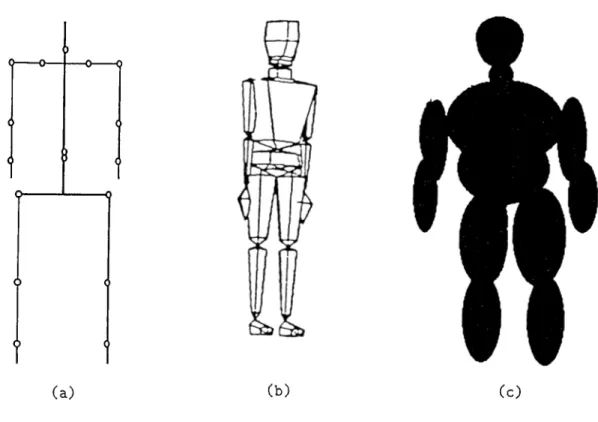
There are three general methods for modeling the human J^ody in 3-D [38] :

Stick Figures: These are like a skeleton and consist of a collection of line

segments attached by joints representing human body joints. Stick figures are unrealistic (figure 2.1(a)).

Surface Figures: These are basically stick figures surrounded by surfaces

that consist of planar or curved patches (figure 2.1(b)).

Volume Figures : Volume figures are the body models in which the body is

decomposed into several primitive volumes. Usually cylinders, ellipsoids, and spheres are used as primitive volumes (figure 2.1(c)).

(J--- 0---0--- 0

(a) (b) Cc)

Figure 2.1: (a) Stick model (b) Surface model (c) Volume model

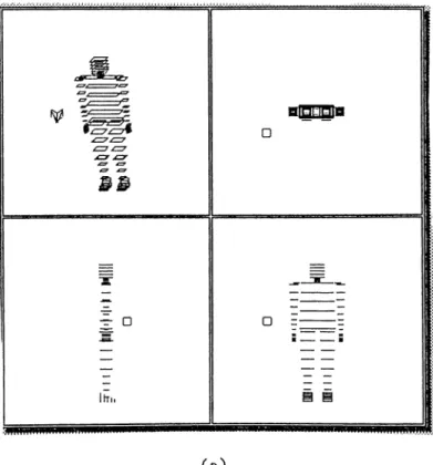
Practically, the level of detail included in a human body model is dictated by its purpose. The model that we are using is a kind of wire framed surface model, but without any planar or curved patch (figure 2.2). Actually each body segment is represented by a set of equidistant rectangles, one on top of the other, thus giving a surface feature. The choice for such a model is made because it requires less displaying time compared to most other surface models.

Figure 2.2; Human body model in AOHM

displaying. Stick model consumes the minimum displaying time but realism is almost totally absent because depths are difficult to evaluate and several movements like twists are impossible to represent. Thus our choice is almost a minimally acceptable one in terms of realism and almost optimal in terms of displaying time.

2.2

SEGM ENT MODEL

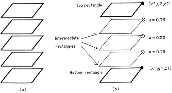
We have assumed the body segments to be rigid. Our body segment model is in fact like a rectangular box, consisting of five equidistant rectangles one on the top of the other. For each modification of the body segment one has to transform 20 (i.e. 5 x 4) vertices (figure 2.3(a)). Each transformation requires six multiplications and six additions (three for each x and y). What we are doing is that we transform 8 (i.e. 2 x 4 ) vertices (figure 2.3(b)), the vertices of the top and the bottom rectangles, and while displaying we compute the vertices of the intermediate rectangles by:

X = x l + u{x2 — a;l)

I

y = y l + u{y2 - y l)

where ‘u ’ is a parameter taking values 0.25, 0.50, and 0.75, and (x l.y l) and

(x2,y2) are the corresponding vertices of the bottom and the top rectangles.

(x2,y2,z2)

U = 0 . 7 5

U = 0 . 5 0

U = 0 . 2 5

(x1 ,y1 ,z1)

Figure 2.3: (a) Model of the body using five rectangles, i.e. 20 vertices are transformed, (b) A body segment model in which only 8 vertices are trans­ formed. # : Actual vertices that are transformed and 0 : Interpolated.

This parametric computation requires only two floating point additions and one floating point multiplication. Thus we save more than 500 floating point multiplications and more than 250 floating point additions in each modification of the orientation of the body.

In fact the choice of a model is application or purpose dependent. Our choice is reasonable for the purpose of interactive simulation tool. The body model typically consists of a tree structure, either body joints as nodes con­ nected by body segments or body segments as nodes connected by body joints. Both schemes have been tried, examples of the first scheme are CAR model and the original bubbleman model [23]. The second scheme is used by Boe- man (Boeing Corporation) [23], Bubbleman (University of Pennsylvania) [23], CAPE (Pacific Missile Test Center) [23], and others.

In the tree structure there is always a joint (or segment) taken as the root. In our model WAIST (upper torso) is selected as root joint (segment). This choice is natural as most of the limbs meet here. '

2.3

JO IN T MODEL

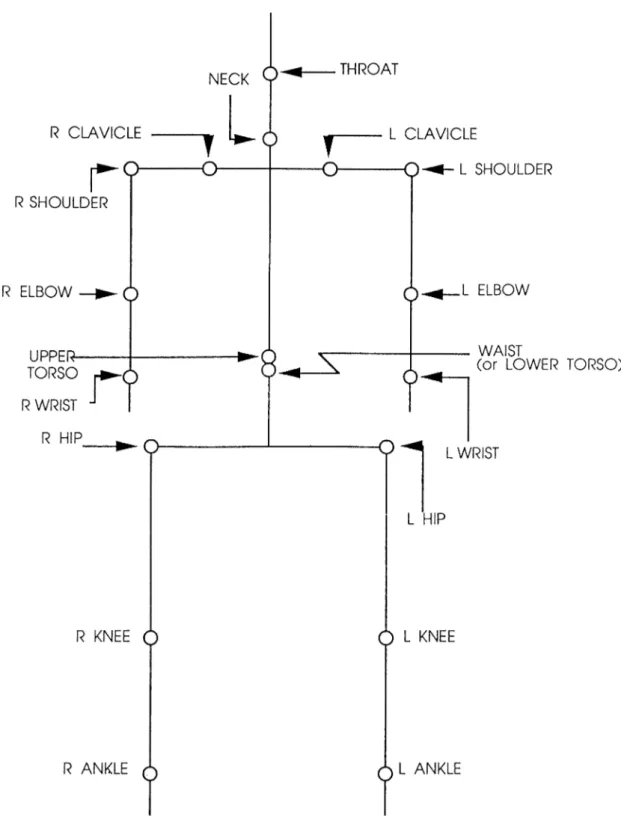
Modeling a joint means finding a computational model for representing the different types of motions depicted by them. The first step in modeling a joint is to decide on the depth of details to be included in the model, i.e., the number of joints the model will have. The more the number of joints the better the model is approximated. For all practical purposes, one cannot model to the depth of all the joints in the human body. In our model we have approximated with 18 joints (figure 2.4).

Human joints in general are basically comjrlex and idiosyncratic, as the limits of the degrees of freedom of their depicted motions are not constant. The limit of a joint parameter representing one degree of freedom may be a non­ linear function of the instantaneous values of the joint parameters I'epresenting other degrees of freedom of the motions of that joint. This interrelated nature of joint limits causes a real challenge while thej^ are modeled and leads to a trade-off between accuracy and uniformity [23].

The basic function of a joint is to connect two body segments (or links). Joints act as a pivot for segments to achieve different orientations while mov­ ing. The segment movement is restricted about a joint. During a single joint movement, one (proximal) segment is stationary and the other (distal) segment moves with respect to the proximal segment. Proximal means closer to the root (which only acts as stationary for all joints belonging to human body) in the hierarchy. In fact a segment can function as both ¡Droximal and distal if it belongs to two or more joints.

Every joint is assigned a unique identifier for referring them during speci­ fication of motions or body orientations. The joint identifiers used in AOHIM are ordinary names and not anatomical ones.

2.3.1

Joint M otions

In modeling joint motions it is better to reduce the freedom of motions embed­ ded in each joint to one or more independent parameters [23]. This eliminates

inconsistencies, especially while interpolating or generating inbetweens from the key-frames. To achieve this, a small number of motion types can be de­ fined and we can let the joints have one or more of these motions.

There are different types of joint motions with variable degrees of freedom [19]. A joint has up to three degrees of freedom [9]. Three degrees of freedom can be constructed and motions of lesser degrees of freedom can be achieved by restricting this model to a subset of degrees of freedom allowed. Thus, simple joints such as fingers (hinge joints), and complex joints, such as shoulders (ball- and-socket joints) can be simulated. A joint can move independently of all other joints except its parent and grandparents in the tree structure; this independent movement of the joints actually defines the joint’s actual trajectory.

Usual anatomical concepts about joint motions cause ambiguity in model­ ing. Thus the mechanical approach of revolute and spherical joints plays an significant role in describing joint motions of the human body.

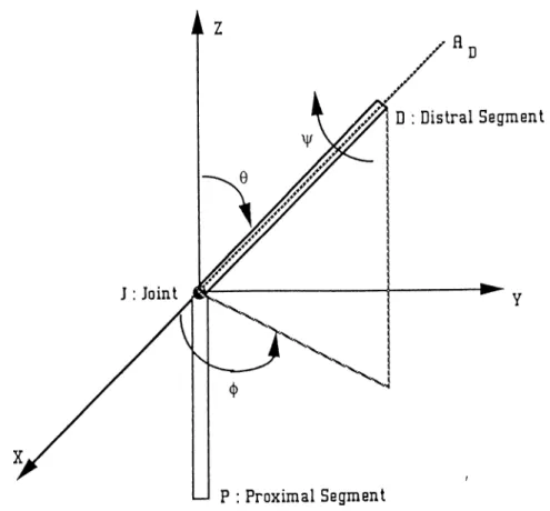
Figure 2.5: Computational model of a joint

10-A spherical joint has three degrees of freedom, and the three parameters (or variables) used can be defined by numerous means and using a different coordinate system (figure 2.5).

The proximal segment P is fixed in the coordinate system (spherical in AOHM) originating at the joint J , and axis Ad of distal segment D is a line through the origin. The position (or orientation) of the distal segment is given by (j), 9, and 'll), (j) and 9 give the description of the direction of the axis Ad·,

and Ip describes the amount of rotation of distal segment D about Ad- The

type of motion achieved by the variation of first two parameters (^, 9) is called

spherical motion, as it specifies the position of the sibling joint Js of the joint J

at the other end of distal segment D in spherical coordinate system with a fixed radius or r of spherical coordinates (r, 9, <f>), and the motion by (t/>) is called

twist [23]. The motion depicted by shoulder having three degrees of freedom,

needs to be assigned both of these motion models. For instance, positioning the elbow (Js) by modifying the state of shoulder J joint is an example of spherical motion, ip corresponds to the twisting of the upper arm about its axis, twist motion.

Besides spherical and twist motions, there is another important and com­ mon motion type known as flexion motion. Examples of flexion motions are seen in the knee and elbow flexion. The distinction between flexion and twist is useful for clarity of visualization [23]. Flexion motions can be modeled via the spherical motion model by restricting it to only one degree of freedom (9) as flexion motion has only one degree of freedom. Thus we have the following three joint motion models:

• Spherical

• Twist

• Flexion

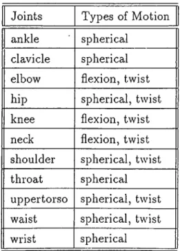
To understand the nature of motions depicted by the joints given in figure 2.4 or about the joints included in the human body model AOHM implemen­ tation, table in figure 2.6 is provided:

Joints Types of Motion ankle spherical

clavicle spherical elbow flexion, twist hip spherical, twist knee flexion, twist neck flexion, twist shoulder sj^herical, twist throat spherical uppertorso spherical, twist waist spherical, twist wrist spherical

Figure 2.6: Table of human body joint motions

In AOHM only spherical and flexion are included; we shall incorporate twist in the near future.

2.3.2

Joint Limits

We need to consider joint limits in order to make the motion of the human bod}' more realistic. If it had not been there, the animator would have oriented the human body in any way he would have preferred, treating the human body like any linked body without any restrictions on joint, and many orientations would have appeared that are not possible.

Joint limits to be discussed in this section is based on the joint motion models mentioned in the previous section, namely, flexion, twist, and spherical.

Flexion and twist motions have a single degree of freedom, so joint limits are just constants (a minimum value and a maximum value). These constant limit values are based on the assumption that the extreme values (limits) do not depend on the current value of any other joint variable; this is not true

in general. But for many practical purposes, this assumption does not cause much trouble.

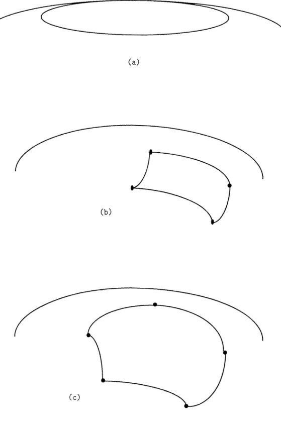
Joint limits for spherical motion is not a trivial one. Actually the distal end of the distal segment is forced to lie on a sphere about a joint. On imposing joint limits the distal end is restricted to lie within some patch on the sphere. The boundary of this patch is called the joint limit curve. When the two variables are treated independently, curves of figures 2.7(a) and (b) are observed. In figure 2.7(a) the first parameter [6) is restricted to certain values (maximum and minimum) and the second parameter {(j)) is allowed to span through the whole of its domain. In figure 2.7(b) both of the parameters have certain extreme values (maximum and minimum). These types of limit approaches are not close approximations to the actual limit boundaries of human joint limit curves but they, being very cheap to implement, are widely used and we have also implemented this scheme in AOHM. Figure 2.6(c) shows another approach which is a closer approximation to the actual case. In this scheme the joint limit boundary is approximated by a spherical polygon, consisting of points on the sphere connected by arcs.

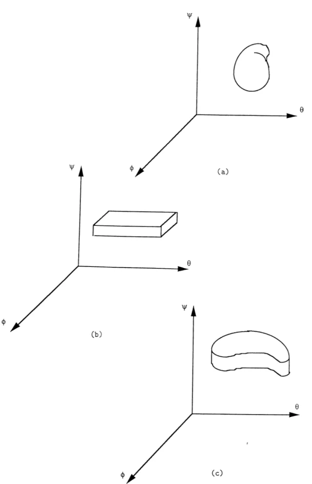
For a joint depicting both spherical motion and twist motion (a shoulder is an example of such a joint), different joint limit boundary approximation approaches can best be understood by describing the set of allowable values for the joint variables in the 3-D configuration space defined by the variables (^, i?, and Ip. In most general case where all the joint limits are dependent on the current values of other variables (parameter), the configuration is an arbitrary blob in space (figure 2.8(a)). In figure 2.8(b), the most simple case is shown when all the three joint limits are constant values, a maximum and a minimum. In figure 2.8(c) third parameter (ip), i.e., twist motion has constant value limits, but the limits of spherical motion are not constant but interrelated.

Figure 2.7: (a) Independent joint limits, (b) Another independent joint limits, (c) Joint limit curve approximated by a polygon on the surface of the sphere.

Figure 2.8: (a) All joint limits are coupled, (b) All joint limits are independent, (c) (f) and ^ limits are coupled but limit is independent.

3. H U M A N BO DY A N IM A T IO N

“Above all, animation is the art of movement. The accomplished animator can bring life to just about anything - a series of drawings or a tin can” [24].

The etymological definition of ‘Animation’ can be stated as ‘giving life to something’; that something can be a still picture drawn manually on a piece of paper or by computer on a display device. So for our purpose ‘Animation’ is making the pictures of human body drawn on a still frame appear to move, making use of the persistence of vision phenomenon of the human eye.

When computer animation is discussed a few questions come to mind: What will be the animation technique at display level? How one is going to show the still pictures? W hat will be the animation technique at the level of creation of

sequence frame (sequence frame is the set of still pictures to be displayed while

animation)? How each of the frame of the sequence is going to be generated or to put in practical terms? How the motion is going to be specified, so that the burden could be brought to an acceptable ratio?

3.1

A N IM A TIO N TECH NIQ UES

There is a variety of techniques for animation, among these we shall be dis­ cussing those which can be considered for the animation of articulated bodies like human body. As mentioned above, animation techniques can be and should be explored both at the display level and at the level of frame sequence creation.

There are basically two animation techniques as far as the display of a 3-D picture is concerned:

• Frame by frame

• Draw and display

In the first technique the whole frame sequence is prepared and put into the memory and then each frame is displayed one by one. This technique requires large memory for even short animations. A partial solution is to not save every frame, but rather save the differences between the consecutive frames. This slows down the rate of display.

In the second technique, each frame of the sequence is prepared when it is to be displayed. Hardware plays an important role because the drawing mechanism needs to be really fast, to achieve smooth and realistic motion. An important issue to be noted here is that when the frames are to be drawn, and how much information is ready in the created frame. This preprocessing can be anything like calculating the color values, or transforming some data points, or even finding a suitable transformation for the frame. The more manipulation a frame requires before it is ready to be drawn, the slower the display speed will be. Fast animations can be achieved by completely preprocessing the frame information beforehand. For complex figures like human body, to do all the manipulation beforehand is not quite feasible from the memory point of view, especially if the sequence is permitted to be modifiable.

As far as the generation of frame sequence is concerned, we propose the following classification of animation techniques, especially for human figure or any articulated body in general: •

• Goal-directed animation

• .A.lgorithmic animation

• Procedural animation

3.1.1

Goal-Directed Anim ation

All frames of the motion sequence for a particular motion is generated by the machine in response to user’s simple English-like commands, such as ‘walk', ‘ru n ’, ‘jum p’, etc. [11]. The motion planning and control is done by the machine and the animator does nothing except specifying a command. We know that sa.}»^, human walk, is not a unique motion; rather there are hundreds of different kinds of walks depending on the step size, speed, personal dimensions, etc., so just giving a command like ‘walk’ we cannot achieve different types of walks. As a solution the concept of parametric goal-directed animation is used. Here, together with the command ‘walk’ some parameters like step-size, speed etc. [7] are allowed.

In goal-directed animation, be it parametric or nonparametric, the animator gets rid of the planning and control of human motion and motion in general. In this technique the main problem is how the machine is going to plan and control the motion.

Procedural methods can be used which has a knowledge base for motion [34], but this is not very realistic for most cases. This is because the quality of motion depends on the amount of information embedded in the knowledge base. This issue becomes more critical when one is trying to develop a general- purpose tool for human motions, as a huge amount of information is needed. This technique can be implemented as a language base [11], or with parametric functions.

Kinematic control is another method and is the one mostly used in designing control mechanisms for human motion planning. Although this also is not realistic, it still gives acceptable performance. The basic tools of a kinematic approach is position, displacement, and velocity of the object. Sometimes acceleration is also used. In kinematic approach forces and torques are not considered.

Dynamic control is the one that gives the most realistic results but compu­ tationally it is expensive. In dynamic control, besides position, displacement, and velocity, energy, force, and torque which tend to cause the motions are also

considered and the center of mass plays an important role in motion planning. But calculating the center of mass of human figures is not trivial The main reason for dynamic approach being computationally so expensive is the typical structure of human body, the articulated nature of body segments. So mass analysis is needed to be done for each body segment individually; same is true for force and torque calculations. Apart from being expensive, there is another problem with this technique: the animator has to supply the information about the forces and torques.

To get a flavour of the dynamic approach let us consider the following:

An angle x of a joint is to be modified to y. One can calculate that torque T applied to a joint by [1]:

T(x) =

The parameters a and ¡5 determine the strength of the torque applied at the joint and they can be controlled by the animator in parametric goal-directed animation. In general, one can divide a motion sequence in phases either for the whole body or for groups of body segments and for each phase one can derive a system of non-linear equations by using the Lagrange method. The Lagrange equations for a system with n degrees of freedom can be written as:

_d m \ _ ^

^

K

This is used in [7]; what is done is that the walk motion of the legs are divided into two phases, viz. stance and swing. Stance means that the leg is touching the ground and swing means that the leg is in motion, that is, off the ground. The Lagrangian method is applied to the individual phases of the walk motion, namely stance and swing. The phase analysis is first done independently at the

level of body parts. At the end of this analysis the dependencies are propagated to other related body parts in terms of forces and torques.

Practically the dynamical control is never used as the sole control mecha­ nism, rather kinematic control is used and decorated with dynamics whenever needed [7, 8, 15, 16, 33, 43, 44].

3.1.2

Algorithm ic Anim ation

Motion is described algorithmically. Actually physical laws are applied to pa­ rameters of the human body, e.g., joint angles. Control of these laws may be provided to the system by procedural methods as in MIRA [14] or by inter­ actively as in MIRANIM [14]. In fact one can specify almost any law for the parameters after building a reasonable input mechanism.

These laws may be based on kinematic approach, i.e., positions, displace­ ment, and velocity, or dynamic approach, incorporating force and torque in addition to the kinematic criteria. As discussed before, dynamic approach is expensive so here also mostly the laws based on kinematics are applied and dynamics is incorporated whenever needed. These laws can also be specified as functions defining the trajectories of a joint in a motion sequence. But for these a sound understanding of the trajectories of the human body joints during a particular motion is necessary [3, 27, 28, 29].

Whatever law is used, algorithmic animation is expensive in general because a computation of the algorithmic function is done for each parameter of every joint while generating a single frame and same is true for ea.ch frame of a whole motion sequence.

Algorithmic animation, being computationally expensive, is hardl}^ ever- used. Instead, in most applications it is integrated with other techniques which are comparatively cheaper. This is discussed in section 3.2.3.

3.1.3

Procedural A nim ation

This technique includes describing animation by an animation language ( e.g., CINEMIRA-2 [13]) or by scripts (in script systems). Procedural animation’s main basis is the knowledge base of motions, and the language, functions, and scripts all consult and depend on it. There can be different abstractions for the level of description of motion in procedural animation; the highest level is the same as goal directed animation.

Procedural animation, being heavily dependent on the knowledge base, can­ not be used in tools designed for the wide range of human motions, as it is difficult to include all the details of the whole span of human motion.

3.1.4

Key-Frame A nim ation

Key-frame animation is one of the oldest animation techniques still in use because of its inherent nature th at suits interactive environment. In this tech­ nique the animator typically orients and positions the human body interac­ tively, designating a sequence of configurations, called the key-frame and in most of the cases also describing the time instances of their occurances. Then the system automatically generates the intermediate frames, known as inbe-

tweens, based on the sequence of key-frames supplied by the animator.

Interpolating between related key images allows the animation of change of shape and distortion in general, and change of orientation and position in the case of human motions. Actually.it permits a direct method for specifying the motion or action, in contrast to the mathematically defined distortion that requires trial and error. A desired result is achieved by iterated experiments. One quality observed in key-frame animation is that it is in a way analogous to conventional animation, making it easier for a classically trained animator.

Image-Based Inbetweening

The inbetweens are obtained by interpolating the key-frame images. This tech­ nique is called image based key-frame animation by Steketee and Badler [35] or shape interpolation by Zeltzer [13]. This is an old technique introduced by Burtnyk and Wein [13].

Parametric Inbetweening

This is a better way to compute the inbetweens. Instead of the images, the joint parameters of the human body are interpolated. This is called paramet­

ric key-frame animation. It is also known as key-transformation animation.

In a parameter model, the animator creates key-frames by specifying the ap­ propriate set of parameter values, and then the parameters are interpolated and images for the inbetweens are obtained from the interpolated parameters. Parametric key-frame animation is actually the technique used in AOHM.

There are a few issues needed to be resolved while implementing this tech­ nique. First, how will the animator specify the motions? How will the animator produce key-frames? Will he (and not the machine) modify the joint param­ eters to yield an orientation of human body in a key-frame? .Another way can be that the animator will just give a command and the s3'^stem will do all the job and prepare all the key-frames for the animation, as in goal-directed animation.

Second, we have the problem of interpolating the parameters of the body specified in the key-frame for yielding inbetweens. So one needs to e.xplore some methods while designing a tool based on key-frame animation.

Third, the animator has almost no control over the inbetweens, the

in-I

terpolation of the key-frames. Quite often unrealistic motion results in the inbetweens if special care is not taken. Thus this issue cannot be neglected if one is aiming at designing a tool which should not produce very unrealistic motions.

3.2

PA R A M E T R IC K EY-FRAM E A N IM A TIO N

This is the technique used in the implementation of our AOHM. In param et­ ric key-frame animation, the animator interactively orients and positions the human body for the generation of each frame, called key-frames, i.e., some important orientations and positions of the human body at selected intervals during the time span of a desired motion. Orienting and positioning the human body means specifying the value for body parameters like a particular degree of freedom variable of some joint, directly or indirectly. Directly means mod­ ifying each joint parameter explicitly for generating a key-frame of a motion sequence. This is a laborious task for the animator and the machine almost has nothing to do, this is the lowest level of motion specification. Indirectly means some higher level of motion specification that is finally translated into the lowest level by the machine, thus parameters are modified implicitly.

Once the animator completes the creation of key-frames for the motion sequence, the system automatically, based on some interpolating method gen­ erates the rest of the frames, called inbetweens, i.e., the frames lying between the consecutive key-frames.

There is a problem with this technique: The animator does not have total control over the inbetweens generated by the system. It is almost impossible for an interpolating method to be intelligent enough to produce the inbetweens realistically for a wide range of motions such as the span of human motions. Thus there is a need of some mechanism to upgrade the quality of the inbe­ tweens.

Parametric key-frame is chosen for AOIIM because it is inherently very suitable for interactive motion specification which is one of the main themes of AOHM. Intelligent motion controlling and planning algorithm is also not really needed in this technique.

3.2.1

M otion Specifications

Motion control is a central problem in computer animation [43]. The spec­ ification and control of motion in human figure animation has always been a challenge [7], and many different approaches are being made to resolve it. Badler [3] approaches the issue by exploring the criteria to a good or accept­ able movement representation. Badler [5] also suggests natural language as an artificial intelligence application to motion specification. English-commands [11] and parameterized goals [7] suggest the motion specification in the highest level. There are other approaches like using functions [43] and body orienta­ tions and positioning [9] as lower level specifications.

After analyzing all the above researches and suggestions for motion speci­ fication levels one thing is worth noting; as the motion specification level gets higher, that is to say as the animator’s job is simplified, the computer does more work and the motion control and planning algorithm gets more intelli­ gent and complex. Moreover, the animator’s control over motion generation becomes less. Thus if in a particular motion that is supported by the sys­ tem in a high level of motion specification the animator desires to have some minor adjustments, then it is almost impossible, especially if in the parameter­ ized goal approach the available parameters cannot support that modificcition. Moreover in high level of motion specifications wide range of motions cannot be supported. It is also worth noting that if the animator is given all the control i.e. while generating a key-frame play with any parameter (degree of freedom variable of joint motion) of the human body and no higher level mo­ tion specification is supported, then even for the generation of a single motion frame the animator would have to do very laborious work and the machine would almost be idle, but here almost any motion is possible. Thus there is a trade-off between the level of control and the level of ease the animator should have in motion specification.

Considering the above trade-off a need for a tool that supports different abstractions of motion specification is felt and for the implementation of such a tool there is a need for a taxonomy of motion specification levels. We propose the following taxonomy:

• Joint parameter modification

• Joint positioning

• Semi goal directed approach

• Goal directed approach

As we go down the classification the level increases, the animator’s job gets simpler, and the computer’s work gets more complicated.

J o in t P a r a m e te r M o d ificatio n

This is the lowest level of motion specification. Here the computer does not have to do any translation of the animator’s command, it is in the most prim­ itive form. But for specifying motion, rather orientation and position the animator’s job is burdensome.

T ran sla tio n : This primitive specification is stated as a triplet:

T = (G, ty, G)

where and G displacements. Ax, Ay, and Az in coordinates x, y, and z of the human body (as a whole articulated object) defined in Cartesian coordinate system, respectively. It should be noted here that translation cannot be specified for a joint or segment as they make up the articulated figure.

R o ta tio n : This is the second type of primitive specification of motion and is the most used one. It can be specified as

R = (joint-name, angle, axis)

where ‘joint-name’ is the joint identifier whose state is desired to be modified, ‘angle’ gives the amount of change in the value of a joint' parameter desired, and ‘axis’ actually determines which degree of freedom should be modified. In AOHM axis takes only two values; 1 to specify 9 and 2 to specify <j). A state is

a set of values of the parameters (0, (f>) of joint motion. Now to understand the state and how the state is modified or in other words how primitive specification ‘rotation’ is made, consider figure 3.1((a) and (b)). The joint parameters are actually spherical coordinate ordinates.

In figure 3.1(a) the joint ‘RSHOULDER’ (right shoulder) has a state S\{0 = 40°, (j) = 65°) and rotation

R = {RSHOULDER, -20°, 1)

changes the state from Si to S^ {0 = 20°, (j) = 65°). Actually the primitive specification says that change the state of joint ‘RSHOULDER’, decrementing the value of its first degree of freedom by 20°.

The coordinates of joint or location o-f joint in space given by triplet (x, y, z) is not included in the state definition. This can be better understood if figure 3.2((a) and (b)) is studied.

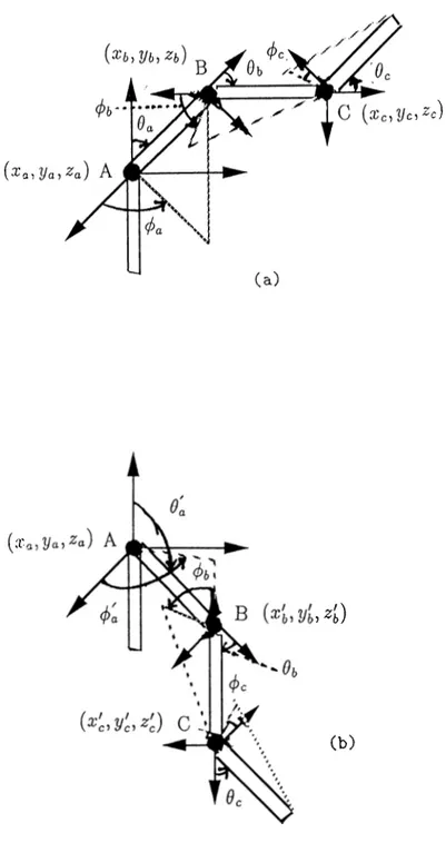
In figure 3.2(a) there are three joints A, B and C with states {Oa, 4>a)·,

{0b, (j>b), and {0c, (f>c), and joint positions { X a , J/a, Z a ) , {xb, Vb, Zb), and { X c , IJc·, Zc)

respectively. The joints A, B, and C constitute a linked configuration, being a part of linked figure like human body. The joint B is connected to the joint A through the body segment AB. A similiar relation exists between the joints B and C. Now modifying the state of the joint A to {0'^, the coordinates of the joint B will get modified to {x'b, y[, z^) and that of C to (a;(,, y', z{.). Here it is worth noting that the relative orientation of the body segment BC with respect to the body segment AB is unchanged, thus the state of the joint B is unchanged. Similarly the state of the joint C is unchanged. This isolation of position (a;, y, z) from the state {0, (j)) is made because when the position changes with respect to its siblings, it only means that one of its parent or grand parent joint has changed its state or in other words some comparatively proximal joint has modified its orientation. Thus any change in the state of a joint is propagated through its siblings to the end-effectors by position change.

In AOHM joint limits are also implemented but in their simplest form and we hope to make it closer to realistic joint limit curves in the future. Joint limits for each of the joint parameters (degree of freedom) is a pair of maximum

Figure 3.1: (a) Initial state of the joint with 9 — 40° aqd <f) = 65° (b) Final state of the joint after the rotation R = (RSHOULDER, —20°, 1) i.e. 0 = 20° and ^ - 65°.

(b)

Figure 3.2: (a) Initial states and coordinates of the joints A, B, and C (b) Final state of the joint A and different coordinate values of the joints B and C.

and minimum. Whenever a primitive motion specification is made the system checks whether the new value is within the limits. If it is, then the value of the joint parameter is modified. Otherwise, a message is given to the animator that the limit is violated and the modification is not allowed.

There is a problem of induced twist in the body segments or joints; when for a joint having some value its ‘çi»’ value is modified by a reasonably large value, some amount of unwanted twist is introduced because of the transforma­ tion. This should be removed by some corresponding inverse transformation. Finding this inverse transformation for neutralizing the unwanted twist is easier if the joint model contains twist motion as one of the degrees of freedom.

It is clear from the above discussion of primitive specification of motion that even for bringing the human body to a desired simple orientation the animator has to perform a laborious task. So there is a need for a higher abstraction of motion specification that would help the animator orient the human body with less work.

J o in t P o sitio n in g

As a solution to doing less work while orientation and positioning the body for a key-frame, the system may have the provision for positioning a joint to a desired or goal position in the world coordinate system.

The goal ‘g ’ is defined as a triplet {xg,yg,Zg) and the ‘jo in t id e n tifie r’.

{xg,yg,Zg) is specified interactively by the mouse. In AOHM the animator can

see the goal position in all the three planes x-y, y-z, and z-x while specifying it (figure 3.3(a)).

After the goal position is specified and the joint is identified (figure 3.3 (a)), the system solves for the related joint parameters and if a solution exists it positions the identified joint to the desired goal position (figure 3.3(b)).

Positioning a joint which is attached to torso or the main body means a

II

translation. Positioning a joint whose parent is attached to torso means that the goal position should lie on the spherical surface spanned by the identified

/=17^=3^

ItTit

(a)

s m

(b)

Figure 3.3: Isometric, top, front, and side views, (a) Gbal position and the body with unpositioned joint (b) Body with joint positioned.

joint when its parent joint is treated as the center of the sphere. Moreover, the goal position should lie within the joint limits. There is yet another positioning in which the identified joint’s grand parent is attached to torso or it is fixed. This means that we have more degrees of freedom in positioning the joint. Examples of such joints are wrists and ankles for our model. This type of joint positioning is more challenging and requires some dedicated methods, especially if joint limits are to be considered.

There are many algorithms for positioning a joint or finding the joint pa­ rameters of other related joints for positioning an identified joint. Most algo­ rithms are explored in industrial robotics and thus do not take into account the constraints of joint limits which is a important issue in our case.

When joint limits are ignored and a joint is identified to be placed at a goal

(xg, i/g, Zg), tfic valuos of the joint parameters of other concerned joints (joints

whose states need to be modified in order to place the identified joint at the desired goal position) can be calculated by open chain inverse kinematics. In open chain inverse kinematics a linked body is presented with one end fixed and the angle values for all the joints in the linked body is calculated in order to position the other end to a desired position.

Another step towards simplifying the anim ator’s job would be providing a facility of positioning multiple joints to respective multiple goal positions. Usually not all the identified joints can be put precisely to their respective goals, because it is difficult for the animator to visualize the modified states of the joints when one identified joint is positioned to its goal. Thus for multiple joint positioning a mechanism for approximating the positioning of the joints should be designed and supported. An approach of weighted goal [2] has been proposed for this case. The concept of weighted goal says that whatever be the mechanism of positioning the joints, care should be taken that the joints having higher goal weights should be approximated with lesser error, i.e. closer to their respective goal. For a detailed discussion the reader can refer to [2] where joint limits are not considered.

A method for positioning a single joint with the constraints of joint limits is implemented in AOHM. We developed this method based on the one discussed

in [23].

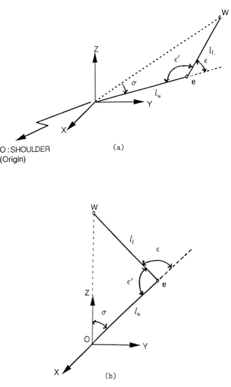
To understand the algorithm for positioning the joint (end-effector) let us take the case of positioning the wrist of a 3-D arm (body segment consisting of wrist, elbow, and shoulder joints) (figure 3.4).

The shoulder is taken as the origin of the coordinate system, and let the positions of the elbow and wrist be ‘e’ and ‘W ’, respectively (figure 3.4).

The arm has four degrees of freedom, two each for the shoulder and elbow joint, and the goal has three parameters. There is one degree of redundancy. Thus there is no unique solution rather a set of solutions if there exists any at all.

In figure 3.5 it can be seen that the problem is actually to find a value for the elbow angle e and a value for the angle (p, such th at the states of shoulder and elbow joints are within their joint limits. The angle (j) can be defined as the orientation of the plane formed by 0,e, and W w.r.t. the x -ax is when the z-axis is taken as coincident to the imaginary line joining 0 and W. It is further assumed that the axes of the coordinate system origined at shoulder joint have such orientations that when the imaginary line joining 0 and W i.e. OW is transformed with T~^ to coincide with the z-axis of the coordinate system of the shoulder joint, the two systems should coincide. Finding the e and (p angles suffices because shoulder joint 0 is inherently fixed and the wrist joint is fixed because of the goal constraint.

Basic Algorithm :

• 1. First check if ||OT'F|| < (sum of the upper and lower arm lengths).

• 2. Find elbow E angle e (elbow’s 6 angle) and check it against the joint limits of the joint elbow.

• 3. Find an expression for CIR(<^), a vector function that gives a circle on which the elbow is constrained to lie by the shouldqr position 0 and the goal position W of the wrist.

• 4. Determine the arc ARC1((^) on CIR(^) to which the elbow is restricted

w

w

Figuie 3.4. (a) Aim model and the plane of the arm (b) Goal line segment

by the (j> limits of elbow joint. Arc A RCl(^) means a subset of the domain of (j) which is permissible by cf) joint limits of elbow.

• 5. Determine the arc or set of arcs ARC2(<^) on CIR((?i') to which the elbow joint E is restricted by the shoulder joint limits.

• 6. Take the intersection of arcs A RCl(^) and ARC2((^). choose some value of <j> and calculate the state of shoulder and elbow joints.

Now let us discuss each of these steps in detail:

1. G oal d istan ce : Checking whether the goal position Zg) is

very far or within reach, is very simple. From figure 3.5 one can say that,

\\W\\<lu + h

means within reach, otherwise too far, i.e. no solution possible. VE|| denotes the magnitude of the vector W from shoulder to the goal as wris: position, and // are the lengths of the upper and lower arms respective!}'.

2. Elbow 6 angle : Consider figure 3.5, interior elbow angle t, can be obtained from the law of cosines as

cose' = (/2 + i f - | | W f ) / ( 2 U , )

Here t denotes the 0 angle of the elbow and can be obtained as

t ■= — (!

The value of e should be checked against the limits of the elbow's 0 angle.

3. E lbow circle: Here an expression for the parametric description CIR((?i') of the elbow circle (figure 3.6) is required. It is easy to find eri expression for CIR°{(I>) shown in figure 3.6(a), and then apply a transformation T·^ to

CIR°{4>) to yield

CIR{<I>) = T ^ * CIR°{<t>) (₁)

where represents a transformation m atrix that maps z-axis in figure 3.6(a) to the vector W in figure 3.6(b). Thus if we apply this transformation to each point on the CIR°{(f>) we can obtain the corresponding points P„·· on CIR(<;i').

w

(Origin)

W

Figure 3.6; Elbow circle with wrist vector W on (a) Z-axis (b) Arbitrary orig­ inal position

To find an expression for CIR°{<f>), a should be determined, a can be calculated (figure 3.5):

cos<. = (||W'|p + /2 - ;? ) /( 2 ||iv ||y

A sphere of radius around an origin can be represented as: / sin 9 cos 6 \

(2)

S {0 A ) = L sin sin 4> cos 6

(3)

Putting 9 = a \TL equation 3, we get CIR°{<I)) as: /

sin cr sin <f) cos a sin a cos (f> ''

CIR°{<f>) = lu

Final expression for CIR{<f) can be obtained with equation 1.

(4)

/

4. E lbow jo in t (f) lim its: In this step an arc ARC1{4>) is determined by restricting the (j) domain of CIR{<f>) with the (j) limits of the elbow joint. The arc can be obtained simply by considering the upper and lower limit values of the (j) degree of freedom of the elbow joint, the corresponding '(/>’ values in the

(f) domain of CIR(<f)) is noted and ARCl{(f>) is obtained.

5. S h o u ld e r jo in t lim its: Here a subset of the domain of parameter of the parametric description of the elbow circle, in terms of a set of arcs,

ARC2{(f>) is to be determined such that each of the 4> belonging to this subrange

satisfy the joint limit constraints for each of the two degrees of freedom 9 and

(f) of the shoulder joint. To understand the issue let us consider the problem

geometrically.

In figure 3.7 CIR{4>) is a circle in 3-D lying on a sphere of radius and center 0 , the shoulder joint (origin). The joint limits can be represented in spherical coordinates as

f[ = _{^lowlimt ^lowlim)}

T2 =

rz = (/u) ^uplim·) ^uplifTi)

It can be seen (figure 3.7) that the four joint limit vectors of shoulder joint

Figure 3.7: Elbow circle and the joint limit boundary.

constitute a spherical polygon Pol-lim (ri,T 2,ra,T4, n ) on the surface of the sphere of radius and center 0 . Thus there may exist intersections r,i and ?’,-2 between the circle CIR{(j>) and the spherical polygon Pol-lim, i.e. the existence of the arc ARC2{(j)). The problem of finding the intersections can be better understood by considering figure 3.8(a).

W hat we mean by finding ARC2((f>), is that, determine the subset of the loci of elbow circle, CIR{(f) which lies inside the shoulder joint limit, spherical polygon Pol-lim, figure 3.8((a) and (b)). In figure 3.8(b) we see that ARC2{(f)) can be a set of arcs instead of being just a single arc. Figures 3.8 (c) and (cl) suggest that in case of no intersection found, a test should be made to find if the whole of the circle is inside the spherical polygon Pol-lim, figure 3.8(d), or totally outside, figure 3.8(c). This test is a very simple one, all one has to do is take any point on CIR{(j>) and test it against each of the extreme values (limits) of each of the shoulder joint’s degrees of freedom.

For each of the intersections, r ,’s we know their magnitudes are and the

$ value is V ’. Thus, the problem reduces to finding a set of <j) pairs <f>max)

Figure 3.8: Elbow circle and joint limit boundary (a) Two intersections (b) Four intersections (c) No intersection (joint limit boundary inside) (d) No in­ tersection (joint limit boundary outside)

which correspond to the arcs in the set of arcs in ARC2{(f>)^ i.e.:

(j) domain of ARC2{<f>) is _{m a x ) ? ’ ’ *} 5 4^ km ax)'\

The solution of the problem will be simplified if the circle CIR{(f>) and the spherical polygon Pol-lim are transformed by where T~^ is the

transfor-—f

mation th at maps the vector W to z-axis of the shoulder coordinate system. Thus we have the situation of figure 3.9. For simplicity of notation we shall still refer to these transformed loci cis CIR{<f>), ARC2'{(f>), and Pol — lirn' are the ARC2{(f>) and Pol-lim.

Figure 3.9: Elbow circle and the joint limit boundary, both transformed so that the circle’s axis of rotation coincides with the Z-axis of the shoulder.

The problem of finding the intersection between the circle CIR{(f>) and the spherical polygon Pol-lim can be thought of as finding the intersection of the circle CIR{(j>) with each of the arcs 7^2> respectively. Thus availability of a method to calculate the intersection of the circle on the sphere with an arc on the same sphere suffices our purpose, we, therefore, state our intersection method designed for this purpose.

Before discussing the method for finding the intersection between the circle

CIR{<I>) and the arc n r 2, let us see the different cases of how and when the

intersections exist. We have classified the situations as shown in figure 3.10. For analyzing the different situations in figure 3.10 we need to state a definition:

D efin itio n : A point r (vector r) on the arc fxf^ is inside circle CIR{(j)) if the

6 angle of r, is less than the constant 6 angle, cr^ the angle of each point on the loci of the circle CIR{(f)), otherwise we shall say r is outside the circle.

D ifferen t cases:

(i) One edge point, 7’i is inside and one edge point, T2 is outside circle

CIR{(f>) so there exists one intersection point, figure 3.10(a).

(ii) Both edges r-y and V2 of the arc 7^2 a.re either inside or outside

the circle CIR{(j>) so:

(a) 3 no intersection (figure 3.10(b)).

(b) 3 two intersection (figure 3.10 (c)).

(c) 3 two intersection but a tangent point (figure 3.10(d)).

When cases (ii)(a) or (ii)(c) occur we have to do nothing; we simply ignore that arc and skip to the next one in polygon Pol-lim.

In case (ii), we need a mechanism to differentiate between the respective situations (a), (b), and (c).

For cases (i) and (ii)(b) we need to solve for the intersections as follows:

M e th o d : in te rse c tio n s b etw een an arc a n d a circle

For cases (i) and (ii)(b) a general method can be found which actually always finds two intersection points (vectors) of the two circles CIR{(f)) and

ARCCIR{cc), where the circle A R C C I R { a ) is obtained by extending the arc

7^2 from both sides on the spherical surface. Then if case (i) exists simply ignore the unwanted solution (intersection point), otherwise take both the in­ tersections for case (ii)(b). Although this algorithm is general, we shall use the notations in compliance with our purpose.

(b)

Figure 3.10: Elbow circle and an arc as one of the sides of the joint limit spherical polygon (a) One edge of arc inside and one edge outside the circle and one intersection, (b) Both edges inside or outside and no intersection, (c) Both edges inside or outside and two intersections, (d) Arc tangent to the circle.