Government spending and fiscal rules in a simple endogenous growth model

Government Spending and Fiscal Rules in a Simple

Endogenous Growth Model

SAKIR DEVRIM YILMAZ

103622006

İSTANBUL BİLGİ ÜNİVERSİTESİ

SOSYAL BİLİMLER ENSTİTÜSÜ

IKTISAT YÜKSEK LİSANS PROGRAMI

Tez Danismani: Ege Yazgan

2007

Government Spending and Fiscal Rules in a Simple

Endogenous Growth Model

(Basit Bir Endojen Buyume Modelinde Devlet Harcamalari ve

Mali Kisitlamalar)

SAKIR DEVRIM YILMAZ

103622006

Tez Danışmanının Adı Soyadı(İMZASI) : EGE YAZGAN

Jüri Üyelerinin Adı Soyadı (İMZASI) : ...

Jüri Üyelerinin Adı Soyadı (İMZASI) : ...

Tezin Onaylandığı

Tarih

:

...

Toplam Sayfa Sayısı:40

Anahtar

Kelimeler

(Türkçe)

Anahtar

Kelimeler

(İngilizce)

1)Mali

Kisitlamalar

1)Fiscal

Rules

2)Endojen

Buyume

2)Endogenous

Growth

3)Altyapi

Yatirimi

3)Infrastructure

4)Simulasyon

4)Numerical

Analysis

ABSTRACT

This thesis attempts to analyze the implications of imposing a Golden Rule of public finance (where the government is allowed to borrow for infrastructure investment) and a standard Primary Surplus Rule on fiscal balances and growth in an endogenous growth model with productive public infrastructure and health spending. I assume a closed economy with no money creation so the government’s only source of revenue is taxes on output and interest income. Due to the high complexity and non-linearity of the model, numerical simulations are performed to analyze the transitional dynamics following various shocks. It is shown, under the calibrated parameter values that the Golden Rule performs better in terms of growth and speed of convergence than the primary surplus rule. Further, the numerical simulations also show that constraining the government to borrow for other forms of productive spending such as health through fiscal rules may entail significant growth and debt-reduction costs.

OZET

Bu tez Kamu finansmaninin altin kurali olarak da bilinen ve devletin yalnizca altyapi yatirimlari icin borclanmasina olanak saglayan “Altin Kural” ile standart faiz disi fazla hedefi mali kisitlamalarinin buyume ve kamu finansmani uzerindeki etkisini altyapi ve saglik harcamalarinin uretken oldugu endojen bir buyume modelinde incelemektedir. Modelde para olmamakla birlikte develetin tek gelir kaynagi uretim ve faiz geliri uzerinden aldigi vergi olarak varsayilmistir. Modelin lineer olmayan ve karmasik yapisi nedeniyle analitik cozumun yerine model t+50 icin simulasyonla cozulmustur. Secilen parametrelerle Altin Kural’in buyume ve dengeye yakinsama acisindan faiz disi fazla kuralindan daha iyi performans gosterdigi bulunmustur. Ayrica, sonuclar altyapi haricindeki uretken devlet harcamalarinda bu tarz kurallarla kisitlamaya gidilmesinin buyumeye ve kamu dengesine olumsuz etkiler yapabilecegini gostermistir.

“Government Spending and Fiscal Rules

in a Simple Model of Endogenous

Growth”

Sakir Devrim Yilmaz

103622006

İSTANBUL BİLGİ ÜNİVERSİTESİ

SOSYAL BİLİMLER ENSTİTÜSÜ

IKTISAT YÜKSEK LİSANS PROGRAMI

2007

TABLE OF CONTENTS

CHAPTER 1 INTRODUCTION...1

CHAPTER 2 LITERATURE REVIEW...3

CHAPTER 3

THE ANALYTICAL MODEL ...9

PRODUCTION...9

HOUSEHOLD OPTIMIZATION...10

GOVERNMENT...11

BALANCED BUDGET RULE...12

ALTERNATIVE FISCAL RULES...10

The Golden Rule...11

Primary Surplus Rule...13

CHAPTER 4 NUMERICAL RESULTS ...20

CALIBRATION...20

NUMERICAL SIMULATIONS...21

Golden Rule...22

Primary Surplus Rule...23

Cut in Unproductive Spending...24

Increase in Tax Rate...25

Lower Health-Infrastructure Elasticity...25

CHAPTER 5

CONCLUSION...27

FIGURES...31

1

Introduction

There has been much debate in recent years on whether explicit …scal frame-works may help to achieve and maintain …scal discipline. Fiscal rules, in particular, have taken the form of maintaining …xed targets for the de…cit (variously de…ned) and/or public debt ratios to GDP. Such rules have been used in industrial and developing countries alike. In the euro area, the com-mitment was made under the Stability and Growth Pact to limit the de…cit to 3 percent of GDP. Brazil introduced a Fiscal Responsibility Law in May 2000 that prohibits …nancial support operations among di¤erent levels of government and requires that limits on the indebtedness of each level of gov-ernment be set by the Senate. Similarly, Turkey has been targeting a strong primary surplus since the break of the last crisis in 2001.

A common criticism of standard de…cit rules (including balanced budget rules) is that they are in‡exible (to the extent that they are de…ned irrespec-tive of the cyclical position of the economy) and tend to be pro-cyclical. In response, de…cit rules have been re…ned and are now often applied either to a cyclically adjusted de…cit measure (such as the structural budget de…cit) or an average over the economic cycle. Chile, for instance, introduced in early 2000 a structural surplus rule (of 1 percent of GDP) that allows for limited de…cits during recessions. The budget is adjusted not only for the e¤ects of the business cycle on public …nances, but also ‡uctuations in the price of cop-per (Chile’s main export commodity). By doing so, advocates claim, these rules may allow the operation of automatic stabilizers and possibly provide some room for discretionary policy within the cycle.

However, this increased ‡exibility comes at a cost, because the benchmark against which …scal performance is to be judged is made more complicated— especially if estimates of potential output are revised, as is often the case. This increases the scope to bypass the rules, making them potentially harder to enforce, which in turn may undermine their credibility. In countries with a poor track record of policy consistency, this may be particularly costly and lead to higher interest rates— potentially exacerbating debt sustainability problems.

Another criticism of de…cit rules is that they discourage public invest-ment. This line of criticism particularly directed to the primary surplus rules advocated by the IMF to most developing countries in order to strengthen public balances (BSB, 2005). In such a setting, the government is only al-lowed to …nance interest payments through borrowing, which in turn results

in the abolition of infrastructure and various other potentially productive investment due to budgetary concerns. Therefore, some economists have ad-vocated a “golden rule” approach to budgetary policy, whereby the focus is on maintaining a balance or surplus on the current account (that is, cur-rent revenues less curcur-rent expenditures), with capital expenditure …nanced from government savings and borrowing. However, this rule has also been criticized on a number of grounds; critics have pointed out, among other arguments, its vulnerability to creative accounting, and the fact that a pref-erential treatment of physical investment could bias expenditure decisions against spending other potentially productive outlays (such as education and health), and stress that what matters is the overall capital stock, be it private or public (see, for instance Buti, Eij¢ nger, and Franco (2003)).

In essence, components of recurrent expenditure (such as maintenance spending on infrastructure, schools, and hospitals) may be equally impor-tant to maintain the quality of the services produced by the capital stock in those categories. In a purely growth context, therefore, the question that arises is where should one draw the line when imposing a …scal rule? This is the question that I address in this thesis, in the context of an endoge-nous growth model with public infrastructure and health spending and debt. In addition to spending in infrastructure, the government spends on health services (which raises labor productivity). Infrastructure spending, in turn, a¤ects the production of both commodities and health services. Although the model could be extended to include education, maintenance or other pro-ductive government spending, the current distinction between infrasturcture and health spending is su¢ cient to point out the a¤ects of di¤erent …scal regimes on various policy experiments.

The remainder of the thesis is organized as follows. Part II expands the discussion on the bene…ts and disadvantages of …scal rules, and particularly of golden rule and primary surplus rule. Part III presents the analytical model and examines the nature of the equilibrium growth path with a bal-anced budget, which is called the “benchmark” case, as well specifying the two alternative …scal rules: a golden rule and a primary surplus rule. Be-cause the resulting dynamic system cannot be solved analytically, numerical simulations are performed in each case. Part IV presents the calibration procedure and reports the results of experiments, where I consider both the stability properties of the model and the speed of convergence (in response to various shocks) to the steady state. I investigate, in particular, which rule yields higher steady-state growth and more rapid convergence than the other

one, and also analyze the dynamics of the debt-output ratio and debt-private capital ratio in response to a variety of policy experiments. This part also delivers a brief sensitivity analysis (with respect to one of the parameters) in order to assess the robustness of the results derived with initially cali-brated values. The …nal part of the thesis o¤ers some concluding remarks and identi…es possible lines of future research.

2

Literature Review

As noted earlier, a common criticism of budget rules that take the form of strict limits on …scal de…cit-to-GDP ratios is that they discourage public investment. A …scal rule that caps the overall budget de…cit puts both cur-rent and investment spending on an equal footing in the measurement of the de…cit that is subject to the rule. The danger, of course, is that whenever the rule becomes binding, the government will choose to cut those spending categories that are politically least costly to get rid of. If the political cost of postponing or abandoning investment projects is lower than the political cost of constraining current expenditure— as is often the case in practice— an overall de…cit rule will entail a built-in bias against public investment spending— and may therefore be detrimental to growth, in the presence, for instance, of a complementarity e¤ect between public capital and private in-vestment. The primary surplus rule particularly opens way to such a bias against public investment by restraining the government to borrow for in-frastructure projects, yielding to the abandonment of investment projects rather than reducing unproductive current expenditure.

The existence of this bias has led a number of economists, most notably Blanchard and Giavazzi (2004), to advocate reliance on a “golden rule”, whereby the focus is on maintaining a current balance (that is, current rev-enues less current expenditures) or surplus, with capital expenditures being …nanced from government savings and borrowing.1 Under the Blanchard-Giavazzi rule, governments can borrow in net terms on a continuous basis only to the extent that this net borrowing …nance net public investment, that is, gross investment less capital depreciation (which counts as current spending)2_{. This rule therefore allows gross borrowing for the purpose of}

re…nancing maturing debt, which would leave net debt una¤ected. They ar-gued that, as a result of the golden rule, the debt stock of European Union (EU) countries would gradually become fully backed by public capital. The existing debt stock, re‡ecting past de…cits, would gradually shrink in relation 1_{To the extent that public investment boosts the economy’s output potential on a}

permanent rather than just temporary basis, it caters to the needs of not only the present generation but also future generations. On intergenerational equity grounds, this provides a rationale to spread the costs of such investment over both current and future generations, by …nancing investment through government borrowing instead of current tax revenues.

2_{Musgrave (1939) was an early proponent of a rule aimed at excluding capital outlays}

to the economy’s GDP as a result of the requirement that no new borrow-ing would be permitted in net terms to …nance current spendborrow-ing. All new net borrowing would be matched by net investment, that is, increases in the public capital stock. Blanchard and Giavazzi (2004) also noted that public investment as a share of GDP has fallen in the euro area since the Pact was agreed upon. Moreover, Everaert (1997) found that declining public physi-cal capital investment has signi…cantly lowered long-run economic growth in Europe. In Belgium for example, he estimates that the decline can account for a decrease in economic activity of about 0.6 percentage points each year. However, Turrini (2004) argued that the impact of the EU rules for …scal discipline is not a clear-cut one. On the one hand, after phase II of EMU, public investment is found to be more negatively a¤ected by debt levels. This is consistent with the view that in the run-up to Maastricht the budgetary adjustment implied a signi…cant decline in public investment, especially in high-debt countries. On the other hand, results indicate that after phase II of EMU public investment became positively related to previous period budget balances, so that the improvement in the budget balances consequent to the introduction of the EU …scal rules may have helped to create room for public investment in several EU countries.

At a more conceptual level, the golden rule itself has attracted much criticism. First, advocates of the golden rule have often emphasized the need to exclude capital expenditure on infrastructure from the …scal de…cit rule. In countries with large infrastructure gaps, certain projects (such as roads, ports, airports) may indeed have rates of return that are so high, and a degree of complementarity with private investment that is so high, that they justify receiving priority in the design of a public investment program. However, in other countries (particularly low-income countries), investment in health and human capital may be an equally important priority, in part because it may have a larger impact on growth. Excluding public investment in “basic” infrastructure only (as opposed to investment in schools and hospitals) from …scal targets would create a bias against these other components of public investment.

Second, this rule continues to be evoked as a good guide to policy even in the face of much evidence that some current expenditure— such as on operation and maintenance that keeps existing infrastructure in good condi-tion or that contributes to health outcomes and the accumulacondi-tion of human capital— can promote growth more e¤ectively than capital expenditure per se as documented by Kalaitzidakis et al (2004). Put di¤erently, components

of recurrent expenditure such as spending on schools, and hospitals) may be equally important to maintain the quality of the services produced by the capital stock in those categories.

Moreover, there is growing evidence suggesting that in these countries, externalities associated with public infrastructure may be more important that commonly thought. Indeed, it has been found that infrastructure may have a sizable impact on health and education outcomes.3 _{As noted in}

Agenor (2005c), there is a high level of microeconomic evidence supporting the complementarity between public infrastructure and health and educa-tion. Among the various studies, Behrman and Wolfe (1987), Rosenzweig et al (1997), Lavy et al (1996) have shown that access to clean water and sanitation reduces infant mortality by a signi…cant amount, suggesting that infrastructure helps to improve health and thereby productivity. As argued in Agenor (2005b) and Agenor et al (2006), access to electricity will also improve health outcomes through reducing the cost of boiling water, and reducing the need to rely on smoky traditional fuels for cooking as well as its essentiality for the functioning of hospitals and the delivery of health services. Better transportation networks also contribute to easier access to health care, particularly in rural areas. With regards to the productivity e¤ect of health on output, Sala-i Martin et al (2004) found that a positive relation between increase in life expentancy and increase in long run growth.

There is also evidence of direct linkages between infrastructure and ed-ucation. Electricity allows for more studying and greater access to learning technology. Enrollment rates and the quality of education tends to improve with better transportation networks, particularly in rural areas. Greater ac-cess to sanitation and clean water in schools also tends to raise attendance rates(Agenor 2005c). Although I do not attempt to model explicitly the im-pact of infrastructure on education, and its implications for the design of …scal rules, the focus on health is su¢ cient to illustrate the potential impli-cations of adding a learning technology.

The foregoing suggestion suggests that, alternative rules may have an ambiguous e¤ect.As noted earlier, current spending on education and health enhances human capital. Excluding them from say, a primary surplus rule is all the more important in countries where vast amounts of ‡ow spending in infrastructure are wasted and turn only partly into public capital, and 3_{See Agénor and Moreno-Dodson (2006) and Agénor and Neanidis (2006) for a more}

if public capital in infrastructure has a small complementarity e¤ect with private investment. In such conditions, singling out public investment from other budget items makes little sense; a tax reform that alleviates distortions and translates into a lowers tax burden on …rms may leads to higher private investment (and higher growth) and may be preferable to an increase in pub-lic investment. At the same time, however, pubpub-lic capital in infrastructure may have (as noted in the introduction) a sizable impact on health and ed-ucation outcomes. If these e¤ects are su¢ ciently strong, a rule that entails some bias toward investment in infrastructure only may still lead to higher growth rates— despite some degree of ine¢ ciency in the investment process itself. The question that arises, therefore, is where should one draw the line in imposing a de…cit rule. However, despite the importance of the issue, very few papers have attempted to address the a¤ects of di¤erent …scal regimes on growth in a model including debt accumulation. In a continuous-time set-ting, while Ghosh et al (2004a) focused on steady state welfare-maximizing solutions under the golden rule and primary surplus rule, Ghosh et al (2004b) and Ghosh and Nolan (2005) studied the steady state characteristics of en-dogenous growth models with public infrastructure capital under the same rules. Similarly, Greiner et al (2000) also analyze the steady-state e¤ects of an increase in tax rate and infrastructure spending under golden rule and primary surplus rule but they do not deliver any transitional dynamics analy-sis4_{. However, particularly the speed of convergence and volatility during the}

transition may prove to be signi…cantly important for the performance of the economy in the short run.

The analytical framework and subsequent numerical simulations in this research will attempt to shed some light on the importance of these various e¤ects. In line with the discussion above and following Agenor (2005c), I will deploy a Barro (1990) type endogenous growth model where public infrastruc-ture and health spending enter the production function for output directly, and the production of health services similarly depends on infrastructure and health spending. The model will be simulated for t+50 periods, and the tran-sition to the steady state in response to a shock to policy parameters under the golden rule and primary surplus rule will be compared. Thus, as well as providing a steady-state analysis, this research will additionally deliver the 4_{Annicchiarico et al (2004) use an overlapping-generations model in order to analyze}

transitional dynamics. However, their model de…nes …scal rules as periodical target values for debt rather than restictions on borrowing as in Ghosh et al (2004a), Greiner et al (2000) and others.

transitional dynamics associated with various policies under golden rule and primary surplus rule.

3

The Analytical Model

The economy I consider is populated by an in…nitely-lived representative household, who produces a single traded commodity. The good can be used for consumption or investment. The government has no access to seigniorage (i.e there is no money creation and therefore no in‡ation tax in the model) but can issue bonds to …nance its de…cit. It collects a proportional tax on output, and spends on infrastructure and health services. In order to keep the model simple and tractable, I will asume that public infrastructure spending enters the production function as a ‡ow rather than as a stock. In a purely growth context as in this research, this assumption does not e¤ect the results in a signi…cant way (Agenor 2005a). I also assume that the governmnet services its debt and provides lump-sum transfers to households. Infrastructure and health services (which are produced by the government) are provided free of charge.

3.1

Production

Commodities are produced, in quantity Y , with private capital, KP, public

capital in infrastructure, GI, and e¤ective labor, de…ned as the product of

the quantity of labor and productivity, A. Population growth is zero. Nor-malizing the population size to unity and assuming that the technology is Cobb-Douglas yields5

Y = G_IA K_P1 ; (1)

where ; _{2 (0; 1).}

Productivity depends solely on the availability of health services, H. For simplicity, I assume that the relationship between A and H is linear, so that A = H. Using this result with (1) yields

Y = (GI KP

) ( H KP

) KP: (2)

From standard conditions for pro…t maximization, the (pre-tax) wage rate, !, and the direct pre-tax rental rate on capital, rK, are given by

! = Y =H; rK = Y =KP; (3)

5_{Throughout the thesis, time subscripts are omitted for simplicity, and a dot over a}

where 1 .

As noted earlier, access to public infrastructure is provided at no cost to users. As in Agénor and Neanidis (2006), I will assume in what follows that the implicit rent corresponding to the marginal return on public capital, Y =KI, accrues to private capital. The e¤ective rate of return on private

physical capital, r, exceeds therefore the direct marginal product given in equation (3). Indeed, from the identity Y = !H + rKP, as well as the

condition on !, r is given by

r = (1 )Y

KP

> rK: (4)

Production of health services requires combining government spending on health, GH, and public capital in infrastructure. Assuming also a

Cobb-Douglas technology yields

H = G_IG1_H ; (5)

where _{2 (0; 1). Thus, G}H is “pure” (or “unproductive”) public

consump-tion when = 1.

3.2

Household Optimization

The representative household’s optimization problem can be speci…ed as max C V = Z 1 0 C1 1= 1 1= exp( t)dt; 6= 1; (6)

where C is consumption, the discount rate, and is the elasticity of in-tertemporal substitution.

The household’s resource constraint is given by _

W = _KP + _B = (1 )(!H + rW ) + T C; (7)

where W = KP + Bis total assets, consisting of private physical capital

and government bonds, in quantity B, T is lump-sum transfers (taken as given by the household), _{2 (0; 1) is the tax rate on income. Taxes are} levied on interest-inclusive income, with interest income consisting not only of the (e¤ective) return to capital but also of the return to government

bonds.Therefore !H + rW = Y + rB is the tax base. Through standard (after-tax) arbitrage conditions, the rate of return on both categories of as-sets is identical and equal to r. For simplicity, I assume that private capital does not depreciate.

The household takes public policies and the depreciation rate as given when choosing the optimal sequence of consumption. Using (1), (6), and (7), the current-value Hamiltonian for problem (6) can be written as

L = C

1 1=

1 1= + [(1 )(!H + rW ) + T C];

where is the co-state variable associated with constraint (7). From the …rst-order condition dH=dC = 0 and the co-state condition dH=dW = _ , optimality conditions for this problem take the familiar form

C 1= = ; (8)

_ = [ (1 )r]; (9)

together with the budget constraint (7) and the transversality condition lim

t!1 W exp( t) = 0: (10)

3.3

Government

The government invests in infrastructure capital, GI, and spends on health

services, GH, unproductive expenses, GU, transfers, T , and interest

pay-ments, rB. As noted earlier, it also collects a proportional tax on output. Thus, the government budget constraint is given by6

_

B = X

h=I;H;U

Gh+ T + rB (Y + rB): (11)

I …rst begin with the assumption that all components of spending are …xed fractions of total tax revenues:

Gh = h (Y + rB); h = I; H; U (12)

6_{From (7), (11), and the identity Y = !H + rK}

P, the economy’s consolidated budget

constraint (or equivalently, the goods market equilibrium condition) is C + i=I;HGh+

_ KP = Y .

Using these equations, the government budget constraint, equation (11), can then be rewritten as

_

B = rB (1 X

h=I;H;T;U

h) (Y + rB): (13)

Finally, the government cannot run a Ponzi scheme, which implies that it is subject to the transversality condition

lim t!1B exp[ Z 1 0 rudu] = 0; or equivalently B0+ Z 1 0 (G + T ) exp[ Z t 0 rudu]dt = Z 1 0 Z exp[ Z t 0 rudu]dt: (14) where G = X h=I;H Gh and Z = (Y + rB).7

3.4

Balanced Budget Rule

As a benchmark case, let us consider the case of a zero de…cit (or balanced budget) rule, I denote this rule BBR, and implement it by imposing _B = 0in (11) and solving the government budget constraint for lump-sum transfers, T. Equivalently, setting the constant value of B equal to zero as well, the model determines endogenously the share of spending on transfers, T:

T = 1

X

h=I;H;U

h: (15)

This rule ensures that the transversality condition (14) is satis…ed. It is a particular case of the rule _B = _BB, where _{B 2 (0; 1) is a constant growth} rate.

Determining the balanced growth path (BGP) associated with BBR pro-ceeds in three steps. First, note that !H + rW = !H + rKP = Y, and from

(1) and (5), Y = G_I(GIG 1 H KP ) KP;

7_{Note that economies that have unsustainable policies in the medium run may have a}

Using (12), this expression can be rewritten as Y KP = I ( Y KP ) + H ( Y KP ) (1 ) ; (16) using (4), Y KP = _I+ = (1_H ) = + = : (17) where 1 .

Second, from the budget constraint (7) with _B = B = 0, _

KP = (1 )Y + T C;

using (15),

_

KP = qY C;

where q 1 P_h=I;H;U h, so that q 2 (0; 1). Dividing by KP;

_ KP

KP

= q _I+ = (1_h ) = + = c; (18)

where c = C=KP.

Third, taking logs of (8) and di¤erentiating with respect to time yields _

C=C = ( _ = ). Substituting (9) this expression yields, setting s (1

)(1 ), _ C C = [s( Y KP ) ]; : (19)

that is, using (17), _ C C = s + = I (1 ) = h + = _{; (20)}

Equations (18), and (20) can be further condensed into a …rst-order non-linear di¤erential equation in c = C=KP

_c c = ( s q) + = I (1 ) = H + = _{+ c ; (21)}

On the balanced growth path, consumtion and private capital grow at the same rate and therefore C_C_ = K_P

KP:This implies that in steady state equi-librium, _c

c = 0: However, since the coe¢ cent of c in (21) is positive, the equilibrium is (globally) unstable and the economy has to start from steady state to be able to keep on staying at steady state. Setting _c

c = 0 in (21) gives the steady state level of consumption as

~

c = + (q s) _I+ = (1_H ) = + = ; (22)

where where ~cdenotes the stationary value of c.

Inserting this result in (18) gives the steady state growth rate as

= s _I+ = (1_H ) = + = ; (23)

which will be positive as long as s _I+ = (1_h ) = + = _> 8_{: In a}

regime with a balanced budget rule, the transversality condition takes the form

lim

t!1 KP exp( t) = 0; (24)

since there is no debt accumulation and B = 0: From (9), _

= (1 )(1 ) _I+ = (1_H ) = + = ; (25)

Noting that the transversality condition will be satis…ed if _ + K_P

KP < 0 and using (25), (23), and s = (1 )(1 ) it follows that s( 1) _I+ = (1_H ) = + = _{< 0is the necessary condition for the}

transver-sality condition to hold. It is clearly seen that if < 1; which is in general true for especially developing countries as mentioned in the calibration sec-tion below, the condisec-tion is automatically satis…ed. Therefore, assuming that < 1; the transversality condition holds regardless of the values of policy parameters H; ; and I or technology parameters and :

8_{As shown in the simulations, is very close to zero, so this is not such a binding}

However, the regime displays no transitional dynamics and following a shock, the consumption private capital ratio must jump to the new steady state value immediately.

3.5

Alternative Fiscal Rules

I now consider two alternative …scal rules and begin with the golden rule, given the attention that it has received. As discussed earlier, funding capital expenditure from current revenues would imply a disincentive to undertake projects producing deferred bene…ts but entailing up-front costs; this disin-centive may be particularly high during periods of …scal adjustment.In tis setting, it is only the public infrastructure capital spending that should be …nanced via borrowing while the part that covers depreciation (or mainte-nance), which is not explicitly accounted for here, should remain tax …nanced.

3.5.1 The Golden Rule

The golden rule (denoted GR) can be implemented in this framework by requiring that the sum of (current) government spending on health, transfers, and interest payments, must be equal to a fraction, ; of tax revenues:

GU+ GH + T + rB = (Y + rB); (26)

where _{2 (0; 1):I will also assume that all spending shares continue to} be …xed fractions of total revenues, as indicated in (12). Thus, equation (26) determines residually lump-sum transfers as

T = ( H U)(Y + rB) rB; (27)

Combining (11) and (26) implies also that, borrowing increases as a result of excess investment in infrastructure over the remaining tax revenues:

_

B = GI (1 ) (Y + rB); (28)

Using (12), equation (28) now becomes _

Dividing (29) by B yields, _ B B = (1 I ) b 1_[( Y KP ) + rb]; (30) where b = B=KP. From (4), _ B B = (1 I ) b 1_{[1 + (1 )b]} Y KP ; _ B B = (1 I )b 1 _g( Y KP ); (31) where g = [1 + (1 )b]

Equation (31) implies that debt increases over time only if I + > 1

The household budget constraint (7) can be rewritten as _ KP KP = _ B Bb + (1 )[ Y KP + rb] + z c; where z = T =KP. Substituting (31) in this expression,

_ KP KP = [(1 I ) + (1 )] g( Y KP ) + z c; (32)

Finally, dividing (27) by KP yields

z = ( H U) (

Y + rB KP

) rb;

that is, using (4),

z = [( H U) g (1 )b] (

Y KP

); (33)

Substituting into (32), and simplifying, _ KP KP = [(1 g] ( Y KP ) c; (34)

where I+ H + U:

Note, however, that equation (17) is not valid under golden or primary surplus rule rule because !H + rW = Y + rB:Therefore, equation (16) becomes Y KP = I ( Y + rB KP ) + h ( Y + rB KP ) (1 ) ; (35)

which, after the same steps as above gives, Y KP = _I+ = (1_h ) = + = g + = : (36) Therefore, _ C C = s + = I (1 ) = h + = _g + = _{; (37)} and _ KP KP = [(1 g] _I+ = (1_h ) = + = g + = c; (38)

Using (36), equations (31), (37) and (38)can be further manipulated to produce a …rst-order di¤erential equation system in c, and b, where b =

Y KP ;which consists of _c c =f g + s 1g + = I (1 ) = h ( g) + = _{+ c; (39)} _b b = + b 1₍ I+ 1) g 1 + = I (1 ) = h ( g) + = _{+ c; (40)}

The BGP is a set of functions fc; bg1

t=0 such that equations (39) and

(40), the budget constraint (26), and the transversality condition (10), are satis…ed, and consumption, debt and the stock of private capital, all grow at the same constant rate .9_{The growth rate is given by (37) or equivalently}

by (31).

9 _{is also the rate of growth of output of commodities and health services, given the}

3.5.2 Primary Surplus Rule

Under a general primary surplus rule (PSR), the constraint linking current expenditure and tax revenues is given by

GU+ GH + GI+ T = (Y + rB); (41)

which indicates that public spending on health and unproductive outlays, investment in infrastructure, and transfers to households, must all be …nanced by a fraction of total tax revenues.

Combining (11) and (41) yields _

B = rB (1 ) (Y + rB); (42)

which states that interest payments, to the extent that they are not covered by a residual fraction 1 of tax revenues, must be …nanced by borrowing.

Using (12) and dividing by B, _ B B = (1 ) b 1_[( Y KP ) + rb] + r; which, using (36), and the de…nition of g, can be written as

_ B B = ( 1)b 1 _{g + (1 )} + = I (1 ) = h ( g) + = _{: (43)}

As in the previous section, dividing the household budget constraint (7) by KP gives _ KP KP = _ B Bb + (1 )[( Y KP ) + rb] + z c; where z = T =KP. Using (12) and (41),

T = ( H M U I) [Y + rB]; (44)

Dividing (44) by KP, together with (36), yields

z = [( H U I) g] + = I (1 ) = h ( g) + = _{; (45)}

Substituting (43) and (45) in the above equation, the growth rate of private capital becomes

_ KP

KP

= (1 g) _I+ = (1_h ) = ( g) + = c; (46)

The growth of rate of consumption, _C=C, is as de…ned in (19). Together with (43) and (46), these equations can be rearranged to de…ne the dynamics of the economy under the general primary surplus rule. The dynamic equa-tions driving c, is given, as before, by (39), whereas the equation of motion for b is now given by

_b b = + ( 1)b 1 _g + = I (1 ) = h ( g) + = _{+ c; (47)}

The steady-state growth rate is given equivalently by (37), or, from (43).10

I therefore have two dynamic systems to consider: the Golden Rule (GR), consisting of (39) and (40), and the Primary Surplus Rule (PSR), consisting of (39), and (47), As discussed earlier, it was shown that under the balanced budget rule (BBR), system is unstable in the vicinity of the BGP. For the other rules as well, saddlepath stability (even in a local sense) is not guar-anteed, given their high degree of nonlinearity and the complexity of the relevant conditions. Indeed, in both systems, c can jump whereas b is pre-determined. Saddlepath stability requires therefore one unstable (positive) root. The Routh-Hurwicz conditions require that the determinant of the Ja-cobian matrix of partial derivatives of the dynamic system be negative (in order to exclude two negative or two positive roots). However, due to the high non-linearity and complexity of the model, these conditions are very di¢ cult to establish in an unambiguous way. Therefore, analytically, the necessary conditions for saddlepath stability and the existence of a balanced growth path with positive values for c and b cannot be derived. To examine whether stability is veri…ed under plausible values for the parameters, and to study how the speed of convergence to the steady state (following a shock) depends on the speci…cation of the rule, so I turn to numerical simulations.

10_{In the simulation results reported later, is set at = 1; this assumption ensures}

4

Numerical Results

In order to conduct the numerical analysis in this chapter, the technology and spending share parameters, along with initial values for output, debt and private capital should be calibrated. Therefore, I proceed in this direction now.

4.1

Calibration

As my starting point, the parameters are chosen to roughly match some “stylized”facts about low-income developing countries with reasonably high debt-output ratios. I consider an economy with output Y normalized to 1; 000. The private capital stock KP is set at 2,000, implying that the initial

private capital-output ratio is 2.11

The elasticities of production of goods with respect to public infrastruc-ture spending and e¤ective labor, and respectively, are set equal to 0:2 and 0:5. These estimates imply a share of private capital in output equal to 0:3. For the health technology, an appropriate value for the coe¢ cient is more di¢ cult to identify, because most of the empirical evidence is micro-economic in nature. At the same time, as noted earlier, assessing the impact of infrastructure on growth and stability is a key purpose of the model. Ac-cordingly, I choose an initial value of = 0:2; to perform sensitivity analysis below.

The rate of time preference, , is set at 10 percent. Interpreting each period as 3 years, this gives a yearly discount value of 3.3 per cent, a fair choice regarding the literature12_{. This leads to a discount factor of}

approxi-mately 0:967. Private consumption, C, which is determined from the goods market equilibrium condition, represents about 85 percent of output. The intertemporal elasticity of substitution is set at 0:2. As noted earlier, this is consistent with the evidence for developing countries, as discussed by Agénor and Montiel (2006).

The tax rate on output (which is also the share of total government spending in output), , is set at 0:2. This value is in line with actual ratios 11_{These values are is in line with the calibrated values for same parameters in Agenor}

(2005c)

12_{While Greiner et al (2000) take the discount rate 3 per cent, Agenor (2005c) uses 4}

for many low-income countries, where taxation (which is essentially indirect in nature) provides a more limited source of revenue than in higher-income countries. The initial shares of government spending on infrastructure ser-vices and health serser-vices, I and H respectively, are set at 0:2 and 0:25. The

share of “unproductive”spending, U (which here includes also public wages

and salaries, which are not explicitly accounted for) is set at 0:2. Thus, in the benchmark case, the share of transfers , T, is 0:35, as implied by the

budget constraint (15). Multiplying these shares by the tax rate implies that spending on infrastructure investment represents 4:0 percent of output in the base period, whereas spending on health services amounts to 5:0 percent of output. The estimates used here can be viewed as representing an “inter-mediate” case of a government committed to allocating roughly half of its resources to physical and human capital accumulation.

The initial stock of public debt, B is set at 400. The coe¢ cient is set at 1 for both computational simplicity, and to ensure that in the absence of dynamic adjustment in the model, the government does not become a net creditor in the steady state.

Calibration of the model around these initial values and parameters (which involves also determining appropriate multiplicative constants in the produc-tion funcproduc-tions for goods and educated labor) produces the baserun soluproduc-tion. Given the values described above, initial ratios of c, and b are, respectively, 0:85, 0:21 for Golen Rule, whereas the initial steady-state growth rate is equal to 2:5 percent.

4.2

Numerical Simulations

I now examine the stability and convergence properties of the models associ-ated with the rules derived earlier. To do so I use both the base calibration and the alternative cases described in the previous section. With consump-tion being a forward-looking variable, I use the “extended path” method of Fair and Taylor (1984) as the solution procedure. This iterative procedure is quite convenient (once a discrete-time approximation of the model is written) because it allows one to solve perfect foresight models in their nonlinear form. The terminal condition imposed on consumption is that its growth rate at the terminal horizon (t+50 periods here) must be equal to the growth of the private capital stock, given the condition that c = C=KP must be constant

along the balanced growth path. The simulations are performed using the E-views program.

4.2.1 Golden Rule

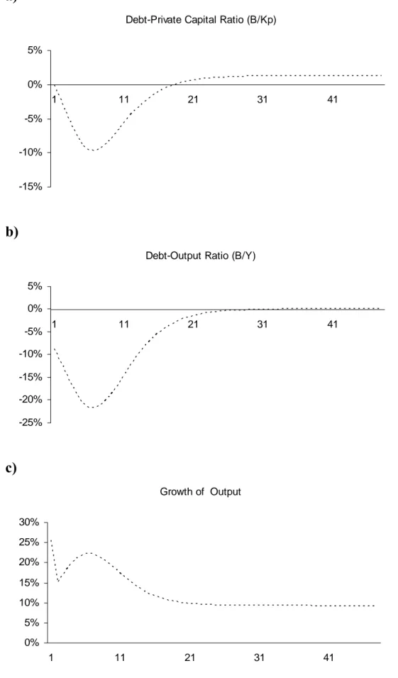
I …rst experiment with the Golden Rule, increasing the government spending shares on investment in infrastructure, and health and tracking the dynam-ics of the ratio of public debt stock to private capital, B/Kp, public debt stock to income measured as B/Y, and the growth rate of output. In or-der to do so, the baseline solution with the initial values calibrated above is …rst calculated. Then, the shock is given to the policy parameters and the model is re-simulated for t+50 periods and deviations from baseline values are obtained. As the …rst experiment, I assume that the spending share on infrastructure increases by 5 % from 0.2 to 0.2513. Figure 1 displays the de-viations from baseline values for debt private capital ratio, debt-output ratio and the growth rate of output respectively in three panels in this case.

In GR, the e¤ect of the increase in infrastructure spending on debt accu-mulation are twofold : An increase in the debt stock due to higher borrowing, and a subsequent increase in interest payments as the marginal productivity of private capital, r, also increases with the shock. The increase in interest payments translates to a higher tax base and further increases borrowing for infrastructure and crowds out private capital in subsequent periods but it also increases transfers since all government spending is proportional to the tax base. Therefore the overall e¤ect on output depends on the strength of these a¤ects and relative productivity of these factors of production.The upper and middle panels reveal that in response to an increase in vI, the

debt-output ratio drop instantenously and the magnitude of the drop gets even larger in the …rst periods. This is because public infrastructure spending is assumed to enter the production function contemporenously and output increases simultenously as vI increases but debt is a pre-determined variable

and therefore the level of debt remains constant for one period. For the same reason, debt-private capital ratio remains constant for one period after the shock, because both variables are predetermined. Apart from this, both B=Kp and B=Y display volatile dynamics, falling signi…cantly initially but stabilizing at higher values than the baseline. In essence, the debt-output ratio increases much less than debt-private capital ratio (and stabilizes at a value very close to the baseline) because the increase in vI directly e¤ects

output through infrastructure spending whereas the positive a¤ect on Kp comes through indirect a¤ects on disposable income, (1 )Y;and transfers 13_{It is essential to note that the government …nances infrastructure spending through}

as well the negative crowding out of increase in debt on private capital ac-cumulation (see 7).As the lower panel displays, the growth rate of output increases instantenously as vI increases and then displays a cyclical pattern,

increasing initially but then falling as diminishing returns set in and the inter-est rate -the return to private capital at the same time - stabilizes. However, still, there is a signi…cant increase in growth as the steady state growth rate increases by about 2%.

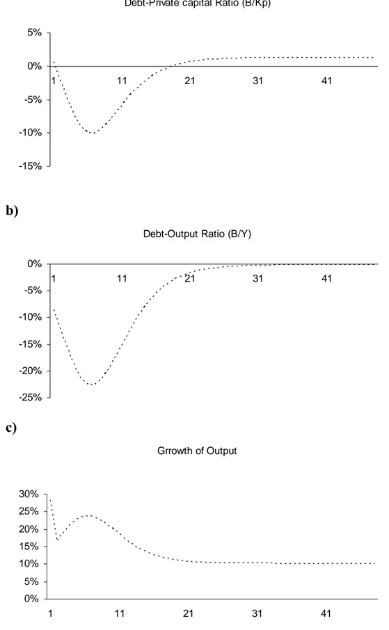
Next, consider the case that the government increases vH through

bor-rowing, althoug it is constrained by the rule to do so. In other words, let the government violate the rule permanently and increase vH by 5 per cent from

0.25 to 0.3. This experiment in a way tries to investigate the dynamics if the rule were altered and the government were allowed to borrow in order to …nance other productive spending at time 0. Figure 2 displays the dynamics in this case. The upper panel shows that public debt-private capital ratio behaves more or less similar to a increase in vI and stabilizes at a slightly

higher level than above because higher productivity of health compared to infrastructure increases the return to private capital more after the shock and the crowding out e¤ect of interest payments on transfers is higher when vH

increases by 5 per cent (see (27). Due to higher productivity of health than infrastructure, the debt-output ratio stays strictly below the baseline value, although additional spending is …nanced via borrowing. In other words, the positive a¤ect of additional health spending on output more than com-pensates for the increase in the level of debt, and therefore B=Y falls both through transition and at the steady state. Similarly, the growth rate of output is also higher than the case of an increase in vI through borrowing.

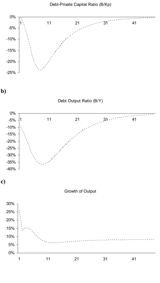
4.2.2 Primary Surplus Rule

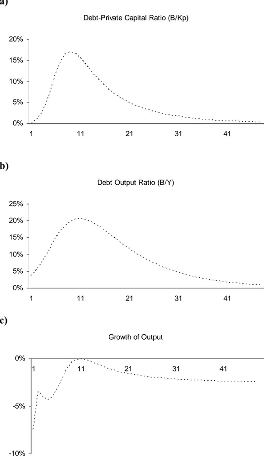
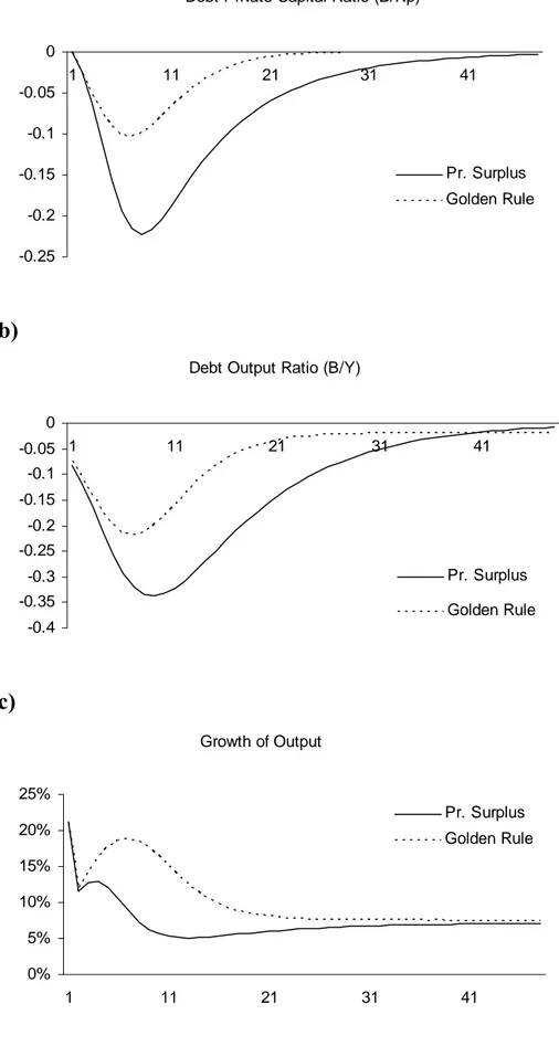
I now conduct a similar analysis using the primary surplus rule. However, in this case, since the government is only allowed to borrow for interest pay-ments, an increase in the share of infrastructure spending should be mathced with a simultenous decrease in one of the other spending shares14_{. Figure}

3 and Figure 4 display the dynamics when the 5 per cent increase in vI is

…nanced by a 5 percent decrease in share of transfers (vT)and share of health

spending (vH) respectively. When the increase in vi is …nanced by a cut in

14_{As above, it could be assumed that the rule is altered at time 0 and the government}

is allowed to borrow for productive spending here as well. However, the analysis in this paper is su¢ cient to emphasize the point so I will not pursue this way here.

vT or Vh, the behaviour of debt-private capital ratio and debt-output ra-tio entirely depends on the relative productivities of infrastructure, private capital and health. When the cut in vT …nances the additional spending on

infrastructure, the debt-private capital ratio and debt-output ratio both fall since infrastructure is calibrated to be more productive than private cap-ital with the assigned parameter values. As a result of this, the growth rate of output is also higher than the baseline value through the transition and the steady state, although the growth performance is worse than the golden rule (Figure 5). However, the opposite is true when the additional spending is …nanced by a decline in health services. Both debt-private capi-tal ratio and debt-output ratio increase and stabilize at a higher value than baseline. Further, the growth rate of output falls and stabilizes at a lower value than the baseline. Basically, this experiment, together with an in-crease in vH through borrowing under the golden rule as above, captures the

aforementioned bias towards infrastructure investment under a strict bud-getary regime. If the government is restricted to borrow for other productive spending than infrastructure as under the Golden Rule, the emphasis on infrastructure investment might lead to a lower growth and worse budget performance (measured as B=Y ) than possible through borrowing to …nance (at least partially) other productive spending, speci…ed as health here. Sim-ilarly, under a primary surplus rule where the government is not allowed to borrow to …nance any type of current or investment spending, a bias towards infrastructure might lead to a reduction on other possibly productive spend-ing, which might hamper growth and lead to a worse budget performance. In a purely growth context, this in turn requires a very careful assesment of the relative productivities of certain types of government spending.

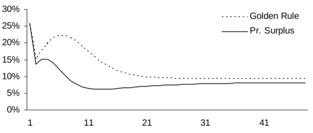
4.2.3 Cut in Unproductive Spending

Next, consider the case that the increase in infrastructure spending is …-nanced by a cut in unproductive government spending under both rules. Figure 6 compares the behaviour of variables of interest. First of all, it is clear from upper and middle panel that if we consider the debt ratios, golden rule performs much better in terms of volatility and stabilizes more quickly than primary surplus rule. The main reason for this is that the level of debt is not a¤ected by interest payments under GR and therefore the variations in interest rate is not re‡ected in the stabilization of debt-private capital and debt-output ratio. On the contrary, under the PSR, the volatility of the

interest rate also causes a large volatility in these ratios. The fall in both ratios is signi…cantly higher under the primary surplus rule than under the golden rule throughout the transition but at the steady state, they stabilize slightly below zero and very close to each other. With respect to growth, the lower panel shows that golden rule is both more stable and yields higher growth than primary surplus rule this time.

4.2.4 Increase in Tax Rate

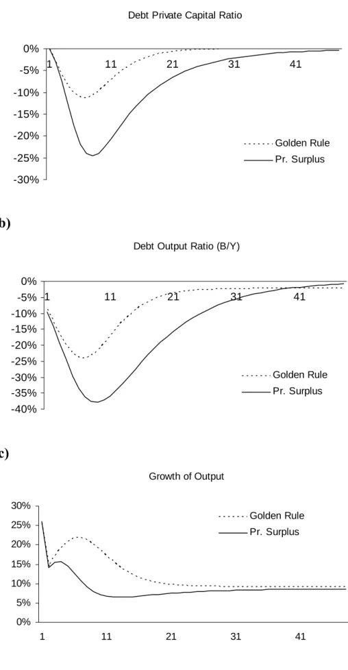
And …nally, let us assume that the government increases the tax rate by 2% from 0.2 to 0.22. This will lead to more resources from national income being spent on infrastructure and health, as well as an increase in the total level of unproductive spending and transfers and a fall in disposable income that will create a crowding out a¤ect on private capital. The results are displayed in the three panels in Figure 7. In this case, private capital ratio and debt-output ratio behave in a similar way as above. The only signi…cant di¤erence is that the Golen Rule now stabilizes at a slightly higher B=KP ratio than

the baseline, but still it is more stable than primary surplus rule. Regarding the debt-output ratio, the primary surplus rule performs better through the transition but both rules stabilize just below their baseline ratios, Golden Rule stabilizing slightly lower than its baseline compared to primary surplus rule. In terms of growth, the growth rate of output increases under both rules but Golden Rule outperforms the Primary Surplus Rule through the transition and the steady state as before.

4.2.5 Lower Health-Infrastructure Elasticity

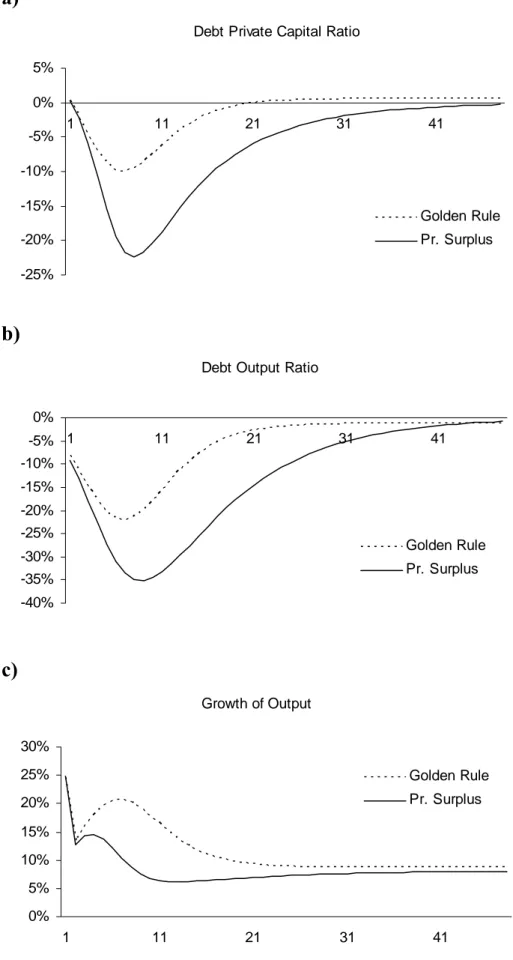
Finally, I perform experiments with the sensitivity of health output to in-frastructure capital, namely ; using the GR and Primary Surplus Rule as above and applying a 5 percentage-point increase to I …nanced by a cut in

unproductive spending. The results are displayed in Figure 8 for = 0:1. Clearly, the impact of a lower elasticity of health to infrastructure is to de-crease the fall in the debt-output ratio and debt-private capital ratio. Com-paring Figure 6 and Figure 8, it is clear that a lower elasticity of infrastructure in the production of health services favours PSR against GR. It takes the GR slightly longer now in the middle panel to catch PSR and the wedge between the growth performances of two rules is more narrow now. This is simply because with = 0:1 the government borrows for less productive

infrastruc-ture under GR and the crowding-out e¤ect of debt accumulation on private capital is thus stronger against the positive e¤ect of productive government spending on output. This result suggests that a lower elasticity of infrastruc-ture inproduction of health would strengthen the above results when the government borrows for health under the GR and invests in infrastructure through a cut in health spending under PSR. In both cases, with = 0:1; the results would favour health more against infrastructure and therefore the positive a¤ects of an increase in vH through borrowing under GR and the

negative a¤ects of increase in I through a cut in vH under PSR would simply

5

CONCLUSION

The purpose of this thesis was to examine the performance of alternative …scal rules in an endogenous growth model with public capital and debt. In order to do so, after a short introduction in the …rst chapter, the second chap-ter of the study provided a brief review of the current debate on …scal rules and the preceding endogenous growth literature that incorporates …scal rules in their analysis, as well as outlining the main economic motivation and mi-croeconomic evidence behind the analytical model. The third part presented the analytical framework, where in addition to investing in infrastructure, the government spends in health (which raises labor productivity). In turn, in-frastructure a¤ects the production of both commodities and health services. In this setting, under certain reasonable restrictions, the balanced budget rule delivers a positive growth rate and satis…es the transversality conditions but the model is also shown to be (globally) unstable under this rule. How-ever, since the case of balanced budget is far from reality for a vast majority of countries, the chapter then considers two alternative rules— a “standard” golden rule where the government is allowed to borrow for infrsatructure spending, and a “standard” primary surplus rule where the government can only borrow to …nance interest expenditures. Because the resulting models are too complex to prove stability and perform policy experiments analyti-cally (as a result of the higher dimension added by public debt accumulation and high non-linearity involved), they are compared numerically.

This was done in Chapter 3 after discussing the calibration procedures. The performances of both rules were examined in response to a variety of shocks such as an increase in the shares of spending on infrastructure and health, a reallocation of unproductive spending to infrastructure spending and an increase in the tax rate. Under a range of plausible parameter con-…gurations and spending shares, the numerical simulations showed that in response to these shocks golden rule performs better than primary surplus rule— in the sense of yielding higher steady-state growth, less volatility and more rapid convergence, despite performing slightly worse than primary sur-plus rule in terms of debt-output ratio through the transition to the new steady state. Moreover, the analysis also supported the idea that bias to-wards infrastructure could hamper growth if it leads to a decrease in other areas of potentially productive government spending such as health in this model. As was shown, borrowing for health through a modi…cation in the

rule delivers higer growth than borrowing for infrastructure under golden rule, and similarly increasing infrastructure spending through a decrease in health spending may reduce growth and increase debt-output ratio under the primary surplus rule.

One of the most importatnt policy lessons to be drawn from this analysis is that even modifying the golden ruledoes not provide a clear guide as to where one should “draw the line”on current spending. This is simply because one could always argue that education also strongly a¤ects productivity and therefore that governments should be allowed to borrow for education by the rule. The reasoning can of course be pushed further; it could be argued that wages and salaries of public servants (a large share of public spending in most countries) are “productive” to some degree because they increase the productivity of these workers and facilitate private activity. Likewise, spend-ing on defense and security, or the environment, could be viewed as bespend-ing productive— feeling safer or breathing better may lead to higher productiv-ity. Moreover, governments may have strong incentives to present various categories of spending as productive, even if the case is not clear. The im-plication therefore is that “drawing the line” becomes very di¢ cult, making the practical speci…cation of the rule extremely di¢ cult as well.

At this point, it is important to note that one further extension of this research would be to incorporate the risk premium associated with the level of public debt. This is particularly valid for developing economies that are heavily dependent on external borrowing in order to close thier savings and investment gaps. The interest rate faced by these economies includes a risk premium that increases (in general in a convex way) with the worsening of public balances over the world interest rate. Therefore, in such a setting, the deviations from baseline debt-output ratio for instance, if it is regarded as an indicator of the position of public balances, may assume great importance. As Figure 6, Figure 7 and Figure 8 show, such a speci…cation would clearly favour primary surplus rule against the golden rule, particularly through the transition process since the high negative deviations from baseline debt-output ratios would reduce the risk premium and further contribute to the improvement in public balances under the primary surplus rule. However, this would also come at a cost of even lower growth a¤ect than golden rule due to a smaller tax base to …nance productive spending. Apparently, one cannot assume a priori that the same parameter con…gurations would yield a balanced steady state growth when risk premium is accounted for. Excessive debt accumulation may always completely crowd out private investment and

there may be no balanced equilibrium for a wide range of parameters. A second important point is that as long as there exists heterogeneity among parameters and starting values, imposing uniform …scal rules “across the board” to a group of countries because they share a common mone-tary arrangement makes little sense. In countries where stocks of public in-frastructure assets are relatively low to begin with, borrowing for infrastruc-ture projects creates greater opportunity and thus makes sense— as long as the investment is su¢ ciently e¢ cient and productive. This may actually im-prove prospects for …scal stability. However, in other cases, borrowing for other forms of potentially productive government spending may prove to be more bene…cial in terms of growth. Even if the rule is slightly modi…ed to allow borrowing to partially …nance some productive current spending, the growth gains may be signi…cantly high, sometimes even higher than addi-tional spending in

infrastructure itself. This may particularly hold again for low and middle-income developing countries where the marginal product of health and edu-cation is relatively high due to low level of human and health capital accu-mulation. However, as argued above, this again brings forward the question of drawing the line on current spending.

And …nally, it must be noted that the focus on growth (and transitional dynamics) should not lead one to neglect the fact that …scal rules are also imposed in order to prevent pro-cyclical government spending from fostering macroeconomic volatility. To the extent that such volatility is detrimental to growth (as shown in a number of recent studies), a potential trade-o¤ may emerge, where if a “standard” …scal rule lowers volatility signi…cantly, constraining productive spending may ultimately prove to be bene…cial to growth. 15 _{The nature of this trade-o¤ would normally depend on a}

num-ber of institutional factors, in addition the structural characteristics of the economy. In countries where political polarization is high, or the national legislature is fragmented across a large number of political parties, for in-stance, the propensity to engage in procyclical spending may be quite strong and tight rules may be inevitable. Moreover, volatility itself may have large welfare costs, as shown by Pallage and Robe (2003), independently of its impact on growth.

15_{This volatility may particularly hamper growth through an increase in the risk}

To conclude, it is vital to emphasize that although this thesis does not provide a clear-cut answer to where one should draw the line, it clearly shows that the question of how to draw the line cannot simply be addressed by imposing well-de…ned, strict …scal regimes irrespective of each country’s pe-culiar economic and political conditions. Attempts for such simple solutions neglect the complementarities between productive government spending and private capital, as well as totally ignoring the welfare consequences of strict budgetary regimes. Therefore, a more thorough country-speci…c analysis is required to correctly identify the growth a¤ects of …scal policy and balance the trade-o¤ between growth and volatility.

Figure 1 Golden Rule- 5 % Increase in vI Through Borrowing

a)

Debt-Private Capital Ratio (B/Kp)

-15% -10% -5% 0% 5% 1 11 21 31 41

b)

Debt-Output Ratio (B/Y)

-25% -20% -15% -10% -5% 0% 5% 1 11 21 31 41

c)

Figure 2 Golden Rule- 5 % Increase in vH Through Borrowing

a)

Debt-Private capital Ratio (B/Kp)

-15% -10% -5% 0% 5% 1 11 21 31 41

b)

Debt-Output Ratio (B/Y)

-25% -20% -15% -10% -5% 0% 1 11 21 31 41

c)

Figure 3 Pr. Surplus Rule- 5 % Increase in vI Through a Cut in vT

a)

Debt-Private Capital Ratio (B/Kp)

-25% -20% -15% -10% -5% 0% 1 11 21 31 41

b)

Debt Output Ratio (B/Y)

-40% -35% -30% -25% -20% -15% -10% -5% 0% 1 11 21 31 41

c)

Figure 4: Pr Surplus Rule-5 % Increase in vI Through a Cut in vH

a)

Debt-Private Capital Ratio (B/Kp)

0% 5% 10% 15% 20% 1 11 21 31 41

b)

Debt Output Ratio (B/Y)

0% 5% 10% 15% 20% 25% 1 11 21 31 41

c)

Figure 5. 5 per cent increase in vI

Growth Rate of Output

0% 5% 10% 15% 20% 25% 30% 1 11 21 31 41 Golden Rule Pr. Surplus

Figure 6: 5% Increase in vI Through a Cut in vU

a)

Debt Private Capital Ratio

-30% -25% -20% -15% -10% -5% 0% 1 11 21 31 41 Golden Rule Pr. Surplus

b)

Debt Output Ratio (B/Y)

-40% -35% -30% -25% -20% -15% -10% -5% 0% 1 11 21 31 41 Golden Rule Pr. Surplus

c)

Figure 7: 2% Increase in Tax Rate

a)

Debt Private Capital Ratio

-25% -20% -15% -10% -5% 0% 5% 1 11 21 31 41 Golden Rule Pr. Surplus

b)

Debt Output Ratio

-40% -35% -30% -25% -20% -15% -10% -5% 0% 1 11 21 31 41 Golden Rule Pr. Surplus

c)

Figure 8: 5% Increase in vI Through a Cut in vU (μ=0.1)

a)

Debt Private Capital Ratio (B/Kp)

-0.25 -0.2 -0.15 -0.1 -0.05 0 1 11 21 31 41 Pr. Surplus Golden Rule

b)

Debt Output Ratio (B/Y)

-0.4 -0.35 -0.3 -0.25 -0.2 -0.15 -0.1 -0.05 0 1 11 21 31 41 Pr. Surplus Golden Rule

c)

REFERENCES

Agénor, Pierre-Richard, "Fiscal Policy and Endogenous Growth with Public Infrastructure," Working Paper No. 59, Centre for Growth and Business Cycle Research, University of Manchester (September 2005a).

Agénor, Pierre-Richard, "Schooling and Public Capital in a Model of Endogenous Growth," Working Paper No. 61, Centre for Growth and Business Cycle Research, University of Manchester (September 2005b).

Agénor, Pierre-Richard, "Health and Infrastructure in Models of Endogenous Growth," Working Paper No. 62, Centre for Growth and Business Cycle Research (September 2005c),

Agénor, Pierre-Richard, and Blanca Moreno-Dodson, "Public Infrastructure and Long-run Growth: New Channels and Policy Implications," unpublished, World Bank (February 2006).

Agénor, Pierre-Richard, and Kyriakos Neanidis, "The Allocation of Public

Expenditure and Long-run Growth," working paper, University of Manchester, Centre for Growth and Business cycle Research (2006).

Annichiarico, Barbara, and Nicola Giammarioli, "Fiscal Rules and Sustainability of Public Finances in an Endogenous Growth Model," Working Paper No. 381,

European Central Bank (August 2004).

Barro, Robert J., "Government Spending in a Simple Model of Endogenous Growth," Journal of Political Economy, 98 (October 1990), s103-s25.

Blanchard, Olivier J., and Francesco Giavazzi, "Improving the SGP through a Proper Accounting of Public Investment," Discussion Paper No. 4220, Centre for Economic Policy Research (February 2004).

Brauninger, Michael, "The Budget Deficit, Public Debt and Economic Growth," Journal of Public Economic Theory, 7 (December 2005), 827-.

BSB (2005) "On Economic and Social life in Turkey in Early 2005", www.bagimsizsosyalbilimciler.org

Buti, Marco, Sylvester Eijffinger, and Daniele Franco, "Revisiting the Stability and Growth Pact: Grand Design or Internal Adjustment?," Economic Paper No. 180, European Commission (January 2003).

Everaert, Gerdie, "Negative Economic Growth Externalitites from Crumbling Public Investment in Europe," unpublished, University of Ghent (July 1997).

Fair, Ray C., and John B. Taylor, "Solution and Maximum Likelihood Estimation of Dynamic Nonlinear Rational Expectations Models," Econometrica, 51 (July 1983), 1169-96.

Fernandez-Huertas, Moraga, and Jean-Pierre Vidal, "Fiscal Sustainability and Public Debt in an Endogenous Growth Model," Working Paper No. 395, European Central Bank (August 2004).

Flores, Elena, Gabriele Giudice, and Alessandro Turrini, "The Framework for Fiscal Policy in EMU: What Future after Five Years of Experience?," Economic Paper No. 223, European Commission (March 2005).

Ghosh, Sugata, and Iannis A. Mourmouras, "Endogenous Growth, Welfare and Budgetary Regimes," Journal of Macroeconomics, 26 (December 2004a), 623-35. Ghosh, Sugata, and Charles Nolan, "The Impact of Simple Fiscal Rules in Growth Models with Public Goods and Congestion," Working Paper No. 05-2, Centre for Dynamic Macroeconomic Analysis, University of Saint Andrews (January 2005).

Ghosh, Sugata, and Udayan Roy, "Fiscal Policy, Long-run Growth, and Welfare in a Stock-Flow Model of Public Goods," Canadian Journal of Economics, 37 (August 2004b), 742-56.

Greiner, Alfred, and Willi Semmler, "Endogenous Growth, Government Debt, and Budgetary Regimes," Journal of Macroeconomics, 22 (- 2000), 363-84.

Kalaitzidakis, Pantelis, and Sarantis Kalyvitis, "On the Macroeconomic

Implications of Maintenance in Public Capital," Journal of Public Economics, 88 ( 2004), 695-712.

Musgrave, Richard A., "The Nature of Budgetary Balance and the Case for a Capital Budget," American Economic Review, 29 (June 1939), 260-71.

Pallage, Stéphane, and Michel A. Robe, "On the Welfare Cost of Economic Fluctuations in Developing Countries," International Economic Review, 44 (May 2003), 677-98.

Sala-i-Martin, Xavier, Gernot Doppelhofer, and Ronald I. Miller, "Determinants of Long-Term Growth: A Bayesian Averaging of Classical Estimates (BACE)

Approach," American Economic Review, 94 (September 2004), 813-35.

Turrini, Alessandro, "Public Investment and the EU Fiscal Framework," Economic Paper No. 202, European Commission (May 2004).