C om mun.Fac.Sci.U niv.A nk.Series A 1 Volum e 66, N umb er 2, Pages 311–322 (2017) D O I: 10.1501/C om mua1_ 0000000821 ISSN 1303–5991
http://com munications.science.ankara.edu.tr/index.php?series= A 1
ESTIMATION METHODS FOR SIMPLE LINEAR REGRESSION WITH MEASUREMENT ERROR: A REAL DATA APPLICATION
RUK·IYE E. DA ¼GALP, ·IHSAN KARABULUT, AND F·IKR·I ÖZTÜRK
Abstract. The classical measurement error model is discussed in the con-text of parameter estimation of the simple linear regression. The attenuation e¤ect of measurement error on the parameter estimation is eliminated using the regression calibration and simulation extrapolation methods. The mass density of pebbles population is investigated as a real data application. The mass and volume of a pebble are regarded an error-free and error-prone vari-ables, respectively. The population mass density is considered to be the slope parameter of the simple linear regression without intercept.
1. Introduction
The classical simple linear regression model is making inferences in the functional relationship between the explanatory or independent variable X and the response or dependent variable Y from the observations (x; y): Sometimes, the explanatory variable cannot be directly observable or di¢ cult to observe for some situations. In these situations, a substitute variable W , generally called error-prone predictor, is observed instead of X that is, the random variable X is observed with measurement error U . The substitution of W for X leads to estimates that are sometimes seriously biased. The goal of the measurement error modeling is to obtain unbiased estimates with observed data (w; y).
Consider the classical linear regression model with one explanatory variable as
Y = + XX + " (1.1)
when experimental error " with mean 0, variance 2
"and the additive measurement
error model as
W = X + U (1.2)
when measurement error U with mean 0, variance 2U. When the explanatory variable is error-prone predictor the models given in (1:1) and (1:2) together is called
Received by the editors: November 08, 2016, Accepted: January 24, 2017.
2010 Mathematics Subject Classi…cation. Primary 05C38, 15A15; Secondary 05A15, 15A18. Key words and phrases. Classical measurement error model, consistent estimator, error in variables, linear regression, mass density, regression calibration, SIMEX method, M-estimation,
c 2 0 1 7 A n ka ra U n ive rsity C o m m u n ic a tio n s d e la Fa c u lté d e s S c ie n c e s d e l’U n ive rs ité d ’A n ka ra . S é rie s A 1 . M a th e m a t ic s a n d S t a tis tic s .
classical measurement error model Carroll, Ruppert, Stefanski and Crainiceanu (2006). ("; U; X) is an independent triplet with the distribution
0 @ U" X 1 A N 8 < : 0 @ 00 X 1 A ; 0 @ 2 " 0 0 0 2 U 0 0 0 2 X 1 A 9 = ; (1.3)
For the error-free data , the usual bivariate normal regression model given in (1:1) the normal estimating equations for , X and 2
" can be derived from the
condi-tional distribution of Y1; Y2; ; Yn given X1; X2; ; Xn for the random sample
(X1; Y1); (X2; Y2); ; (Xn; Yn) of size n as in Casella and Berger (1990). n X i=1 (Yi XXi) 1 Xi = 0 0 ; n X i=1 (n p) n 2 " fYi XXig2 = 0:
For error-prone data, models in (1:1) and (1:2) can be rewritten as Yi = + XXi+ "i; i = 1; 2; ; n
Wi = Xi+ Ui; i = 1; 2; ; n
for the random sample (W1; Y1); (W2; Y2); ; (Wn; Yn) of size n.
The situation is that the explanatory variable X is measured as W , i.e. ignoring the measurement error, and modeling the regression of Y on W using the model in (1:1) causes impairments of statistical inferences such as biased estimation. To be speci…c the e¤ect of the measurement error on the estimating equations is to bias on the slope estimate in the direction of 0. This type bias is commonly referred to as the attenuation in the context of the simple linear regression. The amount of the attenuation is called reliability ratio as in Fuller (1987), Carroll, Ruppert, Stefanski and Crainiceanu (2006) and denoted by .
The ordinary least squares (OLS) slope estimator ^W for the regression of Y on W is called the naive estimator and the OLS slope estimator ^X for the regression of Y on X is called the true estimator. Let us de…ne SY W, SY U and SXU are the
sample covariances of Y and W , Y and U , and X and U respectively. Similarly, SU U = SU2 and SXX = S2X the sample variances of U and X, respectively. The
ordinary least square estimator on the observed data (Y; W ) is written as ^W = ^ ^
X+ op(1), where the estimator of the reliability ratio is ^ = SX2=(S2X+ SU2) and
op(1) indicates that the remainder term converges in probability to zero. In order
to show that …rstly, consider the naive ordinary least square estimator of slope parameter as ^ W = SY W SW W = SY X + SY U SXX+ SU U :
Secondly, by the Law of Large numbers, SXU and SY U converge in probability to
zero under the independence assumption, and likewise SXX p ! 2 X, SU U p ! 2 U, SY X p
! Y X as n ! 1. From these results, ^ ! = 2X=( 2X+ 2U) as n ! 1
and the regression slope parameter is X = Y X= 2X, therefore ^W p
! X as
n ! 1 (Ser‡ing, 1980). The attenuation factor is a real number in the range [0,1] since 2
X, 2U are …nite. If 2X > 0 and …nite, then 2U = 0 , = 1. In this
situation, there is no measurement error, say, X = W . If 2
U = 1 , = 0, then
the data is all error.
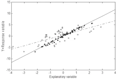
To illustrate the attenuation induced by the measurement error, the data for the true explanatory variable X, the regression model error ", and the measurement error U were generated from the trivariate normal distribution as
X; U; " T N 0; 0; 0 T; diag f1; 0:5; 0:5g :
The data for the response variable Y were generated with the regression model, Y = + XX + " with = 0, X = 3 and the observed data W were obtained
from W = X + U . Notice that how to the true data (Xi; Yi)’s are more tightly
grouped around a well-delineated line, while the error-prone data (Wi; Yi) have
much variability about the dashed line in Figure 1.
Figure 1. Illustration of the simple linear regression with mea-surement error. The …lled circles are the plot of the true data (X; Y ), and the dashed line is the least squares …t of these data. The empty circles are the plot of the observed data (W; Y ) and the solid line, which is the attenuated line, is the least squares …t of the measurement error data. For these data 2
X = 1, 2U = 2" = 0:5
The results of …tting the model with measurement error can be summarized roughly as fallows. The regression model for E(Y jX) depends on unobservable explanatory variable X instead of observable substitute variable W to X. As a consequence, the estimators of the parameters of interest = ( ; X)T appear in the the model are functions of the observed substitute variable W . The data have also additional variability because of the measurement error. Thus, it is di¢ cult to …nd unbiased estimator of the parameters of interest with the substitute variable W instead of X. On the other hand, one of the feature of the measurement model has a lack of identi…ability problem (Fuller (1987), pp. 9-10). Because, the estimation of measurement error variance, ^2U, can not be obtained with the data (W; Y ) at hand, so for this estimation it is required replicated data unless it is known. As a results, not only is the regression slope estimator biased and the …tted line attenuated, but also the data are noisier with increased error about the …tted line. In this manuscript, two methods of correcting the attenuation, the regression calibration and simulation of extrapolation called SIMEX, are explained in more detail and compared in terms of the attenuation and variability. For the illustration a simulation study is presented for di¤erent sample sizes and di¤erent values of
2
U; 2". Moreover, a real data example is given for an application to linear regression
without intercept.
2. The Methods of Estimates
2.1. Regression Calibration. The regression calibration (RC) is a straightfor-ward method for …tting the regression models in the presence of measurement error and was derived and recommended by Carroll and Stefanski (1990) and Gleser (1990). The RC is one of the most useful methods to reduce the e¤ect of measure-ment error and correcting the attenuation in regression model. The basis of RC is the replacement of the true explanatory variable X by the estimation of E(XjW ), which is denoted as E(XjW ) and also will be called as RC function. After this\ replacement, the regression analysis is performed on E(XjW ); Y . RC is simple,\ widely used, e¤ective, reasonably well investigated and potentially applicable in addition to correcting the attenuation (Carroll and Stefanski (1990, 1994)).
Carroll and Stefanski (1990) suggested an algorithm yielding a linear approxima-tion to the RC estimate to eliminate bias in the estimated regression coe¢ cients for measurement error analysis. To operate the algorithm, measurement error variance
2
U has to be known or estimable. If the data are replicated externally or internally
to estimate the error variance, then the algorithm is applicable. RC estimate of X can be derived in two steps:
The mean squares of model error (MSE) for …tting the regression Y on W is taken ^2W. If there is only one explanatory variable in the analysis like this article, ^2W is the sample variance of W .
With the replicated data, it is possible to estimate the measurement error vari-ance 2
U. Replicate data means that measurement of X is replicated measurements
W measuring the same X. Suppose Wi1; Wi2; : : : ; Wiki are ki replicated
measure-ments of Xi, and their mean is Wi:. The replication provides to obtain the estimate
of measurement error variance as
b2U = n P i=1 ki P j=1 (Wij Wi:)2 n P i=1 (ki 1) : (2.1)
Given W , the best linear approximation to X is E(X W ) X+ 2X 2X+ 2U =k
1
W W ;
where k is the number of the replication of X, X and W are the means of X and W , 2
X and 2U are the covariance matrices of X and U , respectively (Carroll,
Ruppert, Stefanski and Crainiceanu (2006)).
For the RC estimate, the sample mean of the replicated data of Xi is Wi: = ki
P
j=1
Wij=ki and the pooled sample variance of the replicated data is given in (2:1).
Similarly, the other estimates are de…ned as
bX =bX = n P i=1 kiWi: n P i=1 ki , v = n X i=1 ki n P i=1 k2 i n P i=1 ki ; b2X= "( n X i=1 ki Wi: bW 2 ) (n 1)b2U # =v: resulting RC estimate is b Xi=E(X\i Wi:) ^W +b 2 X " b2X+b 2 U ki # 1 Wi: ^W , i = 1; 2; : : : ; n: (2.2)
The estimated RC in (2:2) is reproduced by replacing the unknown parameters by their classical method of moments estimators in the best linear approximation to X given above. To derive RC estimate it is required to have the estimatesb2U and
b2W from observed data. If the data are not replicated or unavailable to replicate,
and but there is an estimate 2
U, gotten from an another study, still the estimate
b
Xi can be obtained from equation (2:2). Even if there are exactly two replicates of
W , then the sample variance of U is derived from the half of the sample variance of di¤erence Wi1 Wi2. Thus, the estimated RC is attained as in (2:1). When the
estimate of variance 2
U is derived from replicated data, the covariance "U of " and
U is assumed to be zero since the independence of " and U . When the replication is not available for each observation, the algorithm for RC estimator produces consistent estimates for linear regression. After reducing the measurement error in the explanatory variable, then the regression parameters are estimated and the statistical inference proceeds with a standard analysis. SIMEX, given in the next section has the same advantages with RC, but it is more computationally intensive than RC.
2.2. Simulation Extrapolation. Simulation Extrapolation (SIMEX) is a sim-ulation based method of estimating and correcting the attenuation due to the measurement error. SIMEX method was proposed and developed by Cook and Stefanski (1994), Stefanski and Cook (1995) as an alternative method to reducing bias. SIMEX estimation is a computational, graphical method and depends on a computer algorithm that determines parameter estimates.The essential idea is to determine the bias for an estimate caused by the measurement error by implement-ing a virtual experiment via simulation then the unbiased estimation is found on the graph for the no measurement error case.
SIMEX estimates are obtained by adding additional measurement errors to the observed values of the explanatory variable W in a resampling-like stage and re-calculating the naive estimators from the contaminated data. For each additional measurement error, the naive estimator is obtained and the trend is then extrapo-lated back to the case of no measurement error. The details of the algorithm are given in this section for simple linear regression.
The key features of SIMEX method are described easily for the simple linear regression. For this, the notation is adopted from Carroll, Ruppert, Stefanski and Crainiceanu (2006). Suppose that simple linear regression Y = + xX + ", with additive measurement error model W = X + U , where U is independent of (Y; X) and has mean zero and variance 2
U. For the calculation purpose, assume
U = UZ, where Z is a standard normal random variable. 2Xdenotes the variance
of the explanatory variable X, the measurement error variance 2
U assumed to
be known or to be estimated. Let now the additive measurement error model be W = X + UZ. When the measurement error variance is ignored, it is well known
that the ordinary least square estimate ^W, denotes the naive estimator, of X converges in probability to 2 X 2 X+ 2U X as n ! 1, but not to X.
The key idea of SIMEX method is to obtain the ordinary least square estimate of slope from the original data that is the naive estimate ^W. There are M 1 additional data sets with successively added measurement error that each set has the variance 2
U(1 + m), m = 1; 2; ; M where 0 = 1< 2< < M. In the
following the set of ms is denoted by . For any mth data set, the ordinary least
2 X
( 2
X+ (1 + ) 2U)
X. Note that, for = 1 the naive estimator turns out to be
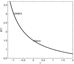
an unbiased estimator of X. This suggest that the relationship between ^W and can be formulated as a nonlinear regression model. Therefore, is taken as if an independent variable and ^W is taken as if a dependent variable. The model has a mean function of the form
E(^Wj ) = g( ) = 2 X 2 X+ 2U(1 + ) X ; > 0: (2.3)
A generic plot of versus g( ) is obtained as in Figure 2. The parameter of interest, X is achieved from the function g( ) by extrapolation to = 1 (Carroll, Ruppert, Stefanski and Crainiceanu (2006)). Cook and Stefanski (1994)
Figure 2. A generic SIMEX plot of the e¤ect of measurement error of size 2
U(1 + ) on parameter estimates. The SIMEX
esti-mate is an extrapolation to = 1 and the naive estimate occurs at = 0.
showed that equation (2:3) …ts the nonlinear function g( ) = 0+ 1( 2+ ) 1 of
named as the rational linear extrapolant that generates consistent estimator of the parameter of interest. For the unbiased parameter estimation let us recall a commonly used M-estimation method via score function which satis…es the
E [ (Y; X; ) jX ] = 0
where Y = g( ), X = and = ( 0; 1; 2)T are considered as response,
explana-tory variables and the vector of parameters, respectively.
The conditionally unbiased function can be devised using the M-estimation methods described by Carroll, Ruppert, Stefanski and Crainiceanu (2006, Sec.7.3).
The parameter relating Y and X is consistently estimated by ^ satisfying the estimating equation n X i=1 (Yi; Xi; ) = 0: (2.4)
The SIMEX algorithm suggested by Cook and Stefanski (1994) can be summa-rized in the following steps:
Fix the set and choose m2 .
Take a constant B > 0 and generally considered as B = 50; 100; 500. Generate the random variables Zib N (0; 1) via computer for b = 1; ; B
and i = 1; ; n.
De…ne the variance V ar(Wi+ U 1=2m ZibjXi) = (1 + m) 2U; i = 1; ; n.
De…ne the estimate ^b( m) be a solution of n
P
i=1
(Yi; Wi+ U 1=2m Zib; ) = 0
for each b.
Average these estimations as ^ S( m) = 1 B B X b=1 ^ b( m);
where the subscript S refers to the simulation nature of the estimator. Repeat the steps for m = 1; 2; ; M and …nd ^S( m) for each m.
Plot the generated data of pairs ( m; ^S( m)).
Fit the parametric model g( ; ) = 0+ 1( 2+ ) 1 by ( m; ^S( m)) and
estimate = ( 0; 1; 2) T
.
Find the SIMEX estimator as ^SIM EX = g(^; 1)
When = 0, the SIMEX algorithm produces the estimator ^S(0), which denotes
the naive estimator the same as the method of moments estimator. The estimating equation in (2:4) satis…es E h Y; W + U 1=2Z; i = 0:
Therefore, the parameter estimator ^S( ) converges in probability to ( ) by the
standard estimating equation theory (Ser‡ing, 1980). 3. Simulation Study
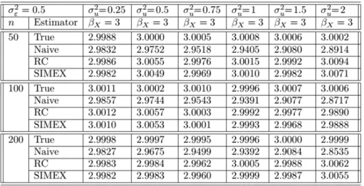
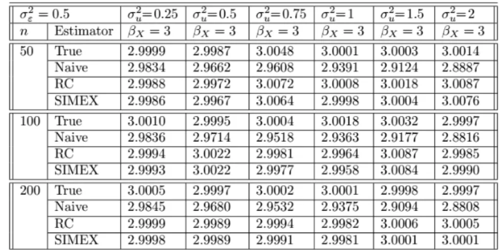
In this section, the performance of regression calibration and SIMEX methods are illustrated by a simulation study to eliminate the e¤ects of measurement error on the parameter estimation. Throughout the simulation study measurement error variance, 2
U is assumed to be known. The data fXi; Ui; "igni=1 are generated from
trivariate normal distribution as in (1:3) with X = 0 and 2
X= 1 for the selected
the measurement error variances 2
U = f0:25; 0:5; 0:75; 1:0; 1:5; 2:0g, the model error
variances 2
runs. The data for the response variable Y and the observed variable W were created by using the generated data for the models given in (1:1),(1:2) with = 0,
X = 3. The simulation results are given only for the estimated parameter X in
Table 1 and Table 2. The slope estimations depending on the methods are listed below with the associated data:
True estimation calculated from the true data fYi; Xigni=1,
Naive estimation calculated from the observed data fYi; Wigni=1,
RC estimation calculated from the observed data fYi; Wigni=1,
SIMEX estimation calculated from the observed data fYi; Wigni=1:
Table 1. Simulation study results for the true, naive, RC and SIMEX estimators for 2U = f0:25; 0:5; 0:75; 1:0; 1:5; 2:0g ; 2"= 0:5;
n = f50; 100; 200g ; and ( ; X) = f0; 3g :
Table 2. Simulation study results for the true, naive, RC and SIMEX estimators for 2
U = f0:25; 0:5; 0:75; 1:0; 1:5; 2:0g ; 2"= 1; n = f50; 100; 200g ;
and ( ; X) = f0; 3g : The table entries are means of 100 simulation runs.
The true, naive, RC and SIMEX estimations were compared in terms of bias. As seen in tables, RC and SIMEX methods eliminate the attenuation due to mea-surement error. That means, both methods correct the bias of the estimates of regression parameters as well as true estimation. When the sample size increases, SIMEX method gives slightly better estimates than RC.
4. An Application
The interest is to …nd the density of pebble population in one of the coasts of Antalya. Pebbles are di¤erent colors (granite or white, etc.) which re‡ect their texture and density. For the application purpose the sample pebbles are randomly selected from the population of pebbles which have the same color and texture, namely granite colored. So, the density of a granite pebble can be obtained as
=m
V ) m = V
where =density, V =volume(cm3) and m= mass(g). The volume and mass of each pebble are measured with measuring cylinder and a very sensitive weight scale, and then their densities can be obtained from the density formula given above. However, the volume of a pebble is not easily measured even though it is measured with a very sensitive instrument. The volume measurement can be considered as an error-prone variable; therefore it is possible to be modeled as in (1:2). Throughout the application the volume of the pebbles are assumed to be never measured accurately. On the other hand the population density can be estimated as a slope parameter of a simple linear regression model without intercept.
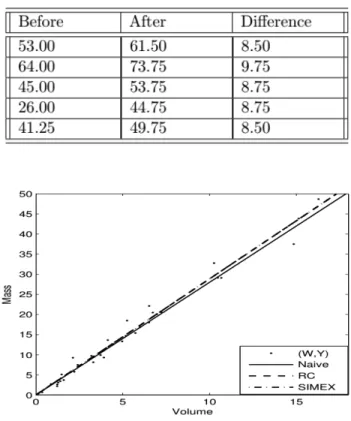
For the analysis purposes, suppose that the measurement error of volume is U N (0; 2
a replicated sample. For this aim, a metal sphere with known volume V = 9:20 cm3
is measured several times to calculate the measurement error variance using this replicated data given in Table 3. For this data the measuring cylinder …lled with water randomly and measured the level of the water referred as "Before" then the metal sphere put inside the measuring cylinder and measured the level of the water referred as "After". The di¤erence After and Before denotes the volume of the metal sphere for each measurement replication. Note that the each value of "Di¤erence" varies even if it is measured the same metal sphere which indicates that volume measurand has a measurement error.
Table 3. Measurements of a sphere has volume 9.20 cm3,
measured with a measuring cylinder.
Figure 3. The estimated regression lines of the pebbles data for naive, RC and SIMEX estimator
From the replicated data given in Table 3, the measurement error variance 2 U
is estimated as 0:52. The volume and the mass of pebbles are called as W = V and Y = m, respectively to be compatible with the models (1:1) and (1:2). To …t the data, the simple linear regression model and the additive measurement error model
are
Yi = Xi+ "i; i = 1; 2; : : : ; 38
Wi = Xi+ Ui; i = 1; 2; : : : ; 38
The estimated regression lines using the pebbles data are ^yi= 2:8575wiwith the
OLS estimator, ^yi = 2:8868wi with the RC estimator and ^yi = 2:8869wi with the
SIMEX estimator.
The three estimated regression lines of OLS, RC and SIMEX appear to be very close in Figure 3. The slope estimations of RC and SIMEX produce relatively close to each other than the OLS. There are some possible reasons for indistinctiveness of the estimated lines such as small measurement error variance, small pebble sizes, small sample size etc. The estimated reliability ratio is ^ = 0:9898 for the current application. It seems that the e¤ect of measurement error will be more apparent as the pebble sizes increase.
References
[1] Carroll, R.J & Stefanski, L.A. , Approximate quasilikelihood estimation in models with sur-rogate predictors, Journal of the American Statistical Association, (1990), 85, pp. 652-663. [2] Carroll, R.J., Ruppert, D., Stefanski, L.A.& Crainiceanu, C.M., Measurement Error in
Non-linear Models, 2nd edn.Chapman & Hall/CRC 2006.
[3] Casella, G. & Berger, R. L. Statistical Inference, Duxbury Press, Belmont, 1990.
[4] Cook, J.R. & Stefanski, L.A., Simulation Extrapolation Estimation in Parametric Measure-ment Error Models, Journal of the American Statistical Association, (1994), 89, pp. 1314-1328. [5] Fuller, W.A., Measurement Error Models, John Wiley and Sons, New York, 1987.
[6] Gleser, L.J., Improvements of the naive approach to estimation in nonlinear errors-in-variables regression models. In Statistical Analysis of Error Measurement Models and Application, P. J. Brown and W. A. Fuller, ed., Providence: American Mathematics Society, 1990.
[7] Ser‡ing, R.J., Approximation Theorems of Mathematical Statistics, John Wiley and Sons, Singapore, 1980.
[8] Stefanski, L.A. & Cook, J.R., Simulation-Extrapolation: The Measurement Error, Journal of the American Statistical Association, (1995), 90, pp. 1247-1256.
Current address : Rukiye E. Da¼galp (Corresponding author): Ankara University, Faculty of Sciences, Department of Statistics, 06100 Tando¼gan-Ankara/Turkey.
E-mail address : [email protected]
Current address : ·Ihsan Karabulut:Ankara University, Faculty of Sciences, Department of Sta-tistics, 06100 Tando¼gan-Ankara/Turkey.
E-mail address : [email protected]
Current address : Fikri Öztürk:Ankara University, Faculty of Sciences, Department of Statis-tics, 06100 Tando¼gan-Ankara/Turkey.