The Investigation of Relationship between Solar Parameters and Total Electron Content over Mid-Latitude Ionosphere

The Investigation of Relationship between Solar Parameters and Total

Electron Content over Mid-Latitude Ionosphere

Ramazan Atıcı 1*, Selçuk Sağır2

1Muş Alparslan University, Faculty of Education, Department of Classroom Teaching, Muş, Turkey,

+904362494949, [email protected]

2 _{Mus Alparslan University, Department of Electronics and Otomation, Vocational School, Mus, Turkey,}

+904362494949, [email protected] *Corresponding author Received: 8 January 2017 Accepted: 10 July 2017 DOI: 10.18466/cbayarfbe.339346 Abstract

In this study, the relationship with solar parameters (F10.7 index, proton density and proton speed) of the Total Electron Content (TEC) values obtained from IONOLAB and IRI-2012 models is statistically examined during equinox months (March and September) of 2009 over mid-latitude ionosphere for night and day time. As a statistical tool, a multiple regression model is used to determine the relationship between solar parameters and TEC values. At Universal Time (UT) 1200, the explainable rates by solar parameters of TEC changes are calculated as 58% and 55% for IONOLAB TEC values in March and September equinox months, on the other hand these rates are obtained as 99% and 57% for IRI-2012 TEC values. At 2400UT, 57 % and 39 % of changes in IONOLAB and 51 % and 59 % of changes in IRI-2012 TEC values during equinox months could be explainable by solar parameters, respectively. It is observed that the TEC values are higher than IRI-2012 TEC values on both equinox months. Also, IONOLAB-TEC values on September 2009 are greater than ones on March 2009. When compared to the two models, we concluded that IONOLAB model is more sensitive than IRI-2012 model to the changes occurring in the sun over mid-latitude.

Key words: IRI-2012, IONOLAB, Mid-Latitude Ionosphere, Solar Parameters, TEC

1. Introduction

Solar radiation penetrated the Earth’s upper atmosphere leads to heating, dissociation and ionization by absorbing via particles in the medium, and thus the ionosphere is primarily formed via the ionization effect of solar extra ultraviolet (EUV). The features of the ionosphere change importantly during solar activity events and they may have critical conclusions on the geospace environment (e.g. geomagnetic storms, ionospheric and thermospheric storms). Enormous variations in the neutral density and temperature, ion and electron densities and temperatures, neutral winds, and electric fields in the ionosphere are initiated by the variability of the solar activity [1-3]. The key parameter of ionosphere is the electron density and needed information to study the ionospheric variability is provided by its distribution in space and time [4, 5]. Since the direct measurement of electron density of ionosphere is not possible, it is usually conducted by ionosondes, incoherent scatter radars, ground-based transmitters and satellites, but these measurement methods are both spatially and temporally scarce and expensive [5, 6]. Recently, the Global Positioning System (GPS) signals present a chance for

ionospheric investigation. For the study of the ionosphere, GPS data are used commonly in many research studies [7-12].

The distribution and characteristics of TEC over low, mid, and high latitudes have been investigated by several researchers [11, 13-20]. Because of measurements of TEC by using GPS data are not possible over all places, some models carried out to understand the global distribution of TEC by different researchers. The globally used models for ionospheric TEC measurements are the International Reference Ionosphere (IRI) [21, 22], semi-empirical low-latitude ionospheric model (SLIM) [23], parameterized, real-time ionospheric specification model (PRISM) [24], NeQuick-2 [25], Utah State University-Global Assimilation of Ionospheric Measurements (USA-GAIM) [26] and Ionosphere Research Laboratory (IONOLAB) TEC model that carried out IONOLAB-group [12, 27-28]. The IRI model is commonly used by ionospheric researchers. At present time, the IRI-2012 is the most recent version of this model [29]. A brief review about GPS-based ionospheric modeling is presented by [30, 31].

In this study, the relationship between solar parameters and IONOLAB-TEC and IRI-2012 models is investigated during equinox months of 2009, when it has a deep minimum. The main aims of this study are to investigate the relationship between TEC-values and solar parameters and to compare the sensitivity of IRI-2012 and IONOLAB-TEC models in terms of the changes occurred on the sun at mid-latitude region. The data from IONOLAB and IRI-2012 models are obtained from Ankara GPS station in Turkey located at mid-latitude ionosphere for universal time (UT) 12:00 and 24:00. Then, the relationship between solar parameters (proton speed, proton density and F10.7 flux) and TEC values is statistically investigated.

2. Statistical analysis method

In the present study, the multiple regression analysis method is used to reveal the relationship between dependent (TEC values) and independent (solar parameters) variables. The multiple regression analysis consists of three stages; namely, unit root test, co-integration test and regression model. The unit root test is used to investigate whether the variables is stationary or not. If the variables are stationary, then co-integration test is applied to determine whether a long-term relationship between the variables exists or not. After this stage, the regression equation sets up between the variables and it is investigated how the variables are connected to each other [32-34].

Model used in this study is the same as references [33-36]. For more information about the model see these references [33-36]. The equation including the lagged values of the dependent variable is defined by adding a constant and a time trend as follows [32-34];

t k j j t j t t

t

δy

α

y

ε

Δy

=

+

+

+

∑

+

= − − 1 1

Δ

β

μ

(1)

Where

y

is the dependent variable,

μ

is the mean value,

β

is the coefficient of time trend,

Δ

is the difference

processor, t is the time trend,

ε

is the error term, and k

is the number of lags. After the stability of variables and existence of the long-term stability between the variables have been determined, the requiring equations are derived from Eq. (1), depending on the stability of the variables.

3. Results and Discussions

To investigate the relationship between the variables, TEC values for coordinates (39.7 N; 32.76 E) of Ankara, Turkey at universal time (UT) 12:00 and 24:00 during equinox months of 2009 are taken from IONOLAB

website (www.ionolab.org) and IRI-2012 website

(http://omniweb.gsfc.nasa.gov/vitmo/iri2012_vitmo.htm

l).

Similarly for the same station; values of solar parameters (proton density, proton speed and F10.7 flux) are taken from OMNIWeb Data Explorer website

(http://omniweb.gsfc.nasa.gov/form/dx1.html).

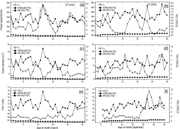
3.

Results obtained for the universal time 12:00

Figure 1 demonstrates the relationship with solar parameters of TEC values obtained from IONOLAB and IRI-2012 models for 12:00 UT during equinox months of 2009, when it is having a deep minimum. (a), (c) and (e) panels determine the relationship with IONOLAB-TEC (or GPS-TEC) and IRI-2012-TEC values of proton speed

(

V

_p

), proton density (

N

_p

) and

F10.7

solar flux in

March equinox of 2009, respectively. When the proton speed and density are investigated the relationship with TEC values, it is observed that GPS-TEC values are

directly proportional with

V

_p

and

N

_p

almost the whole

month. However, IRI-2012-TEC values increase linearly

during the entire month. While the

F10.7

cm solar flux

values vary directly proportional with GPS-TEC values on 01-06 March and 18-30 March, it vary inversely proportional on 6-18 March. It could be concluded that IRI-2012-TEC values over especially Turkey obtained for mid-latitude coordinates are not sensitive in terms of variations occurred in solar parameters.

(b), (d) and (f) panels illustrate the relationship with IONOLAB-TEC and IRI-2012-TEC values of proton

speed (

V

_p

), proton density (

N

_p

) and

F10.7

solar flux

in September equinox of 2009, respectively. It is seen that the relationship with proton speed of GPS-TEC values is directly proportional during entire month, except for 07-14 September. When the relationship between proton density and GPS-TEC values is investigated, it is seen that the variation of GPS-TEC values with proton density is proportional between 01-07 September and 19-25 September while in other days are inversely proportional. It is observed that the change of F10.7 cm solar flux with GPS-TEC values is in direct proportional after on 20 September, while it is not distinct relationship between the variables before on 20 September. However, there is no relationship between IRI-2012 TEC and solar parameters during whole month as in March equinox and the IRI-2012-TEC values increase linearly. Morover, it is seen that the GPS-TEC values are greater in September than in March at 12:00 UT. Since GPS-TEC values calculate as total electron content in column up to satellite height (20.200 km), it is always greater than IRI-2012-TEC values. In a previous study [37], it is expressed that IRI-TEC values are less than GPS-TEC values for both March and September equinox at 12UT in a station located at European mid-latitude. This result is compatible with the result obtained here. In addition, in another study [38] it is explained that IRI-TEC values are less than GPS-TEC values at noon during March equinox. .

6 12 18 24 30 280 320 360 400 440 480 520 560 P rot an s peed ( k m /s ) 9 10 11 12 13 14 15 16 17 18 19 0 5 10 15 20 25 30 280 320 360 400 440 480 520 560 v_p IONOLAB-TEC IRI-2012-TEC Np IONOLAB-TEC IRI-2012-TEC 10 11 12 13 14 15 16 17 18 19 (f) (e) (c) (b) T E C ( T E CU) (a) 6 12 18 24 30 4 8 12 16 20 P rot on dens it y ( c m -3) UT 12:00 10 12 14 16 18 20 6 12 18 24 30 0 4 8 12 16 20 (d) N_p IONOLAB-TEC IRI-2012-TEC F10.7 IONOLAB-TEC IRI-2012-TEC 10 12 14 16 18 T E C ( T E CU) 6 12 18 24 30 67 68 69 70 71 72 73 74 75 76 77

days of month (march)

F 10. 7 ( s fu) 9 10 11 12 13 14 15 16 17 18 19 UT 12:00 v_p IONOLAB-TEC IRI-2012-TEC 6 12 18 24 30 69 70 71 72 73 74 75 76 77 _F10.7 IONOLAB-TEC IRI-2012-TEC

days of month (september)

10 11 12 13 14 15 16 17 18 19 T E C ( T E CU)

Figure 1 The variation of total electron content at mid-latitude region depending on solar parameters for UT 12:00

during March (left panel) and September (right panel) equinox months of 2009 year. However, in the September equinox, the researchers

indicate that IRI-TEC values have a combination of both over and underestimations from sunset to sunrise and noontime, respectively. Moreover, the authors of reference [39] state that the IRI-model tends to underestimate the TEC values in the day time hour (1200-1800 LT) during equinox in their study.

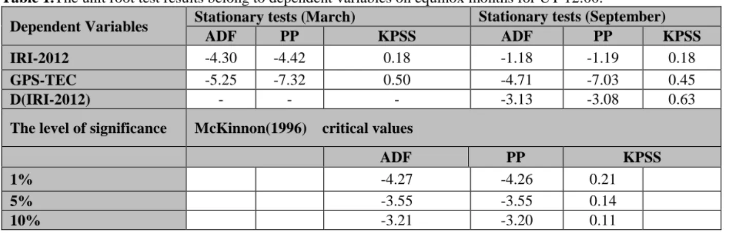
Table 1 illustrates the unit root test results of dependent variables (GPS-TEC and IRI-2012-TEC) on March and September equinox months of 2009 year. As the condition of stationarity, it is required that all test (the

Augmented-Dickey Fuller Test (ADF), Phillips-Perron

Test (PP), and Kwiatkowski-Phillips-Schmidt-Shin Test (KPSS)) results of GPS-TEC and IRI-2012-TEC variables indicated in the top row of the table are needed to be greater than McKinnon [40] critical values, which given in the bottom row of the table. GPS-TEC and IRI-2012-TEC values are stationarity in March and September except for IRI-2012-TEC values in September. To make the IRI-2012-TEC in September is stationarity; it is required to take first difference of this variable.

Table 1.The unit root test results belong to dependent variables on equinox months for UT 12:00.

Dependent Variables Stationary tests (March) Stationary tests (September)

ADF PP KPSS ADF PP KPSS

IRI-2012 -4.30 -4.42 0.18 -1.18 -1.19 0.18

GPS-TEC -5.25 -7.32 0.50 -4.71 -7.03 0.45

D(IRI-2012) - - - -3.13 -3.08 0.63

The level of significance McKinnon(1996) critical values

ADF PP KPSS

1% -4.27 -4.26 0.21

5% -3.55 -3.55 0.14

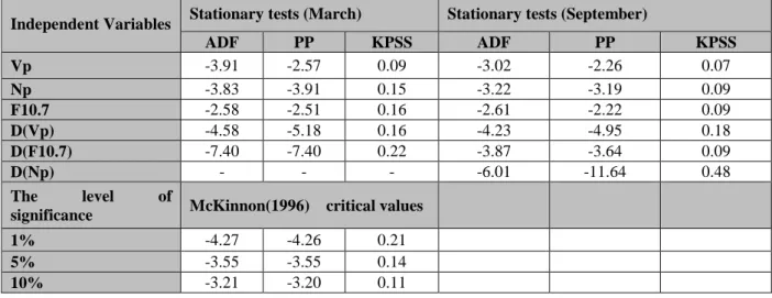
Table 2 demonstrates the unit root test results of

independent variables (

V

_p

,

N

_p

and F10.7) on March

and September equinox months of 2009. It is observed

that the all variables are not stationarity except for

N

_p

variables in March. The variables (D(

V

_p

), D(

N

_p

) and

D(F10.7) ) are made stationary by taking their first differences.

The stage after determining stationarity of dependent and independent variables, it is identified whether there is a long-term relationship between the variables or not. This

process is conducted by co-integration test. The presence of long-term relationship between the variables according to the setup models (eq. (2 and 3)) for the dependent variables is given at Table 3. To be a long-term relationship between the variables, it is required that the ADF values of the models are greater than McKinnon critical values in absolute value and the p-value is smaller than 0.05. Thus, it could be concluded that there is a long-term relationship between the variables. After determining the stationarity of variables and detecting there is a long-term relationship between the variables, the following equations are derived by eq. (1) depending on stationarity of the variables:

Table 2. The unit root test results belong to independent variables for equinox months.

Independent Variables Stationary tests (March) Stationary tests (September)

ADF PP KPSS ADF PP KPSS Vp -3.91 -2.57 0.09 -3.02 -2.26 0.07 Np -3.83 -3.91 0.15 -3.22 -3.19 0.09 F10.7 -2.58 -2.51 0.16 -2.61 -2.22 0.09 D(Vp) -4.58 -5.18 0.16 -4.23 -4.95 0.18 D(F10.7) -7.40 -7.40 0.22 -3.87 -3.64 0.09 D(Np) - - - -6.01 -11.64 0.48 The level of

significance McKinnon(1996) critical values

1% -4.27 -4.26 0.21

5% -3.55 -3.55 0.14

10% -3.21 -3.20 0.11

Table 3. The co-integration test results for IRI-2012 and GPS-TEC values on equinox months at 12:00 UT.

Regression Model March equinox September equinox

ADF p-value ADF p-value

Model (IRI-2012) -4.81 0.000 -5.60 0.000

Model (GPS-TEC) -4.74 0.000 -5.39 0.000 0.000

The level of significance McKinnon(1996) critical values

1% -2.65 5% -1.95 10% -1.60 For IRI-2012-TEC; ε D(F10.7) 2 β ) P (N 1 β )) P (D(V 0 β c 1200 TEC) (IRI + + + + = − (2) For GPS-TEC; ε D(F10.7) 2 β ) P (N 1 β )) P (D(V 0 β c 1200 TEC) (GPS + + + + = − (3) where c is constant, s

β is coefficient of variables and ε

is error term. The results at Table 5 are obtained by established models.

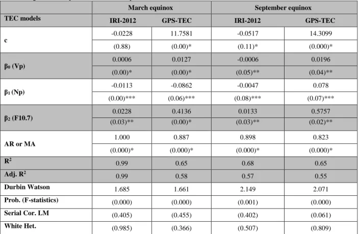
Since the values given in the four lines at the bottom of the Table 4 provide the reference values of the relevant statistical test, these values support the accuracy of the regression models in a statistical manner. These reference values given as: White Heteroskedasticity (White Het.) and Serial Cor. LM tests values must be larger than 0.05. The Durbin-Watson test values need to be between 1.5

and 2.5. Probability (F-statistics) (Prob. (F-statistic)) test values must be also smaller than 0.05 [see, 32, 33]. When the results obtained from IRI-2012-TEC dependent variable are investigated, it is observed that

the variation in

V

_p

of 1 km/s leads to an increase of 6

×

1012 _e/m2 _{in IRI-2012-TEC values in March. Similarly,}

the variation of 1 unit at F10.7 cm flux gives rise to an

increase of 228

×

1012_e/m2 _{in IRI-2012-TEC values.}

However, the variation of 1 N/cm3 _in

p

N

causes a

decrease of 113

×

1012 _e/m2 _{in IRI-2012-TEC values.}

Thus, F10.7 cm solar flux has the greatest effect on

IRI-2012-TEC values, whereas

V

_p

has the smallest effect on

it. Adj. R2 _{value, that expressed as explainable rate by}

independent variables of dependent variable for multiple relationship, is rate of 99 % and this rate is very high. In previous studies that investigated the relation between the F10.7 and foF2, in the study of reference [41]

reported a value of r=0.99 in Rome and Slough stations, and the researchers of reference [42] emphasized a strong relation between TEC and F10.7. In this respect, the results of this study agree with the results of the previous studies.

In September equinox, the variation of 1 km/s in

V

_p

and

of 1 N/cm3 _in

p

N

results in a decrease of 6

×

1012 _e/m2

and 47

×

1012 _e/m2 _{in IRI-2012-TEC values, respectively.}

However, the variation of 1 unit at F10.7 cm solar flux

brings about an increase of 133

×

1012 _e/m2 _in

IRI-2012-TEC values. Hence, whereas F10.7 cm solar flux has the

greatest effect on IRI-2012-TEC values,

V

_p

has the

smallest effect on it. The value of Adj. R2 _{is 57% and it}

indicates explicable by independent variables of the part of 57% of changes occurred in dependent variables. The rest of 43% depends on other variables indicating c (constant).

Table 4. Regression analysis results for both equinox months at 12:00 UT

March equinox September equinox

TEC models _{IRI-2012 GPS-TEC IRI-2012 GPS-TEC}

c -0.0228 11.7581 -0.0517 14.3099 (0.88) (0.00)* (0.11)* (0.000)* β0 (Vp) 0.0006 0.0127 -0.0006 0.0196 (0.00)* (0.00)* (0.05)** (0.04)** β1 (Np) -0.0113 -0.0862 -0.0047 0.078 (0.00)*** (0.06)*** (0.08)*** (0.07)*** β2 (F10.7) 0.0228 0.4136 0.0133 0.5757 (0.03)** (0.00)* (0.03)** (0.02)** AR or MA 1.000 0.887 0.898 0.823 (0.000)* (0.000)* (0.000)* (0.000)* R2 0.99 0.65 0.68 0.65 Adj. R2 0.99 0.58 0.57 0.55 Durbin Watson _{1.685 1.661 2.149 2.071} Prob. (F-statistics) _{(0.000) (0.000) (0.001) (0.000)} Serial Cor. LM _{(0.405) (0.455) (0.402) (0.061)} White Het. _{(0.985) (0.366) (0.507) (0.809)}

*,**,*** represents the significant level at 1%, 5%, and 10%, respectively.

When the results obtained for GPS-TEC dependent variable are investigated, it is observed that the variation

in

V

_p

of 1 km/s and in F10.7 cm solar flux of 1 unit lead

to an increase of 127

×

1012 _e/m2 _{and 4136}

×

₁₀12 _e/m2 _in

GPS-TEC values in March. However, the variation of 1 N/cm3 _in

p

N

brings about a decrease of 862

×

1012 _e/m2

in GPS-TEC values. Accordingly, F10.7 cm solar flux

has the greatest effect on GPS-TEC values, whereas

V

_p

has the smallest effect on it. Adj. R2 _{value is 58 %. The}

rest of 42% depends on other variables indicating c (constant). In September, it is observed that the relationship between the variables is positive. In that

case, an increase of 1 unit in the

V

_p

,

N

_p

and F10.7 cm

5757

×

1012 _e/m2_{. The value of Adj. R}2 _{is 55% and it}

indicates explicable by independent variables of the part of 55% of changes occurred in dependent variables. The rest of 45% depends on other variables indicating c (constant) and this rate is explainable by other parameters effecting on GPS-TEC.

4.

Results obtained for the universal time 24:00

Figure 2 demonstrates the variation with solar parameters of TEC values obtained from IONOLAB and IRI-2012 models at 24:00 UT during equinox months of 2009. (a), (c) and (e) panels illustrate the relationship with

GPS-TEC and IRI-2012-GPS-TEC values of proton speed (

V

_p

),

proton density (

N

_p

) and F10.7 solar flux in March

equinox of 2009, respectively. The relationship of the proton speed with GPS-TEC values is directly proportional during almost whole month expect for several days. However, the proton density varies inversely with GPS-TEC values during all month expect for several days. Also, the GPS-TEC values vary inversely proportional with the F10.7 cm solar flux values on during entire month expect for 25-30 March. IRI-2012-TEC values decreases linearly without depending on any solar parameters.

6 12 18 24 30 280 320 360 400 440 480 520 560 np IONOLAB-TEC IRI-2012-TEC vp IONOLAB-TEC IRI-2012-TEC P rot an s peed ( km /s ) UT 24:00 3 4 5 6 7 8 9 10 6 12 18 24 30 280 320 360 400 440 480 520 560 UT 24:00 3,0 3,5 4,0 4,5 5,0 5,5 6,0 6,5 7,0 7,5 8,0 8,5 T E C ( T E CU) 6 12 18 24 30 4 8 12 16 20 F10.7 IONOLAB-TEC IRI-2012-TEC np IONOLAB-TEC IRI-2012-TEC P rot on dens ity ( cm -3) 3 4 5 6 7 8 9 10 6 12 18 24 30 0 4 8 12 16 20 3 4 5 6 7 8 9 10 T E C ( T E CU) 6 12 18 24 30 67 68 69 70 71 72 73 74 75 76 77 (a) F10.7 IONOLAB-TEC IRI-2012-TEC

days of month (march)

F 10. 7 ( sf u) 3 4 5 6 7 8 9 10 0 5 10 15 20 25 30 69 70 71 72 73 74 75 76 77

days of month (september)

3 4 5 6 7 8 9 10 (f) (e) (d) (c) (b) T E C ( T E CU) vp IONOLAB-TEC IRI-2012-TEC

Figure 2. The variation of total electron content depending solar parameters at mid-latitude region for UT 24:00.

(b), (d) and (f) panels show the relationship with

GPS-TEC and IRI-2012-GPS-TEC values of proton speed (

V

_p),

proton density (

N

_p

) and F10.7 solar flux for September

equinox of 2009 year, respectively. While the relationship with proton speed of GPS-TEC values is inversely proportional during almost entire month, the relationship between proton density and GPS-TEC values is proportional during almost all month. It is observed that the change of GPS-TEC values with F10.7 cm solar flux is in direct proportional between on 1-11 September and on 21-30 September days, while the relationship between the variables is proportional on 12-20 September days. However, there is no relationship between IRI-2012 TEC and solar parameters whole month as on September equinox and the IRI-2012-TEC

values increase linearly. Also, it is seen that the IRI-2012-TEC values are smaller on March month than September month for 24:00 UT. In the previous study [38], it is expressed that IRI-TEC values are less than GPS-TEC values for both equinox months at night in a station located at European mid-latitude. This result is compatible with the result obtained here. Also, in another study [39], it is explained that IRI-TEC values are almost coincidence with GPS-TEC values at night during March equinox. However, in the September equinox, they showed that IRI-TEC values have a combination of both over and underestimations from sunset to sunrise and noontime, respectively.

The unit root test results of dependent variables (GPS-TEC and IRI-2012-(GPS-TEC) on March and September equinox months of 2009 year are shown at Table 5. As

the condition of stationarity, it is required that all test (ADF, PP and KPSS) results of GPS-TEC and IRI-2012-TEC variables indicated in the top row of the table are to be greater than McKinnon critical values given in the bottom row of the table. Whereas GPS-TEC values are

stationarity on equinox months, IRI-2012-TEC values are not stationarity. To make stationarity to the IRI-2012-TEC, it is taken fist difference (D(IRI-2012)) of this variable

.

Table 5. The unit root test results belong to dependent variables on equinox months at 24:00 UT

Dependent Variables

Stationary tests (March) Stationary tests (September)

ADF PP KPSS ADF PP KPSS

IRI-2012 -3.19 -3.15 0.12 -2.86 -2.67 0.11

GPS-TEC -3.97 -3.98 0.11 -4.81 -4.81 0.13

D(IRI-2012) -5.83 -6.05 0.23 -5.75 -6.41 0.24

The level of significance McKinnon(1996) critical values

1% -4.27 -4.26 0.21

5% -3.55 -3.55 0.14

10% -3.21 -3.20 0.11

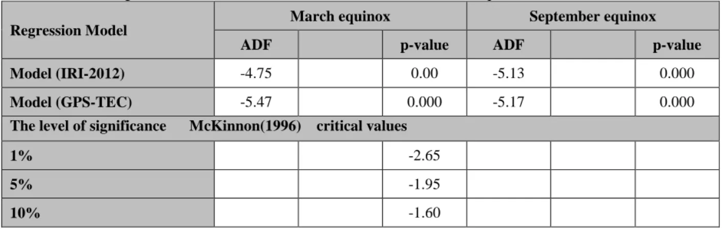
After determining stationarity of dependent and independent variables, co-integration test is applied to the variables to identify whether there is a long-term relationship between the variables or not. The presence of long-term relationship between the variables according to the setup models (eq. (4 and 5)) for the

dependent variables is given at Table 6. To be a long-term relationship between the variables, it is required that the ADF values of the models are greater than McKinnon critical values in absolute value and the p-value is smaller than 0.005. Thus, we can say that there is a long-term relationship between the variables.

Table 6.The co-integration test results for IRI-2012 and GPS-TEC values on equinox months at 24:00 UT.

Regression Model

March equinox September equinox

ADF p-value ADF p-value

Model (IRI-2012) -4.75 0.00 -5.13 0.000

Model (GPS-TEC) -5.47 0.000 -5.17 0.000

The level of significance McKinnon(1996) critical values

1% -2.65

5% -1.95

10% -1.60

After determining the stationarity of variables and detecting there is a long-term relationship between the variables, the following equations are derived by eq. (1) depending on stationarity of the variables:

For IRI-24.00; ε D(F10.7) 2 β ) P (N 1 β )) P (D(V 0 β c 2400 TEC) (IRI D + + + + = − (4) For GPS-TEC-24.00; ε D(F10.7) 2 β ) P (N 1 β )) P (D(V 0 β c 2400 TEC) (GPS D + + + + = − (5)

where c is constant, βsis coefficient of variables and ε is

error term.

The results obtained by the occurred models are shown at Table 7. The results obtained for IRI-2012-TEC dependent variable indicate that the variation of one unit in

V

_p

and F10.7leads to an increase of 2

×

1012 _e/m2 _and

296

×

1012 _e/m2 _{in IRI-2012-TEC values on March}

month, respectively. However, the variation of 1 N/cm3

in

N

_p

causes a decrease of 67

×

1012 _e/m2 _in

IRI-2012-TEC values. Thus, F10.7 cm solar flux has the greatest

effect on IRI-2012-TEC values, whereas

V

_p

has smallest

by independent variables of dependent variable for multiple relationship is rate of 57 %.

For September month, the variation in

V

_p

of 1 km/s and

p

N

of 1 N/cm3 _{results in a decrease of 6}

×

₁₀12 _e/m2 _and

60

×

1012 _e/m2 _{in IRI-2012-TEC values, respectively.}

However, the variation of 1 unit at F10.7 cm solar flux

brings about an increase of 249

×

1012 _e/m2 _in

IRI-2012-TEC values. Hence, whereas F10.7 cm solar flux has the

greatest effect on IRI-2012-TEC values,

V

_p

has smallest

effect on it. The value of Adj. R2 _{is 51% and it indicates}

explicable by independent variables of the part of 57% of changes occurred in dependent variables. The rest of 49% depends on other variables indicating c (constant) coefficient.

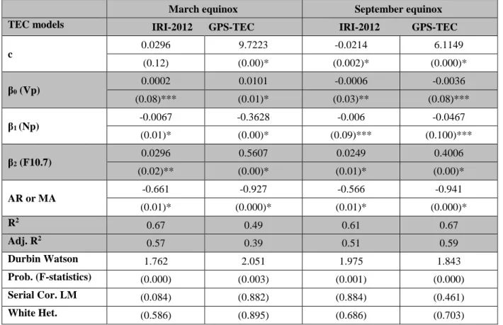
Table 7. Regression analysis results for equinox months at 24:00 UT

March equinox September equinox

TEC models _{IRI-2012 GPS-TEC IRI-2012 GPS-TEC}

c 0.0296 9.7223 -0.0214 6.1149 (0.12) (0.00)* (0.002)* (0.000)* β0 (Vp) 0.0002 0.0101 -0.0006 -0.0036 (0.08)*** (0.01)* (0.03)** (0.08)*** β1 (Np) -0.0067 -0.3628 -0.006 -0.0467 (0.01)* (0.00)* (0.09)*** (0.100)*** β2 (F10.7) 0.0296 0.5607 0.0249 0.4006 (0.02)** (0.00)* (0.01)* (0.00)* AR or MA -0.661 -0.927 -0.566 -0.941 (0.01)* (0.000)* (0.01)* (0.000)* R2 0.67 0.49 0.61 0.67 Adj. R2 0.57 0.39 0.51 0.59 Durbin Watson _{1.762 2.051 1.975 1.843} Prob. (F-statistics) _{(0.000) (0.003) (0.001) (0.000)} Serial Cor. LM _{(0.084) (0.882) (0.884) (0.461)} White Het. _{(0.586) (0.895) (0.686) (0.703)}

*,**,*** represents the significant level at 1%, 5%, and 10%, respectively.

When the results obtained for GPS-TEC dependent variable are investigated, it is observed that the variation

in

V

_p

of 1 km/s and in F10.7 cm solar flux of 1 unit leads

to an increase of 101

×

1012 _e/m2 _{and 5607}

×

₁₀12 _e/m2 _in

GPS-TEC values on March month. However, the

variation of 1 N/cm3 _in

p

N

brings about a decrease of

3628

×

1012 _e/m2 _{in GPS-TEC values. Accordingly,}

F10.7 cm solar flux has the greatest effect on GPS-TEC

values, whereas

V

_p

has smallest effect on it. Adj. R2

value expressed as explainable rate by independent variables of dependent variable for multiple relationship is rate of 39 %. The rest of 61% depends on other variables indicating c (constant).

For September month, it is observed that the relationship between the variables is positive. In that case, an increase

of 1 unit in the

V

_p

and

N

_p

causes an increase of 36

×

1012_{and 467}

×

₁₀12 _e/m2_{. However, the variation of 1 unit}

at F10.7 cm solar flux brings about a decrease of 4006

×

1012 _e/m2 _{in IRI-2012-TEC values. The value of Adj. R}2

is 57% and it indicates explicable by independent variables of the part of 59% of changes occurred in dependent variables. The rest of 41% depends on other variables indicating c (constant) and this rate is explainable by other parameters effecting on GPS-TEC.

4. Conclusions

The following results are obtained by our multiple

regression model set up by Vp,

N

_p

, F10.7 solar flux

parameters and TEC values from mid-latitude station for IRI-2012 and IONLAB models at 12:00 and 24:00 UT on March and September equinox months of 2009 year: • It is observed that the independent variables are

affected over the dependent variables on both March and September month.

• The effecting coefficients of

V

_p

and

N

_p

independent variables are greater at 12:00 UT than 24:00 UT for both IRI-2012 and IONOLAB-TEC models at both months. However, this situation is opposite for F10.7 solar flux values expect for IONOLAB-TEC on September month.

• The order of effecting rates of independent variables

on dependent variables in all cases is as F10.7>

N

_p

>

V

_p

.

• The Adj.R2 _{values which are expressing the}

percentage of effecting of independent variable over the dependent variables are greater at 12:00 UT than 24:00 UT.

• The effect on IONOLAB model of all three parameters is greater than IRI-2012 model for both each months and 12:00 and 24:00 UT.

• While

N

_p

has a negative effect on dependent

variables, F10.7 solar flux has a positive effect on dependent variables at all cases.

References

1. Gorney D.J, Solar cycle effects on the near-earth space environment. Reviews of Geophys, 1990; 28: 315–336.

2. Forbes J.M, Bruinsma S, Lemoine F.G, Solar rotation effects in the thermospheres of Mars and Earth, Science, 2006; 312: 1366–1368. 3. Liu, L, Wan, W, Chen, Y, Le, H, Solar activity effects of the ionosphere: A brief review, Chinese Science Bulletin, 56(12), 2011; 1202-1211.

4. [4] Budden, K.G, The ionosphere and magnetosphere. In the propagation of radio waves; Cambridge Univ. Press: New York, USA, 1988; pp 1-20.

5. Tuna, H, Arikan, O, Arikan, F, Regional model-based computerized ionospheric tomography using GPS measurements: IONOLAB-CIT, Radio Science, 2015, 50(10), 1062-1075.

6. Arikan, F, Shukurov, S, Tuna, H, Arikan, O, Gulyaeva, T.L, Performance of GPS slant total electron content and IRI-Plas-STEC for days with ionospheric disturbance, Geodesy and Geodynamics, 2016, 7(1), 1-10.

7. Chauhan V, Singh, O.P, A morphological study of GPS–TEC data at Agra and their comparison with the IRI model, Advances in Space

Research, 2010, 46, 280–290.

8. da Costa, A.M, Boas, J.W.V, da Fonseca Jr, E.S, GPS total electron content measurements at low latitudes in Brazil for low solar activity,

Geophysica Inter-Nacional, 2004, 43 (1), 129–137.

9. Ezquer, R, Brunini, C, Mosert, M, Meza, A, del, R, Oviedo, V, Kiorcheff, E, Radicella, S, GPS-VTEC measurements and IRI predictions in the South America sector, Advances in Space Research, 2004, 34 (9), 2035–2043.

10. Olwendo, O. J, Baki, P, Mito, C, Doherty, P, Characterization of ionospheric GPS Total Electron Content (GPS–TEC) in low latitude zone over the Kenyan region during a very low solar activity phase,

Journal of Atmospheric and Solar-Terrestrial Physics, 2012, 84, 52-61. 11. Rama Rao, P.V.S, Gopi Krishna, S, Niranjan, K, Prasad, D.S.V.D, Temporal and spatial variation in TEC using simultaneous

measurements from the Indian GPS network of receivers during low solar activity period of 2004–2005, Annales Geophysicae, 2006, 24 (12), 3279–3292.

12. Sezen, U, Arıkan, F, Arikan, O, Ugurlu O. A, Sadeghimorad, "Online, Automatic, Near-Real Time Estimation of GPS-TEC: IONOLAB-TEC", Space Weather, 2013, 11, 1-9.

13. Yizengaw, E, Moldwin, M.B, Galvan, D, Iijima, B.A, Komjathy, A, Mannucci, A. J, Global plasmaspheric TEC and its relative contribution to GPS TEC, Journal of Atmospheric and

Solar-Terrestrial Physics, 2008, 70(11–12), 1541–1548.

14. Liu, L, Wan, W, Zhang, ML, Zhao, B, Case study on total electron content enhancements at low latitudes during low geomagnetic activities before the storms, Annals of Geophysics, 2008, 26, 893–903. 15. Bagiya M.S, Joshi H.P, Iyer K.N, Aggarwal M, Ravindran S, Pathan B.M, TEC variations during low solar activity period (2005– 2007) near the Equatorial Ionospheric Anomaly Crest region in India,

Annals of Geophysics, 2009, 27(3), 1047–1057.

16. Jain A, Tiwari S, Jain S, Gawl A.K, Nighttime enhancements in TEC near the crest of northern equatorial ionization anomaly during low solar activity period, Indian Journal of Physics, 2011, 85(9), 1367–1380.

17. Zou S, Moldwin M.B, Coster A, Lyons L.R, Nicolls M.J, GPS TEC observations of dynamics of the mid latitude trough during substorms.

Geophysical Research Letter, 2011, 38, L14109.

18. Sojka J, David M, Schunk R.W, Heelis R.A, A modeling study of the longitudinal dependence of storm time midlatitude dayside total electron content enhancements, Journal of Geophysical Research, 2012, 117, A02315.

19. Kumar S, Priyadarshi S, Gopi Krishna S, Singh A.K, GPS-TEC variations during low solar activity period (2007–2009) at Indian low latitude stations, Astrophysics and Space Science, 2012, 339(1), 165– 178.

20. Kumar, S, Tan, E. L, Murti, D. S, Impacts of solar activity on performance of the IRI-2012 model predictions from low to mid latitudes, Earth, Planets and Space, 2015, 67(1), 1-17.

21. Bilitza, D, International reference ionosphere 2000, Radio Science, 2001, 36(2), 261–275.

22. Bilitza, D, Reinisch, B.W, International reference ionosphere 2007 improvements and new parameters, Advances in Space Research, 2008, 42(4), 599–609.

23. Anderson, D.N, Mendillo, M, Herniter ,B.A, semi-empirical low latitude ionospheric model, Radio Science, 1987, 22(2), 292–306. 24. Daniell, R.E, Brown L.D, PRISM, A Parameterized Real-Time Ionospheric Specification Model Version 1.5. 1995; Computational Physics Inc, Newton.

25. Nava, B, Coisson, P, Radicella, S.M, A new version of the NeQuick ionosphere electron density model, Journal of Atmospheric

and Solar-Terrestrial Physics, 2008, 70(15), 1856–1862.

26. Scherliess, L, Schunk, R.W, Sojka, J.J, Thompson, D.C, Zhu, L, Utah State University Global Assimilation of Ionospheric Measurements Gauss-Markov Kalman filter model of the ionosphere: Model description and validation, Journal of Geophysical Research, 2006, 111, A11315.

27. Arikan, F, Erol, C.B, Arikan, O, Regularized estimation of vertical total electron content from Global Positioning System data, Journal of

28. Arikan, F, Nayir, H, Sezen, U, Arikan, O, Estimation of single station interfrequency receiver bias using GPS-TEC, Radio Science, 2008, 43(4), RS4004.

29. Bilitza, D, Altadill, D, Zhang, Y, Mertens, C, Truhlik ,V, Richards, P, McKinnell, L-A, Reinisch, B, The International Reference Ionosphere 2012 - a model of international collaboration, Journal of

Space Weather and Space Climate,2014, 4(A07), 1–12.

30. Alcay, S, Yigit, C. O, Seemala, G, Ceylan, A, GPS-Based Ionosphere Modeling: A Brief Review. Fresenius Environmental

Bulletin, 2014, 23, 815-824.

31. Arikan, F, Shukurov, S, Tuna, H, Arikan, O, Gulyaeva, T. L, Performance of GPS slant total electron content and IRI-Plas-STEC for days with ionospheric disturbance, Geodesy and Geodynamics, 2016,

7(1), 1-10.

32. Enders, W, Applied Econometric Times Series; John Wiley and Sons. Inc. New York, USA, 1995.

33. Atıcı, R, Sağır, S, The effect of QBO on foE. Advances in Space Research, 2017, 60, 357-362.

34. Sağır, S., Atıcı, R., Özcan, O., Yüksel, N. The effect of the stratospheric QBO on the neutral density of the D region. Annals of

Geophysics, 2015; 58(3), A0331.

35. Atici, R, Sagir, S, The Effect on Sporadic-E of Quasi-Biennial Oscillation. Journal of Physical Science and Application, 2016, 6(2), 10-17.

36. Kurt, K, Yeşil, A, Sağir, S, Atici, R, The Relationship of Stratospheric QBO with the Difference of Measured and Calculated NmF2. Acta Geophysica, 2016, 64(6), 2781-2793.

37. Zakharenkova, I.E, Cherniak, I.V, Krankowski, A, Shagimuratov, I. I, Vertical TEC representation by IRI 2012 and IRI Plas models for European midlatitudes. Advances in Space Research, 2015, 55(8), 2070-2076.

38. Arunpold, S, Tripathi, N.K, Chowdhary, V.R, Raju, D.K, Comparison of GPS-TEC measurements with IRI-2007 and IRI-2012 modeled TEC at an equatorial latitude station, Bangkok, Thailand,

Journal of Atmospheric and Solar-Terrestrial Physics, 2014, 117,

88-94.

39. Chakraborty, ., Kumar, S, De, B.K, Guha, A, Latitudinal characteristics of GPS derived ionospheric TEC: a comparative study with IRI 2012 model, Annals of Geophysics, 2014, 57, 5.

40. MacKinnon, J.G, Numerical distribution functions for unit root and cointegration tests. Journal of Applied Econometrics, 1996, 11, 601– 618.

41. Özgüç, A, Ataç, T, Pektaş, R, Examination of the solar cycle variation of foF2 for cycles 22 and 23. Journal of Atmospheric and

Solar-Terrestrial Physics, 2008, 70 (2), 268-276.

42. Kutiev, I., Tsagouri, I., Perrone, L., Pancheva, D., Mukhtarov, P., Mikhailov, A, et al., Solar activity impact on the Earth’s upper atmosphere. Journal of Space Weather and Space Climate, 2013 3, A06.