IEEE TRANSACTIONS ON AUTOMATIC CONTROL, VOL. 38, NO. 11, NOVEMBER 1993 1707
IV. CONVERGENCE ANALYSIS OF THE SOLUTION OF THE P R D E
In this section, we investigate the convergence of the solution of the P R D E with a given initial condition to a positive semidef- inite stabilizing or strong solution of the PRDE. This question is of relevant importance to the H, state estimation problem for periodic systems as it ensures that a finite horizon estimator gain will tend to a infinite horizon periodic estimator gain as the time-horizon tends to infinity.
Theorem 4.1: Suppose (C(.), A ( . ) ) is detectable, ( A ( . ) , B(.)) is controllable and that the P R D E (7) has a strong (or stabilizing) solution P,(.) 2 0. Let P ( t ) be the solution of the P R D E with initial condition P(0) 2 0. If P5(0) 2 P(0) then
lim [ P , ( t ) - P ( t ) ] = 0. I + ,
Proof: Let P , ( t ) denote the solution of (7) with P,(0) = 0. From Lemma 3.2, P , ( t ) is periodically nondecreasing and by Lemma 3.1 P,(t) I P,(t> for all t 2 0. Then, P , ( t ) should con- verge to a positive semidefinite periodic solution,
PI(.),
of (7) as t tends to infinity andPI(.>
I P,(.>. Note that by Lemma 3.3, P,(t) and P,(t) are nonsingular for any t . In addition, recalling that from Theorem 3.3 P,(.) is the minimal positive definite periodic solution of the PRDE, we conclude thatF , ( . )
=P,(.).
Now, since 0 I P(0) I P5(0), by Lemma 3.1 it results that for all t 2 0
P , ( t ) I P ( t ) I P,(t>.
Finally, since P , ( t ) converges to P , ( t ) as t tends to infinity, Theorem 4.1 guarantees that subject to the detectability of (C(.), A ( . ) ) and the controllability of ( A ( . ) , E(.)), the finite horizon H, estimator of [11] for the system (Z) converges to the infinite horizon periodic filter of Theorem 3.2 (or Theorem 3.1) as the time-horizon tends t o infinity.
It should be noted that the controllability requirement in Theorem 4.1 can be weakened to stabilizability. This is easily achieved by assuming, without loss of generality, that A ( . ) and B ( .) are in the canonical form (see [2])
hence P ( t > will also converge to P,(t>. v v v
where A , ( . ) is asymptotically stable and the periodic pair ( A , ( . ) , B,(.)) is controllable. Hence, the result follows by decomposing the P R D E conformably with (29) and applying Theorem 4.1 t o the controllable part ( A , ( . ) , B,(.)).
V. CONCLUSION
This note has analyzed the H, state estimation problem for linear periodic systems. Necessary and sufficient conditions for the existence of a periodic state estimator have been derived, which extend existing H, estimation results to the context of linear periodic systems. Asymptotic properties of finite horizon H, estimators for linear periodic systems when the time-horizon tends to infinity have also been investigated.
REFERENCES
[I] D. S. Bernstein and W. M. Haddad, “Steady-state Kalman filtering with an H, error bound,” Syst. Confr. Lett., vol. 12, pp. 9-16, 1989. [2] S. Bittanti and P. Bolzern, “Stabilizability and detectability of
linear periodic systems,” Syst. Contr. Lett., vol. 6, pp. 141-145, 1985.
S. Bittanti and P. Colaneri, “A monotonicity result for the periodic Riccati equation,” in Proc. MTNS’89, Amsterdam, The Nether- lands, June 1989, pp. 83-93.
S. Bittanti, P. Colaneri, and G. Guardabassi, “Analysis of the periodic Lyapunov and Riccati equations via canonical decomposi- tion,” SIAMJ. Contr. Opfimiz., vol. 24, pp. 1138-1149, 1986.
-, “The extended periodic Lyapunov lemma,” Automatica, vol. 21, pp. 603-605, 1985.
S. W. Chan, G. C. Goodwin, and K. S. Sin, “Convergence proper- ties of the Riccati difference equation in optimal filtering of nonstabilizable systems,” IEEE Trans. Aufomat. Confr., vol. AC-29, pp. 110-118, 1984.
C. E. de Souza, “Riccati differential equation in optimal filtering of periodic nonstabilizable systems,” Int. J. Contr., vol. 46, pp. J. C. Doyle, K. Glover, P. P. Khargonekar, and B. A. Francis, “State-space solutions to standard H , and H, control problems,”
IEEE Trans. Automat., Contr., vol. 34, pp. 831-847, 1989.
G. A. Hewer, “Periodicity, detectability and the matrix Riccati equation,” SIAM J. Contr. Opfimiz., vol. 13, pp. 1235-1255, 1975. H. Kano and T. Nishimura, “Periodic solutions of matrix Riccati equation with detectability and stabilizability,” Znf. J. Confr., vol. 29, pp. 471-487, 1979.
K. M. Nagpal and P. P. Khargonekar, “Filtering and smoothing in an H, setting,” IEEE Trans. Automat. Contr., vol. 36, pp. 152-166, 1991.
U. Shaked, “H, minimum error state estimation of linear station- ary processes,” IEEE Trans. Automat. Contr., vol. 35, pp. 554-558, 1990.
M. A. Shyman, “Inertia theorems for the periodic Lyapunov equa- tion and periodic Riccati equation,” Syst. Contr. Lett., vol. 4, pp. I. Yaesh and U. Shaked, “Game theory approach to optimal linear estimation in the minimum H,-norm sense,” in Proc. 28th IEEE
Con6 Decision Contr., Tampa, FL, Dec. 1989, pp, 415-420.
1235-1250, 1987.
27-32, 1984.
Adaptive Robust Sampled-Data Control of a Class of Systems Under Structured Perturbations
Runyi Yu, Ogan Ocali, and M. Erol Sezer
Abstract-Robust adaptive sampled-data control of a class of linear systems under structured perturbations is considered. The controller is a time-varying state-feedback law having a fixed structure, containing an adjustable parameter, and operating on sampled values. The sampling period and the controller parameter are adjusted with simple adaptation rules. The resulting closed-loop system is shown to be stable for a class of unknown perturbations. The same result is also shown to be applica- ble to decentralized control of interconnected system.
I. INTRODUCTION
Robust control problem is concerned with the design of con- trollers which guarantee certain desired properties for all sys- tems belonging to a specified class. Although numerous results have been obtained for both continuous- and discrete-time ro- bust control (see, for example, [ 1]-[5] and the references therein), most of the research on robust control of sampled-data systems has been concentrated o n analysis of robustness properties (e.g., [6], [7]). This is mainly due to the fact that the sampling process changes the structure of systems, which makes the problem difficult to deal with. For example, the sampling process may
Manuscript received January 3, 1992; revised October 2, 1992. The authors are with the Department of Electrical and Electronics Engineering, Bilkent University, 06533 Bilkent, Ankara, Turkey.
IEEE Log Number 9208717. 0018-9286/93$03.00 0 1993 IEEE
1708 IEEE TRANSACTIONS ON AUTOMATIC CONTROL, VOL. 38. NO. 11, NOVEMBER 1993 give rise to unstable zeros in the resulting discrete-time system
even when the continuous-time system is of minimal phase [8]. Recently, Ocali, and Sezer [9] considered the robust sampled- data control problem for a class of systems under structured perturbations. Under the assumptions that the perturbations are bounded and the bounds are known, they presented a control scheme which included the determination of the sampling period and the controller parameters in terms of the bounds of the perturbations. One of the objectives of our paper is to propose a mechanism to adjust these parameters adaptively, eliminating a need for a priori information o n the perturbation bounds. A second objective is to simplify the control structure. Although theoretically, the feedback law presented in [9] can also be used in adaptive control, it is difficult to implement this control in practice, since it involves the computation of an exponential function of a matrix at every sampling period. To avoid this difficulty, we provide an alternative structure for the feedback law with adjustable parameters including the sampling period. We show that under certain assumptions concerning the struc- ture of perturbations, the resulting closed-loop adaptive sam- pled-data control system is stable in the sense that the state of the system goes to zero exponentially and the adaptation param- eters consisting of sampling periods and feedback gains converge to constant numbers which depend on the initial conditions of the system. We also consider the same problem for intercon- nected systems in the framework of decentralized control and central adaptation.
11. PROBLEM STATEMENT AND PRELIMINARIES We consider a single-input system Y described as
9: x ( t ) = [ A
+
H ( t ) ] x ( t )+
b u ( t ) (2.1) where x ( t > ~ 9is the state and ~ ( t ) 2 ~ is the input of 9; A and b are constant matrices of appropriate dimensions; and H ( t ) represents additive perturbations.We assume that the pair ( A , b ) is controllable, and is in the canonical form
where a,, 1 = 1,2;.., n , are constant but unknown parameters. of the form
T o the system 9, we apply a sampled-data feedback control
~ ( t ) = k r ( t - t,, y,)x(t,), t , 5 t
<
t,+ 1 (2.3) where t , denote the sampling instants, y, is a parameter which is constant over each sampling interval [t,, t,+ ,), but may change from one interval to another, and k ( t , y ) is a time-vary- ing feedback gain vector, which is a bounded function of f for every fixed y .We further assume that H ( t ) has a lower-triangular structure
I
:
:
I
where h,,, p , q = 1,2;.., n , are unknown bounded functions with bounded derivatives of all orders up t o n - 1. There are two reasons for restricting H ( t ) to have this structure. The first
is that n o controller could provide robust stability for all pertur- bations of a more general structure. A simple example is a constant H which nullifies the 1's in A of (2.2). The second reason is that Y is known [lo] to be stabilizable by a high-gain continuous-time state feedback control against all bounded per- turbations of the form (2.41, provided their bounds are known a priori. In fact, our first objective is to reproduce the same result with the sampled-data controller in (2.3), and the second objec- tive is to eliminate the need for the information about the bounds of the perturbations.
With the control in (2.3) applied to 9', the resulting closed-loop system becomes
9:
X ( f ) = [ A+
H ( t ) l x ( t )+
bk'(t - t,, y,)x(t,), t, 5 t<
t,+, (2.5) the solution of which is given by [ 111x ( t ) =
6(t,
t , , y,>x(t,>, t , 5 t<
t,,, I (2.6) where6 ( ( ,
f,, y,,,) = W t , t m )+
1'
W t , r)bkT(7-
t,, y,) d~ (2.7) with @ ( t , t,) being the state transition matrix of 9'. Evaluating (2.6) at t = t,+ ,, we obtain&:
x(t,,,) = 6 ( t m T , , t , . y m ) x ( t , ) (2.8)'"7
which defines a discrete-time system.
Suppose that the sampling periods, defined as
Tm = t m + l - t m (2.9) are bounded from above, and that Iim,,+=t,,, = E. Then, for any t
>
t,,, there exists an m such that t,,, I t I t m + , . Since @ ( t , 7 )and k ( t , y,) are bounded fpr all t and T with t , I T I t I t,,
,,
it follows from (2.6) that 9 in (2.5) is stable in continuous sense if and only if 9 in (2.8) is stable in discrete sense. Our immediate purpose is to choose a suitable structyre for the gain k T ( t , y ) in (2.3) which guarantees stability of 9 under certain conditions on y, and T,. For this purpose, we refer to 191, who used a time-varying feedback gain of the formk T ( t , y ) = k T ( y ) e x p { [ A , )
+
bkT(y)lt} (2.10) where A , has the same structure as A in (2.2) with the last row elements replaced by zeros, and k r ( y ) is a constant gain which places the eigenvalues of A ,+
bk'(y) at - p l y with p l>
0, 1 = 1,2,....
n , being arbitrary distinct numbers. It has been shown in [9] that with the sampling periods T, and the parameters y,,, kept constant as T, = T and 7, = y , there exist T'">
0 and y *>
0, which depend on the bounds o n the perturbations, such that the sampled-daia control in (2.3) with the gain as in (2.10) results in a stable 9 for all T<
T * and y>
y * . (Note that a simple discretization of a high-gain continuous-time controller would require smaller T for larger y . Thus, the result of 191 is not a straightforward translation of an analog controller to digital domain.) The motivation behind the present work is to relax the requirement that these bounds be known by adjusting the sampling period T, and the parameter 7, adaptively.A closer examination of the gain in (2.10) reveals that its components behave like lst, 2nd, etc., order impulses. Motivated by this observation, we choose the structure of the gain vector k T ( t . y ) in (2.3) as
IEEE TRANSACTIONS ON AUTOMATIC CONTROL, VOL. 38, NO. 1 1 , NOVEMBER 1993
with components
(2.12) where p,[
>
0 are arbitrary distinct numbers, and the coefficientsair are obtained by solving the equations
(2.13) It is easy to check that k , ( t , y ) behaves like an I-th order impulse for large y . That is, limy /? f(t)k,(t, 7) dt = ( - l)'f('- l ) (0) for any function
f
which is infinitely differen-tiable at t = 0.
We next ipvestigate the behavior of the discrete state transi- tion matrix @ ( t m + l , t,, y,) in (2.8) for fixed T, and y,. For this purpose, we define as in [9] the vectors
z , ( t ) = b ,
z I + , ( t ) = [ A
+
H ( t ) ] z , ( t ) - , i / ( t ) , I = 1,2;.., n , (2.14)and form the matrix
Z ( t ) = [ z , ( t ) z , - 1 ( t ) . . . z , ( t ) l . (2.15) From (2.71, we write & t , t , , y,) = @ ( t , t,)W(t,>
+
* ( t , t,,, 7,) (2.16) where and W ( t ) =I -
Z ( t ) (2.17) ~ t , t , , y ) = ~ ( t , t,)z(t,)+
/ I ~ ( t , T ) b k T ( T - t,, y ) d7 f m (2.18) and state the following.bounded, then
Lemma 2.1: If H ( t ) and its derivatives up to order n - 1 are
lim ?(t,t,, y ) = 0 (2.19) Y+% for all t
>
t,. Pro06 Let V r ( t , t , , y ) = [ 4 J n ( t , t , , Y ) ' . . 4 J l ( t , t , > Y ) I . (2.20) We claim that4,(t,
t,, y ) = / I ( - l ) S y ' - ~ r - ~ I C y l , e - " ' r Y ( ' - ' n l ) z S ( t ) ~ =r = l l I + ( - 1)' C Y l . 4 ' ~ ( ~ , T ) ~ ~ + l ( T ) ~ ~ ~ r Y ( T ~ ' ' r " d ~ . (2.21) r = 1The claim can easily be proved by showing using (2.12)-(2.14) and (2.18) that both sides of (2.21) satisfy the same differential equation
[ ( t ) [ A
+
H ( t ) ] [ ( t >+
b k / ( t - t,, 7)[ ( t , ) = z,(t,). (2.22)
~
1709
The proof then follows from the boundedness of z,(t), 1 =
1,2;.., n
+
1, which is implied by the boundedness of H ( t ) and its derivatives.From (2.16) and Lemma 2.1 we observe that withAk(t, y ) chosen as in (2.11)-(2.13), and y, sufficiently large, @(t,+l,
t,, Y,~) in (2.8) behaves essentially like @(t,,+ I, t,)W(t,), which is independent of y,. This observation, together with the struc- ture of W(tn,) implied by the structure of
q(t),
allows us to reach the following result o n the stability of 9.Theorem 2.1: Let k T ( t , y ) be chosenAas in (2.11)-(2.13). Then
there exist T *
>
0, y *>
0 such that 9 in (2.8) is exponentially stable provided that y, I y * , 0<
T,,, I T * , m E Z+.Proof: We first observe that boundedness of H ( t ) and its
derivatives, (2.14), (2.17), (2.18) and Lemma 2.1 imply that M , = sup IlW(t)Il
1E.W
€(I-)
= sup sup l1@(tm+1,tm) -1110 < T,,, s T t,,, €9
6 ( T , y ) = sup sup sup l l ~ ( f m + l , f , , y , ) ~ ~ (2.23)
y"! 2 y 0 T", c T I", €9 all exist, and that
lim E ( T ) = 0
T + 0
lim 6 ( T , y ) = 0, for all T
>
0 Y + =From (2.8) we have
Taking the norm of both sides of (2.251, expanding the product using (2.16), and using (2.23) and (2.241, we obtain
( n - 1
provided T,, I T and y, 2 y , m E X + , where we use the nota- tion W,+/ = W(t,+/), @,+/ = @ ( t , + / + l , l,+/), for conve- nience. Now using the identity
(2.27) and (2.23), the product term in (2.26) can further be bounded as
@ r n + / W l + /
= W,i/+
[@,+/ - IIW,+/provided T, I T .
lower triangular matrix with zero diagonal elements, so that As can easily be seen from (2.4), (2.14), and (2.171, W ( t ) is a
n - 1
I =
n
0WWl+/ = 0 (2.29)
(2.24), (2.28), and (2.29) imply that for any p 1
>
0, there exists a T*>
0 such that1 1 - 1
n
Il@"+/Wm+/ll 5 PI (2.30) / = o1710 IEEE TRANSACTIONS ON AUTOMATIC CONTROL, VOL. 38, NO. 11, NOVEMBER 1993 provided T, I T * , m E % + . With T* futed to satisfy (2.30),
(2.24), and (2.26) imply that for any p 2
>
0, there exists a y *>
0 such that provided T, I T * , y, 2 y * , m E X + . Let p = pi+
p 2<
1. Withr
r - 1 1 we have from (2.31) Ilx(t,>ll I M ( p"">mllx(to)ll (2.33) and the proof follows.We observe from the proof of Theorem 2.1 that for given p1 and p , , T * and y* depend on the bounds of H ( t ) and its derivatives, which are unknown. This necessitates the use of an adaptation mechanism to adjust T, and y, based on measure- ments of x(t,). In the next section, we investigate this problem.
111. ADAPTIVE SAMPLED-DATA CONTROL
We choose the adaptation rules for the sampling period T, = t m + l - t,, and the parameter y, in k ( t - t,, y,) of (2.3) as
T i l i = T;l
+
(T711x(tm)llym+l = y,
+
qllx(t,)ll (3.1)where a,,
q ,
To, y o>
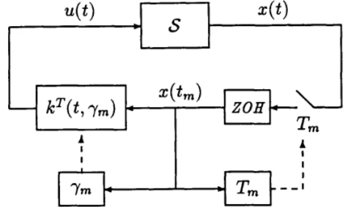
0 a r e arbitrary. Thus, the closed-loop adaptive control system .Y in (2.5) has the configuration shown in Fig. 1.The system
4
in (2.8) associated with9,
and the adaptatipn rules in (3.1) define a discrete-time adaptive control system gA, whose solutions starting from the initial condition x A ( t o ) =(xo, To, yo), we denote by x A ( t m ; x o , 7-0, y o ) = [x(t,), T,, Y,,,]. The following theorem states our main result.
Theorem 3.1: Under the feedback control in (2.3) with k ( t , y ) chosen as in (2.11)-(2.13), and T, and y, adjusted according to (3.11, we have lim T,,, = T,
>
0, (3.2) nl + 5 lim y, = y .>
0. (3.3) ni --t = lim x(t,) = 0 m 4 = (3.4) so that x,(t,; xo, To, yo) is bounded for all To>
0, y o>
0 and P Y O O ~ Let T* and y * be as in the statement of Theorem x(t,) = xg.2.1. Three cases are possible. Case I) T,
>
T* for all m E Z + .In this case, since {T,) is nonincreasing, T, 2 T * exists, prov- ing (3.2). Then, (3.4) follows directly from (3.1). (3.1) also implies that m - 1 T i l = T;i
+
(T7 IlX(t/)lI (3.5) 1 = 0 so that y, = yo+
((Ti//cTT)(T;l - T i i ) (3.6)and (3.3) follows by taking the limit. Case
II)
y,<
y * for all m EX+.In this case, the proof follows exactly the same lines as the proof of Case I) with the roles of y, and T; interchanged.
Fig. 1. Structure of the adaptive sampled-data control system.
Case I I I ) T, I T* for some m T E Z + , and y, 2 y * for some
my E X + .
Let m* = max{m7, my). Then, since {T,) is nonincreasing, and {y,} is nondecreasing, we have T, I T* and y, 2 y * for all m 2 m*. Theorem 2.1 implies that
ilx(t,)ll
I ~ p , " - ~ * l l x ( t , * ) l l , m 2 m* (3.7) where p o = pi"', and p<
1 is as in the proof of Theorem 2.1 (3.7) directly implies (3.4). Also,m - 1
/ = m *
and similarly
(3.8)
(3.9) so that both T,
>
0 and yr>
0 exist. This completes the proof. Example 3.1: T o illustrate the result of Theorem 3.1 we con- sider a second order system withA = [ : :
:I
to which we apply a sampled-data control of the form in (2.3). Choosing p i = 1, p, = 2 arbitrarily, and solving (2.13) for q r ,
we construct
k T ( t , y ) = [ - y e - " ' 2y'e-Y' - 4y2e-2''']. (3.10) The solution of the resulting closed-loop system is obtained by numerical integration using Euler method [12] with a time-step of h = 0.01. The elements of the perturbation matrix are gener- ated randomly once every ten integration steps as
h,, = O.OS[rand (1) - 0.71
h,, = 0.40[rand(l) - 0.51 h,, = -0.30[rand(1) - 0.31
where rand( 1) produces a random number uniformly distributed over
[o,
11.The parameters T, and y,,, are updated using (3.1) with uT = uy, = 1. The simulation results corresponding to arbitrarily chosen initial conditions xo = [OS4 - 0.2OlT, To = 0.3 and y o =
~~
IEEE TRANSACTIONS ON AUTOMATIC CONTROL, VOL. 38, NO. 11, NOVEMBER 1993 1711
-0.2
I
I 0 0.5 1 1.5 2 2.5 3 3.5 4 (a) 5I
2 0 0.5 1 1.5 2 2.5 3 3.5 4 (3) 0.6 II
the input at the sampling instants can be clearly seen. It is also observed that the feedback gain converged to an almost periodic steady-state corresponding to T, = 0.15 and y% = 6 in about 20 iterations. Finally, it should be noted that although the bounds of the perturbations are known in this particular example, this information is not used in the design of the control law.
IV. DECENTRALIZED ADAPTIVE SAMPLED-DATA CONTROL The result of the previous section finds a natural application in decentralized control of interconnected systems, where the interconnections among the subsystems are treated as perturba- tions on locally controlled decoupled subsystems.
Consider such an interconnected system consisting of N sin-
-44:
i , ( t ) = A , x , ( t )+
b , u , ( t )+
1 4H,,(t)x,(t), i E N (4.1) where N = {1,2;.., N } ; x , ( t ) ~ 5 % ’ ~ ‘ and u , ( t ) ~ 5 % ’ are the state and the input ofz;
A , and b, are constant matrices having the structure in (2.2); and H,,(t) represent interconnections among the subsystems.Imitating the controller structure in the previous section, we apply to
gle-input subsystems described as
decentralized sampled-data feedback of the form u , ( t ) = k T ( t - t,, y,)~,(t,),t, I t
<
t m + l , i (4.2)1712 IEEE TRANSACTIONS ON AUTOMATIC CONTROL, VOL. 38, NO. 11, NOVEMBER 1993
where each gain vector k , ( t , y ) has the structure in (2.11)-(2.13), except that another index i is appended to k,(t, y ) , air, ,ur and n .
Defining x‘ = [ x F x F
...
xi]’, A’ = d ’ IagIA,, A2;.., A,,,}, B‘ and K’(t, y ) similarly, and H’(t) = [ Hf,(t)lN,,,,
the resultingclosed-loop sampled-data system can be described compactly as
4’:
x’ ( t) = [A’+
H’(t)]x’(t)+
B’K’(t - t,, y,)x’(t,), t , I t<
t,+ 1. (4.3)As in the previous section, we associate with
3’
a discrete-time system& I : x J ( t , + , ) = W t m + , , t m , y , ) x I ( t , ) (4.4) whose stability is equivalent to that of
4’,
where& < t , t,, ym) = @ I ( t , t,)
+
[‘
@.‘(t, T ) B I K ’ ( T - t,, y,) d7 (4.5) with @‘(t, t,) being the state transition matrix associated with A’+
H I ( [ ) .We next establish a counterpart of Lemma 2.1. For this purpose, we define the vectors
z { ( t ) = b,’
z/,,(t) = [ A ’
+
H’(t)]z/(t) - i ; ( t ) ,I
= 1,2;..,n,, j s.4’ (4.6) where 6f = [0...
6:...
01’ is the j-th column of B‘, and con- struct the matricesj E.N (4.7) z;(t) =
[
z ~ , ( t > zi,- , ( t > ... z i ( t ) ] , and Z‘(t) = [ Z 1 ( t ) Z J t ) ... Z,(t)I. (4.8) (4.9) (4.10) Then, with we have W‘(t) = I - Z ’ ( t )6‘(t,
t,, y ) = @ I ( [ , t,>W’(t,>+
“’(t, t,, y ) where “’(t, t,, y ) = @ I ( [ , t,)Z’(t,)+
[‘
@‘(t, T ) B I K ’ ( T - t,, y ) d 7 . (4.11) With these definitions, the proof of the following counterpart of Lemma 2.1 is automatic.Lemma 4.1: The result of Lemma 2.1 remains valid if H ( t ) and “ ( t , t,, y ) are replaced with H I ( [ ) and * ’ ( t L t m , y ) .
T o reproduce the result of Theorem 2.1 for 9‘ of (4.4) we need to restrict the structure of the interconnection matrix. For this, we define the structure index of a matrix D = (d,,) as
m
where m, is a sufficiently large integer. Thus, m ( D ) indicates the position of a diagonal line parallel to the main diagonal, which borders all nonzero elements of D. We assume that for
any index set Z C M , the structure indices of H,,(t) satisfy
. [ m ( H , , ) - 11
<
0. (4.13)[ , I t 9
The reason for assuming this structure for H,,(t) is that they characterize a relatively large class of interconnections which allow for stabilization with continuous-time decentralized state feedback [lo]. Note that for Y = {i}, (4.13) requires that m(H,,)
<
1, that is, H , , ( t ) have the structure in (2.4). We state the following.Lemma 4.2: Let kT(t, y ) , i EM, be chosen as in $2.11)-(2.13). Then there exist T *
>
0 and y *>
0 such that 8‘in (4.4) is exponentially stable provided that y, 2 y * and 0<
T, I T* for all m E Z + .Pro05 The proof follows exactly the same lines as the proof
of Theorem 2.1 with n replaced by n ,
+
n 2+
...
n N . The criti- cal step is to show that (2.29) holds for W,‘ = W’(t,>. The proofof this fact, which has been presented in [9], is technically quite detailed, and therefore, will not be repeated here. T o give an idea about the proof, we only mention that the structural condi- tion in (4.13) implies
(4.14)
for any index set Y c M , where
W,’
= (W/!l,),,N. It is then quite straightforward to show using (4.14) that(4.15) from which the proof follows.
for T, and ynl
We finally employ the following centralized adaptation rules
T i : , = T i ’
+
a , T l l x l ~ t m ~ m , ~ l l1 4
’ y ~ n + I = ym
+
C
~ z y ~ ~ x i ( t m - m I ) ~ ~ (4.16)I EM
where To, yo, a,‘, a , Y
>
0, i E.N; are arbitrary, and the terms corresponding to m - m,<
0 are absent in the summations in (4.16). We note that the delays m,>
0 are introduced in order to provide sufficient time for the centralized adaptation mecha- nism to gather and process information about the subsystem states. Denoting the solutions of the adaptive control system consisting of (4.4) and (4.16) starting from the initial condition (x& To, y o ) by xi(t,; x i , To, y o ) = [x’(t,), T,, y,]‘, we state the following theorem, whose proof follows exactly the same lines as the proof of Theorem 3.1.Theorem 4.1: The result of Theorem 3.1 remains valid if k ( t , y ) and xA(tm; x”, To, y o ) are replaced by K‘(t,
r)
and x i ( t , ; x i , To, Yo).REFERENCES
[l] G. Leitmann, “Guaranteed asymptotic stability for some linear systems with bounded uncertainties,” J. Dynam. Syst. Measurement, Contr., vol. 101, p. 212, 1979.
[2] B. R. Barmish, “Necessary and sufficient conditions for quardratic stabilizability of an uncertain linear system,” J. Optimiz. Theory [3] S. P. Bhattacharyya, Robust Stabilization Against Structured Per- turbations, Lecture Notes in Control and Information Science, vol. 99. New York: Springer-Verlag, 1987.
M. E. Magdna and S. Zak, “Robust state feedback stabilization of
discrete-time uncertain dynamical systems,” IEEE Trans. Automat.
Contr., vol. AC-33, pp. 887-891, 1988.
[5] W.-C. Yang and M. Tomizuka, “Discrete time robust control via state feedback for single input systems,” IEEE Trans. Automat. Contr., vol. 35, pp. 590-598, 1990.
[6] D. S. Bernstein and C. V. Hollot, “Robust stability for sampled-data control systems,” Syst. Contr. Lett., vol. 13, pp. 211-226, 1989. Appl., vol. 46, pp. 399-408, 1985.
IEEE TRANSACTIONS ON AUTOMATIC CONTROL, VOL. 38, NO. 11, NOVEMBER 1993 1713
[7] T. Chen and B. A. Francis, “H,-optimal sampled-data control,” IEEE Trans. Automat. Contr., vol. AC-36, pp. 387-397, 1991. [8] K. J. Astrom, P. Hagander, and J. Sternby, “Zeros of sampled-sys-
tems,” Automafica, vol. 20, pp. 31-38, 1984.
[9] 0. Ocali and M. E. Sezer, “Robust sampled-data control,” IEEE Trans. Automat. Con?., to appear.
[lo]
M. Ikeda and D. D. Siljak, “On decentrally stabilizable large-scale systems,” Automafica, vol. 16, pp. 331-334, 1980.[ll] C.-T. Chen, Linear System Theory and Design. Tokyo: Holt- Saunders, 1984.
[I21 D. Zwillinger, Handbook of DifSerential Equations. New Y o r k Academic Press, 1989.
Low-Order Stabilizing Controllers
D.-W. Gu, B. W. Choi, and 1. Postlethwaite
Abstract-A method for designing low-order stabilizing controllers is described. It is shown that for some plants the order of stabilizing controllers may be less than or equal to I(respectively m ) , where /(respectively m ) is the number of plant outputs(respectively inputs). An
explicit characterization of a set of low-order stabilizing controllers is given and numerical examples are provided to illustrate the results of the note.
I. INTRODUCTION
As the complexity of controllers increases, to meet higher performance specifications using modern methods of design, the order, i.e., the McMillan degree of a controller, becomes a research topic of great practical significance.
For ease of implementation, certification, commissioning, and maintenance, low-order controllers are normally preferred to high-order ones, provided there is no serious deterioration in performance. Various model-reduction methods have been introduced [3], [IO] to reduce the order of a designed controller, but after reduction it is necessary to reanalyze the design to check that any degradation in performance is not too significant. An alternative approach would be to design a lower order controller directly to meet the design objectives.
In this note, we focus on the problem of how to characterize a set of low-order stabilizing controllers.
The problem has already received much attention [l], [6]-[8]. For example, in [l], [7] a lower bound on the order of a (dynamic) stabilizing controller is derived for arbitrary pole placement. Despite such attention, the low-order stabilization problem is largely an open problem and all the existing results provide only suficient conditions for the existence of stabilizing controllers of a certain order. We present in this note a suffi- cient and constructive approach to this open problem. Specifi- cally, we use the celebrated “Youla parameterization” of all stabilizing feedback controllers for a given plant, to present an algorithm in the state-space domain for characterizing the set of (internally) stabilizing controllers of “lowest” possible order; here lowest is with respect to the algorithm used. We also show
Manuscript received May 29, 1991; revised August 5, 1992. This work was supported in part by the U.K. Science and Engineering Research Council.
how to construct a set of stabilizing controllers of given fixed order if a certain condition holds.
The note is structured as follows. In Section 11, the problem of designing low-order stabilizing controllers is reduced to the problem of solving two simultaneous equations, which consist of a Sylvester equation and a linear matrix equation. In Section 111 the special case of stabilizing controllers of order ( n - l ) is considered, and in Section IV the set of stabilizing controllers of smallest possible order using the particular approach of the note is considered. A n explicit characterization for the set of low-order stabilizing controllers is derived in Section V. Some numerical examples are provided to illustrate the results of this note in Section VI and conclusions are given in Section VII.
11. STABILIZING CONTROLLERS
Consider the feedback configuration of Fig. 1, where G(s> is a given plant, and K ( s ) is a controller to be designed for internal stabilization.
Without loss of generality, we assume G(s) is minimal and strictly proper and let G(s) have the state-space realization
where the dimensions of the matrices ( A , B , C ) are n X n , n X m, and I X n , respectively. And C is assumed to be of full column rank.
Also let G(s) have a doubly coprime factorization
G(s) = NM-1 =
G-lI?
(2)and let
X,
Y ,k,
and satisfy the Bezout identity, i.e., ( 3 ) where the matrices ( N , M,I?,
M ,
X,
Y ,k,
9 )
all belong to (the set of all real rational matrices whose elements are stable and proper). The matrices ( N , M ,X,
Y ) can each be expressed in state-space form as follows, by choosing real matrices F and H such that A+
BF and A+
HC are stable [ll]:Y ( s ) :=
[qq-+.
(4)
(5) (6)
( 7 ) Then it is well known [2], [14] that the set of all stabilizing
K ( s ) = - ( Y - M Q ) ( X - N e ) - ’ ,
Suppose that Q(s) has the state-space realization controllers for the given plant G(s) can be parameterized by
for Q ( s )
E H .
(8)I (9)
The authors are with the Control Systems Research, Department of IEEE Log Number 9212880.
Engineering, Leicester University, Leicester LE1 7RH, U.K. with