Electricity consumption and economic growth in Turkey: an MF-var approach

(1)

ELECTRICITY CONSUMPTION AND ECONOMIC GROWTH IN TURKEY: AN MF-VAR APPROACH

A Master’s Thesis

by

D LARA BERKSUN

Department of Economics hsan Do ramacı Bilkent University

Ankara August

(2)

(3)

(4)

The Graduate School of Economics and Social Sciences of

hsan Do ramacı Bilkent University

by

D LARA BERKSUN

In Partial Fulfilment of the Requirements for the Degree of MASTER OF ARTS IN ECONOMICS

THE DEPARTMENT OF ECONOMICS HSAN DO RAMACI B LKENT UNIVERSITY

ANKARA August

(5)

(6)

ABSTRACT

Berksun, Dilara

M.A., Department of Economics Supervisor: Prof. Dr. Hakan Berument

August

This thesis investigates the relationship between monthly electricity consump-tion, quarterly GDP and quarterly components of GDP using a Mixed Fre-quency VAR model for Turkey. The empirical evidence reveals that an increase in electricity consumption increases GDP. However, an increase in electricity consumption increases Private Consumption, Investment, Imports expendi-tures, Construction, Industrial, Manufacturing and Service Sector outputs more than it increases GDP. In addition to this, the empirical evidence reveals that an increase in electricity consumption increases Agricultural sector output less than it increases GDP.

Keywords: Economic Development, Electricity Consumption and Mixed Fre-quency Vector Autoregression Model.

(7)

ÖZET

TÜRK YE’DE ELEKTR K TÜKET M VE KT SAD BÜYÜME

Berksun, Dilara

Yüksek Lisans, ktisat Bölümü Tez Danı manı: Prof. Dr. Hakan Berument

August

Bu çalı mada Türkiye’deki aylık elektrik tüketimi ile çeyreklik Gayri Safi Yur-tiçi Hasıla (GSY H) ve GSY H’nın alt bile enleri arasındaki ili ki Karma Fre-kanslı Vektör Otoregresyon model kullanılarak incelenmi tir. Ampirik sonuçlar elektrik tüketiminin GSY H’yı artırdı ını gösterirken elektrik tüketimindeki ar-tı özel tüketimi, yaar-tırımı, ithalaar-tı ve aynı zamanda in aat, endüstri, imalat, servis sektörlerinin üretimini GSY H’dan daha fazla artırdı ını göstermektedir. Buna ek olarak sonuçlar bize elektrik tüketimindeki artı ın tarım sanayisindeki üretimi GSY H’yı dü ürdü ünden daha fazla dü ürdü ünü göstermektedir.

Anahtar Kelimeler: Elektrik Tüketimi, ktisadi Büyüme ve Karma Frekans Vektör Otoregresyon Model.

(8)

ACKNOWLEDGMENTS

I would first like to thank my thesis advisor Professor Hakan Berument for his continuous support and for always believing in me. I am honored for being able to work with a professor with not just extensive knowledge but also with a big heart. I could not have imagined having a better advisor and mentor. Besides my advisor, I would also like to thank the rest of my thesis committee: Prof. Dr. Erinç Yeldan and Prof. Nükhet Do an for their valuable comments and their support.

I would also like to thank Gül, Gökberk, Arda, Bengi, Humay, Ezgi, Ye im for being the best of friends. Thank you for bringing so much joy, love, support and happiness into my life.

I would like to give special thanks to my parents, Adalet and O uz, for always being by my side and always believing in me. They are the best parents that anyone could ever ask for. I am grateful for the love they have given me all my life. This accomplishment would not have been possible without them. I would also like to thank them for giving me the best gift of my life, Hercules, my cat. He was the most adorable boy.

(9)

LIST OF FIGURES

. Impulse Response Functions based on the VAR( ) model of

quarterly Electricity Consumption (EC) and quarterly GDP . . . . Impulse Response Functions based on the MF-VAR( ) model of

monthly Electricity Consumptions (EC1, EC2, EC3) and quar-terly GDP . . . . . Impulse Response Functions based on the MF-VAR( ) model of

monthly Electricity Consumptions (EC1, EC2, EC3) and quar-terly Private Consumption (P C) . . . . . Impulse Response Functions based on the MF-VAR( ) model of

monthly Electricity Consumptions (EC1, EC2, EC3) and quar-terly Government Spending (GOV ) . . . . . Impulse Response Functions based on the MF-VAR( ) model of

monthly Electricity Consumptions (EC1, EC2, EC3) and quar-terly Investment (INV ) . . . . . Impulse Response Functions based on the MF-VAR( ) model of

monthly Electricity Consumptions (EC1, EC2, EC3) and quar-terly Exports (EX) . . . . . Impulse Response Functions based on the MF-VAR( ) model of

monthly Electricity Consumptions (EC1, EC2, EC3) and quar-terly Imports (IM) . . . . . Impulse Response Functions based on the MF-VAR( ) model of

monthly Electricity Consumptions (EC1, EC2, EC3) and quar-terly Construction Sector output (CONS) . . . . . Impulse Response Functions based on the MF-VAR( ) model of

monthly Electricity Consumptions (EC1, EC2, EC3) and quar-terly Manufacturing Sector output (MAN) . . . .

(11)

. Impulse Response Functions based on the MF-VAR( ) model of monthly Electricity Consumptions (EC1, EC2, EC3) and quar-terly Industrial Sector output (IND) . . . . . Impulse Response Functions based on the MF-VAR( ) model of

monthly Electricity Consumptions (EC1, EC2, EC3) and quar-terly Service Sector output (SERV ) . . . . . Impulse Response Functions based on the MF-VAR( ) model of

monthly Electricity Consumptions (EC1, EC2, EC3) and quar-terly Agricultural Sector output (AG) . . . .

(12)

CHAPTER

INTRODUCTION & LITERATURE REVIEW

There has been a vast amount of literature on the relationship between elec-tricity consumption and GDP. However, in terms of the direction of this causal relationship, the studies vary. While some authors find a unidirectional causal-ity running from one of the variables to the other, others detect a bidirectional causality or no causality at all. The literature has uncovered four possible re-lationships between electricity consumption and economic growth, which has been synthesized into four testable hypothesizes each requiring a different pol-icy implication for energy investment and macroeconomic polpol-icy design (Aper-gis & Payne, : Payne, a). First, the growth hypothesis corresponds to the positive unidirectional causality running from electricity consumption to economic growth. This hypothesis is based on the idea that energy is a fac-tor of production (Csereklyei & Humer, ). Hence, it implies that an in-crease in electricity consumption will cause an inin-crease GDP. Therefore, under the growth hypothesis, implementing policies that reduce electricity consump-tion will hinder economic growth and putting into effect policies that result in an increase in electricity consumption would boost it. Hence, for a resource stagnated country, an increase in electricity consumption will have a signifi-cant positive effect on output. Authors like, Narayan and Singh ( ), Shiu and Lam ( ), and Altinay and Karagol ( ) find results supporting the growth hypothesis for the Fiji Islands, China and Turkey, respectively.

(13)

Second, the conservation hypothesis represents the positive unidirectional causality running from output to electricity consumption. To be more pre-cise, this hypothesis implies that an increase in GDP causes an increase in elec-tricity consumption. When this is the case, implementing elecelec-tricity conserva-tion policies will not have a negative effect on the growth of GDP (Narayan & Singh, ). Some of the empirical evidences for the conservation hypothesis include Ghosh ( ), Narayan and Smyth ( ), and Yoo and Kim ( ) for India, Australia and Indonesia, respectively.

Third, the feedback hypothesis captures the bidirectional relationship between electricity consumption and output. It is based on the idea that electricity con-sumption and GDP are two interdependent variables. For this reason, an in-crease (dein-crease) in electricity consumption causes an inin-crease (dein-crease) in GDP and an increase (decrease) in GDP causes an increase (decrease) in elec-tricity consumption (Payne, a). That is to say, implementing policies that promote one of them may trigger an increase in both GDP and electricity con-sumption and putting into effect policies that hinder one may cause a decline in both. Based on this, putting into effect policies directed toward improve-ments in energy may not have an adverse effect on GDP, it may even have a positive effect on it (Payne, b). Empirical evidence that support the feed-back hypothesis include Yoo ( ), Jumbe ( ) and Odhiambo ( ) on Korea, Malawi and South Africa, respectively.

Fourth, the neutrality hypothesis depicts the absence of any causal relation-ship between electricity consumption and income. It is based on the idea that electricity consumption represents a very small and insignificant part of GDP (Apergis & Payne, ). Hence, implementing policies that promote or hin-der one of the variables would not have a significant effect on the other. Based on this, a cut in electricity production, for example, would not have an ad-verse impact on real GDP that would count as noteworthy (Payne, a).

(14)

The studies that support the neutrality hypothesis include Wolde and Ru-fael ( ) on Algeria, Congo Republic, Kenya, South Africa and Sudan. Us-ing Toda-Yamamoto causality, they could not find any statistically significant causal relationship between electricity consumption and GDP based on

-annual data.

Researchers investigate the relationship between electricity consumption and the subcomponents of GDP as well. This is an interesting question because results may vary between aggregate and individual levels because of the aggre-gation bias problem for GDP (Tang & Shahbaz, ). While finding a certain type of causality at the aggregate level, it is possible to find a different type of causality at the individual level. For example, while finding a bidirectional causality between per capita electricity consumption and GDP at the aggregate level, Kouakou ( ) finds a unidirectional causality at the sectoral level. In addition to this, electricity demand of each subcomponent of GDP is different from the other due to their difference in capital intensiveness. For this reason, the direction of causality across the subcomponents of GDP may also vary for a specific country.

The causal relationship may run from electricity consumption to certain com-ponents of GDP. For example, Mawejje and Mawejje ( ), Kouakou ( ) and Shahbaz et al. ( ) find a unidirectional causality running from elec-tricity consumption to industrial production for Uganda, Ivory Coast and Bangladesh, respectively. Similarly, Abokyi, Appiah-Konadu, Sikayena and Oteng-Abayie ( ) find a unidirectional causality running from electricity consumption to manufacturing sector output in Ghana. This is also important for countries’ growth strategies. For example, export led growth strategy may require a different electricity generation policy than domestic lead (say health-care) growth.

(15)

However, Lean and Smyth ( ) find that causality runs from the export sec-tor to electricity consumption for Malaysia. Likewise, Jamil and Ahmad ( ) find that growth in output in commercial, manufacturing and agricultural sec-tors and growth in private expenditure increase electricity consumption in Pak-istan. Similarly, Mawejje and Mawejje ( ) find a unidirectional causality running from service sector output to electricity consumption for Uganda and Kwakwa ( ) find a unidirectional causality running from agricultural pro-duction output to electricity consumption for Ghana.

Third, causality between electricity consumption and the subcomponents of GDP may be bidirectional. Authors like Kwakwa ( ), and Danmaraya and Hassan ( ) find results that support this feedback hypothesis for the man-ufacturing sector and electricity consumption in Ghana and Nigeria, respec-tively. On the other hand, causality between the two variables may not exist at all. For example, Kermani, Ghasemi and Abbasi ( ) could not find a causal relationship between the industry value added and electricity consumption in Iran. Similarly, Mawejje et al. ( ) could not find any causality between electricity consumption and real output in the agricultural sector for Uganda. For a more detailed summary of literature on electricity consumption and eco-nomic growth one may look at the survey of the electricity consumption-growth literature reviewed by Payne ( ).

Vector autoregressive models have been one of the most widely used models to capture the relationship between electricity consumption and output (see, for example, Borozan, , and references cited in). However, the common pitfall of the VAR models is that they require the researcher to use same frequency data. Hence, researchers working with annual GDP were compelled to use an-nual electricity consumption even if they had access to quarterly or monthly electricity consumption data. Similarly, researchers using quarterly GDP were compelled to use quarterly electricity consumption in their models even if they

(16)

had access to monthly electricity consumption data.

It is certainly possible to align variables either downward or upward in order to transform them to the same frequency. However, aligning variables either downward or upward in order to transform them into the same frequency has consequences in terms of potentially misspecifying the comovements (Ghysels,

). More specifically, downward alignment discards valuable information in the high frequency data while upward alignment by interpolating the high fre-quency data with heuristic rules such as polynomial fillings introduces noises to the data (Qian, ). This in turn affects the results of the analysis. For this reason, I have refrained from interpolating quarterly GDP to monthly GDP or aggregating monthly electricity consumption to quarterly electricity consump-tion. I was able to do this by employing Mixed Frequency VAR model (MF-VAR), which allowed us to examine mixed frequency data. I was also able to include the subcomponents of GDP into our model without being forced to up-ward/downward align GDP. This is the first contribution of this thesis to the existing literature. MF-VAR also contributes to decreasing type error in the estimation.

The second contribution of this thesis is that I add different components of GDP relative to GDP into our model. Hence, from the impulse response func-tions I analyze how a shock in monthly electricity consumpfunc-tions affects the subcomponents of GDP relative to GDP itself and how a shock in the subcom-ponents of GDP relative to GDP effect monthly electricity consumptions. In addition to this, instead of using causality in our model I have resorted to ex-amining the causal relationship with impulse response function (IRF). The rea-son behind this is that using impulse response functions enables us to not only analyze the direction of causality but also observe the dynamic interaction of electricity and GDP and electricity and the subcomponents of GDP relative to GDP.

(17)

The purpose of this thesis is to determine the causal relationship between elec-tricity consumption and economic growth in the case of Turkey. Like many other developing countries Turkey’s natural resources that can be used to gen-erate electricity are limited. For this reason, Turkey relies heavily on imported primary energy resources to generate electricity. Thus, Turkey is a good repre-sentative case for a set of resource poor emerging markets that generate most of its resources that are used to generate electricity from imports. Second, while the electricity generation of Turkey was about billion kWh in , it reached to more than billion kWh in with an average of . % in-crease per year based on BP Statistics. Based on these statistics, Turkey became the first in Europe and third in the world in the increase in electricity generation. Thus, studying Turkey itself is important for its generated capacity in the world.

Parallel to the increase in electrical energy consumption, GDP has also been increasing. Based on the statistics of World Bank, Turkey has experienced an annual GDP per capita growth rate of . % on average between the years

and . However, the growth rate per capita income has always been highly volatile. This is also true for our sample period where the standard deviation is equal to . . Additionally, the maximum value of the electricity consumption growth between and is . % in and the mini-mum is - . in . Thus, with the high volatility of GDP growth rate per capita, I have a lower chance of making a type II error; failing to reject a false null hypothesis. This is the third reason of using the Turkish data.

Based on our empirical results, when I used conventional quarterly VAR model I could not find any causal relationship between electricity consumption and GDP growth. However, when I used Mixed Frequency VAR specification I found that electricity consumption does increases GDP growth. Repeating the same exercise by adding other low frequency variables I have also found that

(18)

a shock given to monthly electricity consumptions increases Private Consump-tion, Investment, Imports, Construction sector output, Manufacturing sector output, Industrial sector output, Service sector output and decreases Agricul-tural sector output relative to GDP lending support to the growth hypothesis.

The rest of the thesis is organized as follows. Mixed Frequency VAR, data source and notations will be explained in Chapter . In Chapter , I will dis-cuss the empirical results of the impulse response functions and lastly the con-cluding remarks will be given in Chapter .

(19)

CHAPTER

DATA AND METHODOLOGY

To examine the dynamic relationship between monthly electricity consumption, quarterly GDP and quarterly subcomponents of GDP, I employ Mixed Fre-quency Vector Autoregression (MF-VAR) approach by using : Q- : Q data. I obtained the quarterly data on GDP and its subcomponents from Turk-ish Statistical Institute, and monthly data on electricity consumption from the Republic of Turkey Ministry of Energy and Natural Resources. Based on the trajectory of the impulse responses I will first be using two variable Mixed Fre-quency VAR specification with monthly electricity consumption as the high frequency variable and GDP as the low frequency one. Then by adding a quar-terly measured subcomponent of GDP into our model I will look at the three variable case.

Starting out with the two variable MF-VAR model, let xm

t≠i/m and yt denote

the high and low frequency variables respectively for t = 1, ...T . As there are quarters in our sample, T is equal to . For the high frequency vari-able, i denotes the specific month under consideration and m denotes the high-frequency observations per low high-frequency observation which is equal to in our study. Based on the work of Chauvet, Gotz and Hecq ( ) I use L1/m

for the high frequency lag operator and L for the low frequency counterpart. These amount to Lyt = yt≠1 or Lxmt = xmt≠i/m and L1/mxmt≠i/m = xmt≠i/m≠1/m =

(20)

xm

t≠(i+1)/m. Apart from this, we also have L1/mxmt≠(m≠1)/m = xmt≠1.

Following Gotz, Hecq and Smeekes ( ), I take the high frequency variables as Xt = (xm

t , xmt≠1/m, ..., xmt≠(m≠1)/m) and after ensuring their stationarity, I

spec-ify the VAR(p) for Zt= (XtÕ, yt)Õ as follows

Zt= µ + 1Zt≠1+ ... + pZt≠p+ Át ( )

Using Schwarz Criteria, I took the optimal lag length to be one. Apart from adding seasonal dummies in order to account for the seasonality I also included crises dummies into our model for :Q , :Q , :Q and :Q time periods. The VAR model for quarterly GDP growth rate and for the monthly electricity consumption growth rate can be written in the explicit form as follows S W W W W W W W W W W U EC_t3_≠2/3 EC_t3_≠1/3 EC_t3_≠0/3 GDPt T X X X X X X X X X X V = S W W W W W W W W W W U µ1 µ2 µ3 µ4 T X X X X X X X X X X V + S W W W W W W W W W W U ⁄1,1 ⁄1,2 ⁄1,3 ⁄1,4 ⁄2,1 ⁄2,2 ⁄2,3 ⁄2,4 ⁄3,1 ⁄3,2 ⁄3,3 ⁄3,4 ⁄4,1 ⁄4,2 ⁄4,3 ⁄4,4 T X X X X X X X X X X V ◊ S W W W W W W W W W W U EC_t3_≠1≠2/3 EC_t3_≠1≠1/3 EC_t3_≠1≠0/3 GDPt≠1 T X X X X X X X X X X V + S W W W W W W W W W W U Á1,t Á2,t Á3,t Á4,t T X X X X X X X X X X V ( )

where Át ≥ MV N(04x1, ). In this equation ECt3≠2/3, ECt3≠1/3 and ECt3≠0/3

represent the electricity consumptions of the first, second and third month of each quarter respectively and GDPt represents the quarterly GDP at time t.

In order to capture the relative contribution of the subcomponents of GDP, fol-lowing Strongin ( ), I added another low frequency variable just after GDP growth. This low frequency variable, which I will denote by St, will be Private

(21)

Construc-tion Sector, Private Industry, Manufacturing Industry, Service and Agricultural Sector output growths by turns. Thus, the impulse responses to a given shock of St, captures how St affects other variables once the effect of GDP growth is

accounted for. In other words, how St affects and affected by other variables

relative to GDP growth. Based on this, the equation will become as follows

S W W W W W W W W W W W U EC_t3_≠2/3 EC_t3_≠1/3 EC_t3_≠0/3 GDPt St T X X X X X X X X X X X V = S W W W W W W W W W W W U µ1 µ2 µ3 µ4 µ5 T X X X X X X X X X X X V + S W W W W W W W W W W W U ⁄1,1 ⁄1,2 ⁄1,3 ⁄1,4 ⁄1,5 ⁄2,1 ⁄2,2 ⁄2,3 ⁄2,4 ⁄2,5 ⁄3,1 ⁄3,2 ⁄3,3 ⁄3,4 ⁄3,5 ⁄4,1 ⁄4,2 ⁄4,3 ⁄4,4 ⁄4,5 ⁄5,1 ⁄5,2 ⁄5,3 ⁄5,4 ⁄5,5 T X X X X X X X X X X X V ◊ S W W W W W W W W W W W U EC_t3_≠1≠2/3 EC_t3_≠1≠1/3 EC_t3_≠1≠0/3 GDPt≠1 St≠1 T X X X X X X X X X X X V + S W W W W W W W W W W W U Á1,t Á2,t Á3,t Á4,t Á5,t T X X X X X X X X X X X V ( )

Next, I employ conventional impulse response analysis using Cholesky decom-position for inferences with order EC3

t≠2/3, ECt3≠1/3, ECt3≠0/3, GDPt and St. The

decomposition imposes a recursive causal ordering that restricts the contempo-raneous impact of each variable on the following variables (Pereira & Mathe-son, ). That is each variable affects the subsequent variable and no vari-able affects the previous one contemporaneously; however, each varivari-able affects each other with a lag.

(22)

CHAPTER

EMPIRICAL RESULTS

I examine the dynamic interactions among a set of macro variables and elec-tricity consumption using VAR and MF-VAR models by employing impulse re-sponse functions (IRF). The IRF report the estimated effects of a one-standard deviation shock given to a variable on current and future values of all variables in the VAR system (Borozan, ). The dotted lines in the figures show % confidence intervals and the middle line between these two dotted lines give the impulse responses. If the confidence bands include zero line, then we fail to reject the null hypothesis stating that impulse responses are equal to zero.

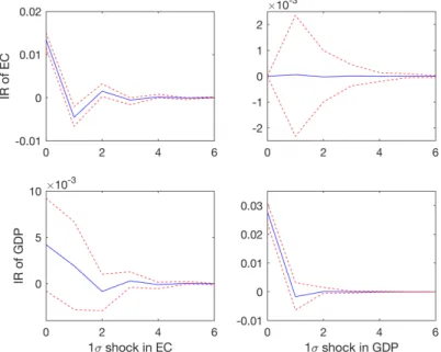
Figure : Impulse Response Functions based on the VAR( ) model of quarterly Electricity Consumption (EC) and quarterly GDP

(23)

Figure reports the analysis on the impulse responses of quarterly electricity consumption (EC) and GDP using a conventional VAR model. As VAR model requires all the variables in the model to be in the same frequency, I aligned monthly electricity consumption downward to treat it as a quarterly variable. As it can be seen from this figure, neither a one-standard deviation shock in quarterly electricity consumption nor a one-standard deviation shock in GDP generate statistically significant results in terms of the impulse responses of GDP and quarterly electricity consumption, respectively.

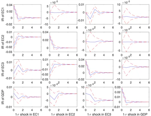
Figure : Impulse Response Functions based on the MF-VAR( ) model of monthly Electricity Consumptions (EC1, EC2, EC3) and quarterly GDP

In Figure , however, I used the MF-VAR model to test the same relationship but with monthly electricity consumption and quarterly GDP data without do-ing any alignment. For notational convenience I use EC1 instead of EC3

t≠2/3

which is the electricity consumption of the first month of each quarter. Simi-larly, I indicate the electricity consumption of the second month of each

(24)

quar-ter EC3

t≠1/3, and the electricity consumption of the third month of each quarter

EC_t3_≠0/3 with EC2 and EC3, respectively. The last column of Figure sug-gests that a shock in GDP does not affect any of the monthly electricity con-sumptions in a statistically significant fashion. However, the last row of the fig-ure reports that a shock in EC3 increases GDP growth in a statistically signif-icant fashion. Hence, an increase in electricity consumption causes an increase in GDP lending support for the growth hypothesis. This result is parallel to the one found by Altinay and Karagol ( ); using - data, they too find a unidirectional causality running from electricity consumption to income for Turkey.

Here, the reason behind the difference between the two impulse responses may arise from the possibility that Figure may suffer from the consequences of ignoring the availability of high frequency data. For this reason, the impulse responses of the MF-VAR model has a greater explanatory power than the im-pulse responses of the quarterly VAR (lower type-II error).

Next, I re-perform the analysis by adding an additional quarterly variable to the MF-VAR specification. There are two reasons to adding this second low frequency variable. Firstly, I want to see if monthly electricity consumptions affect these added variables differently than how they affect GDP. Secondly, I want to analyze if a shock in the added variable effects electricity consumption differently compared to a shock in GDP.

Figure to Figure reports the impulse responses of our MF-VAR model with added variables. From Figure , I report the impulse response esti-mates that concern the added variables and monthly electricity consump-tions only because the rest is almost identical to Figure . Based on this, the first columns of Figure to report how a one-standard deviation shock in EC1, EC2, EC3 affects the added variable. The second column of these

(25)

fig-ures, on the other hand, report how a one-standard deviation shock in the added variables affects the monthly electricity consumptions. The added vari-ables from Figure to are based on the expenditure approach of GDP calcu-lation that includes Private Consumption Expenditure; Government Spending; Investment; Exports; and Imports. The added variables From Figure to , on the other hand, are based on the production approach of GDP calculation and include Construction Sector; Industrial Sector; Manufacturing Industry; Service; and Agricultural Sector outputs.

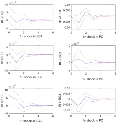
Figure : Impulse Response Functions based on the MF-VAR( ) model of monthly Electricity Consumptions (EC1, EC2, EC3) and quarterly Private Consumption (P C)

Figure reports the impulse responses of Private Consumption Expenditure relative to GDP and monthly electricity consumptions. The first column of Figure reports that a one-standard deviation shock in EC1 and EC2 do not generate statistically significant results. However, a shock in EC3 increases Private Consumption Expenditure more than it increases GDP in a

(26)

statisti-cally significant fashion. The second column on the other hand, reports that a one-standard deviation shock in Private Consumption relative to GDP in-creases only EC1 in the second period in a statistically significant fashion.

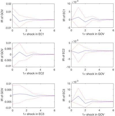
Figure : Impulse Response Functions based on the MF-VAR( ) model of monthly Electricity Consumptions (EC1, EC2, EC3) and quarterly Government Spending (GOV )

Repeating the same exercise with Government Spending as the second low frequency variable that is placed after GDP, Figure reports that impulse responses of Government Spending to a one-standard deviations shock in monthly electricity consumption and the impulse responses of monthly elec-tricity consumption to a one-standard deviation shock in Government Spending relative to GDP are not statistically significant.

(27)

Figure : Impulse Response Functions based on the MF-VAR( ) model of monthly Electricity Consumptions (EC1, EC2, EC3) and quarterly Investment (INV )

The first column of Figure reports that a one-standard deviation shock in only EC3 among the three monthly electricity consumptions affect Investment relative to GDP in a statistically significant fashion. It increases Investment more than it increases GDP as it can be seen for the first period. This im-plies that generating more electricity to Investment will have a positive affect in GDP. The second column on the other hand, reports that a one-standard deviation shock in Investment relative to GDP does not generate statistically significant impulse responses of monthly electricity consumptions.

(28)

Figure : Impulse Response Functions based on the MF-VAR( ) model of monthly Electricity Consumptions (EC1, EC2, EC3) and quarterly Exports (EX)

Figure : Impulse Response Functions based on the MF-VAR( ) model of monthly Electricity Consumptions (EC1, EC2, EC3) and quarterly Imports (IM)

(29)

Replacing the second low frequency variable with Exports, Figure reports that neither of the responses are statistically significant. However, when I take Imports relative to GDP as the second low frequency variable it is evident that a one-standard deviation shock in EC3, which is the only shock that generates statistically significant results in Figure , increases Imports more than it in-creases GDP. The second column of both figures show that neither a shock in Exports nor Imports relative to GDP have a statistically significant affect on monthly electricity consumptions.

Figure : Impulse Response Functions based on the MF-VAR( ) model of monthly Electricity Consumptions (EC1, EC2, EC3) and quarterly Construction Sector output (CONS)

Figure on the other hand reports the impulse responses of the monthly elec-tricity consumptions and Construction Sector output relative to GDP. The first column reports a shock in EC1 and EC2 does not affect Construction Sector output relative to GDP in a statistically significant fashion. However, a shock in EC3 increases Construction Sector output more than it increases GDP in

(30)

a statistically significant way. For the impulse responses of the electricity con-sumption to a one-standard deviation of the added variables, I was not able to find any statistically significant results for Figures to .

Figure : Impulse Response Functions based on the MF-VAR( ) model of monthly Electricity Consumptions (EC1, EC2, EC3) and quarterly Manufacturing Sector output (MAN)

Figure shows the impulse response functions with the Manufacturing Indus-try output, (MAN) as the second low frequency variable. The first column of the figure reports that the response of MAN relative to GDP to a shock in EC2 is not statistically significant. However, a shock in EC1 and EC3 in-creases Manufacturing Sector output relative to GDP in a statistically signif-icant fashion. Hence, an increase in electricity consumption increases manufac-turing sector output more than it increases GDP.

(31)

Figure : Impulse Response Functions based on the MF-VAR( ) model of monthly Electricity Consumptions (EC1, EC2, EC3) and quarterly Industrial Sector output (IND)

Replacing the last variable in the model with Industrial Sector output, (IND) the first column of Figure reports the impulse responses of industrial sec-tor output relative to GDP to a shock in monthly electricity consumptions. Based on the Distribution of net electricity consumption by sectors statistics of TUIK, the sector that consumes electricity the most is the Industrial sector. For this reason, I expect its relation with electricity consumption to be strong. Based on the first column of Figure it is evident that a shock in EC2 does not generate statistically significant results. However, a shock in EC1 and EC3 increases Industrial Sector output relative to GDP in a statistically sig-nificant fashion. This in turn means that an increase in electricity consumption increases Industrial Sector output more than it increases GDP.

(32)

Figure : Impulse Response Functions based on the MF-VAR( ) model of monthly Electricity Consumptions (EC1, EC2, EC3) and quarterly Service Sector output (SERV )

In Figure , I take Service Sector output as the second low frequency variable. Looking at the first column of this figure, we see that shocks to EC1 and EC3 increases Service Sector output more than they increase GDP. A shock in EC2 does not generate any statistically significant impulse responses in the added variable.

(33)

Figure : Impulse Response Functions based on the MF-VAR( ) model of monthly Electricity Consumptions (EC1, EC2, EC3) and quarterly Agricultural Sector output (AG)

Figure reports the impulse responses of monthly electricity consumption and Agricultural Sector output relative to GDP. Different from the previous results, this figure reports that in the first period an increase in EC2 increases Agri-cultural sector output less than it increases GDP which is the only statistically significant result in this table.

(34)

CHAPTER

CONCLUSION

In this study, I investigated the relationship between electricity consumption and GDP growth as well as the relationship between electricity consumption and relative growth of GDP’s components to GDP for the Turkish economy. When I used a conventional quarterly VAR model, I could not find a statis-tically significant relationship between quarterly electricity consumption and quarterly GDP growth with the impulse response analysis. However, when I adopted the Mixed Frequency VAR specification with monthly electricity con-sumption and quarterly GDP I found that an increase in electricity consump-tion increases GDP growth.

Continuing to use MF-VAR model but with an added low frequency variable, I found that an increase in electricity consumption increases Private Consump-tion, Investment, Imports more than a positive shock in electricity consump-tion increases GDP. Similarly, an increase in electricity consumpconsump-tion increases Construction sector output, Manufacturing sector output, Industrial sector out-put and Service sector outout-put more than a positive shock in electricity con-sumption increases GDP. Different from these results, I found that an increase in electricity consumption increases Agricultural sector output less than it in-creases GDP. One of the reasons behind this difference may be due to the fact that Construction, Manufacturing, Industrial and Service sectors are more

(35)

cap-ital intensive when compared to the Agricultural sector. Hence, their electricity consumptions are higher. Second reason may be the farmers in Turkey stick to more traditional tools instead of using electricity dependent agricultural ma-chines to improve crops, livestock, fishery and forestry or they use diesel fuel dependent machines rather than electricity dependent ones in the Agricultural sector especially when the Turkish government gives subsidies to this sector for diesel fuel from time to time.

Looking at the effect of a shock in the added variable on electricity consump-tion, on the other hand, I could not find a statistically significant result ex-cept for the effect of a shock in Private Consumption on electricity consump-tion. The estimation suggests that a positive shock in Private Consumption increases electricity consumption.

(36)

REFERENCES

Abokyi, E., Appiah-Konadu, P., Sikayena, I., & Oteng-Abayie, E. F. ( ). Consumption of electricity and industrial growth in the case of Ghana. Jour-nal of Energy, , - . doi: . / /

Altinay, G., & Karagol, E. ( ). Electricity consumption and economic growth: Evidence from Turkey. Energy Economics, ( ), - . doi: https://doi.org/ . /j.eneco. . .

Apergis, N., & Payne, J. E. ( ). Energy consumption and economic growth in Central America: Evidence from a panel cointegration and error correc-tion model. Energy Economics, ( ), - . doi: https://doi.org/ . / j.eneco. . .

Borozan, D. ( ). Exploring the relationship between energy consumption and GDP: Evidence from Croatia. Energy Policy, , - . doi: https:// doi.org/ . /j.enpol. . .

Chauvet, M., Götz, T. B., & Hecq, A. ( ). Realized volatility and business cycle fluctuations: A mixed-frequency var approach..

Csereklyei, Z., & Humer, S. ( ). Modelling primary energy consumption under model uncertainty. (Department of Economics Working Paper Series,

. WU Vienna University of Economics and Business, Vienna)

Danmaraya, I. A., & Hassan, S. ( ). Electricity consumption and manufac-turing sector productivity in Nigeria: An autogressive distributed lag-bounds testing approach. International Journal of Energy Economics and Policy,

( ), - .

Ghosh, S. ( ). Electricity consumption and economic growth in India. Energy Policy, ( ), - . doi: https://doi.org/ . /S - ( )

-Ghysels, E. ( ). Macroeconomics and the reality of mixed frequency data. Journal of Econometrics, ( ), - . doi: https://doi.org/ . / j.jeconom. . .

Götz, T. B., Hecq, A., & Smeekes, S. ( ). Testing for Granger causality in large mixed frequency VARs. Journal of Econometrics, ( ), - . doi:

(37)

https://doi.org/ . /j.jeconom. . .

Hamzacebi, C. ( ). Forecasting of Turkey’s net electricity energy con-sumption on sectoral bases. Energy Policy, ( ), - . doi: https:// doi.org/ . /j.enpol. . .

Jamil, F., & Ahmad, E. ( ). The relationship between electricity consump-tion, electricity prices and GDP in Pakistan. Energy Policy, ( ),

-. doi: https://doi-.org/ -. /j.enpol. . .

Jumbe, C. B. L. ( ). Cointegration and causality between electricity con-sumption and GDP: empirical evidence from Malawi. Energy Economics,

( ), - . doi: https://doi.org/ . /S - ( )

-Kermani, F. I., Ghasemi, M., & Abbasi, F. ( ). Industrialization, electricity consumption and co emissions in Iran. International Journal of Innovation and Applied Studies, , - . doi: . /s - - -z

Kouakou, A. K. ( ). Economic growth and electricity consumption in Cote d’Ivoire: Evidence from time series analysis. Energy Policy, ( ),

Kwakwa, P. ( ). Disaggregated energy consumption and economic growth in Ghana. International Journal of Energy Economics and Policy, , - . Lean, H. H., & Smyth, R. ( ). On the dynamics of aggregate output,

electricity consumption and exports in Malaysia: Evidence from multi-variate Granger causality tests. Applied Energy, ( ), - . doi: https://doi.org/ . /j.apenergy. . .

Mawejje, J., & Mawejje, N. D. ( ). Electricity consumption and sectoral output in Uganda: an empirical investigation. Journal of Economic Struc-tures, ( ), - . doi: . /s - -

-Narayan, P. K., & Singh, B. ( ). The electricity consumption and GDP nexus for the Fiji Islands. Energy Economics, ( ), - . doi: https:// doi.org/ . /j.eneco. . .

Narayan, P. K., & Smyth, R. ( ). Electricity consumption, employment and real income in Australia evidence from multivariate Granger causality tests. Energy Policy, ( ), - . doi: ttps://doi.org/ . /j.enpol

. . .

Odhiambo, N. M. ( ). Electricity consumption and economic growth in South Africa: A trivariate causality test. Energy Economics, ( ), - . doi: https://doi.org/ . /j.eneco. . .

Payne, J. E. ( a). A survey of the electricity consumption-growth lit-erature. Applied Energy, ( ), - . doi: https://doi.org/ . / j.apenergy. . .

(38)

Payne, J. E. ( b). Survey of the international evidence on the causal re-lationship between energy consumption and growth. Journal of Economic Studies, ( ), - . doi: . /

Pereira, J., & Matheson, T. ( ). Fiscal multipliers for Brazil. (IMF Work-ing Paper No. / )

Qian, H. ( ). Vector autoregression with mixed frequency data (MPRA Paper). University Library of Munich, Germany. Retrieved from https:// EconPapers.repec.org/RePEc:pra:mprapa:

Shahbaz, M., Uddin, G. S., Rehman, I. U., & Imran, K. ( ). Industrializa-tion, electricity consumption and co emissions in Bangladesh. Renewable and Sustainable Energy Reviews, , - . doi: https://doi.org/ . / j.rser. . .

Shiu, A., & Lam, P. L. ( ). Electricity consumption and economic growth in China. Energy Policy, ( ), - . doi: https://doi.org/ . /S

- ( )

-Strongin, S. ( ). The identification of monetary policy disturbances ex-plaining the liquidity puzzle. Journal of Monetary Economics, ( ),

-. Retrieved from https://EconPapers-.repec-.org/RePEc:eee:moneco:v: : y: :i: :p:

-Tang, C. F., & Shahbaz, M. ( ). Sectoral analysis of the causal relationship between electricity consumption and real output in Pakistan. Energy Policy,

, - . doi: https://doi.org/ . /j.enpol. . .

TEIAS, Turkish Electricity Transmission Corporation. ( ). Electric-ity generation and transmission statistics of Turkey. (Retrieved from https://www.teias.gov.tr/tr)

TUIK, T. S. I. (n.d.). Turkish foreign trade by years. (Retrieved from http://www.tuik.gov.tr/PreTablo.do?alt_id= )

Wolde-Rufael, Y. ( ). Electricity consumption and economic growth: a time series experience for African countries. Energy Policy, ( ),

World Bank. (n.d.). GDP per capita growth (annual %). (Retrieved from https://data.worldbank.org/indicator/NY.GDP.PCAP.KD.ZG?view=chart) Yoo, S. H. ( ). Electricity consumption and economic growth: evidence

from Korea. Energy Policy, ( ), - . doi: https://doi.org/ . / j.enpol. . .

Yoo, S. H., & Kim, Y. ( ). Electricity generation and economic growth in Indonesia. Energy, ( ), - . doi: https://doi.org/ . /j.energy