APPLICATIONS
a thesis
submitted to the department of electrical and
electronics engineering
and the institute of engineering and science
of bilkent university
in partial fulfillment of the requirements
for the degree of
master of science
By
Berkan D¨ulek
November, 2005
I certify that I have read this thesis and that in my opinion it is fully adequate, in scope and in quality, as a thesis for the degree of Master of Science.
Prof. Dr. Ahmet Enis C¸ etin(Supervisor)
I certify that I have read this thesis and that in my opinion it is fully adequate, in scope and in quality, as a thesis for the degree of Master of Science.
Prof. Dr. ¨Ozg¨ur Ulusoy
I certify that I have read this thesis and that in my opinion it is fully adequate, in scope and in quality, as a thesis for the degree of Master of Science.
Asst. Prof. Dr. U˘gur G¨ud¨ukbay
Approved for the Institute of Engineering and Science:
Prof. Dr. Mehmet B. Baray
Director of the Institute Engineering and Science ii
FOR AGRICULTURAL APPLICATIONS
Berkan D¨ulek
M.S. in Electrical and Electronics Engineering Supervisor: Prof. Dr. Ahmet Enis C¸ etin
November, 2005
Medical studies indicate that acrylamide causes cancer in animals and certain doses of acrylamide are toxic to the nervous system of both animals and humans. Acrylamide is produced in carbohydrate foods prepared at high temperatures such as fried potatoes. For this reason, it is crucial for human health to quanti-tatively measure the amount of acrylamide formed as a result of prolonged cook-ing at high temperatures. In this thesis, a correlation is demonstrated between measured acrylamide concentrations and NABY (Normalized Area of Brownish Yellow regions) values estimated from surface color properties of fried potato im-ages using a modified form of the k-means algorithm. Same method is used to estimate acrylamide levels of roasted coffee beans. The proposed method seems to be a promising approach for the estimation of acrylamide levels and can find applications in industrial systems.
The quality and price of hazelnuts are mainly determined by the ratio of shell weight to kernel weight. Due to a number of physiological and physical disorders, hazelnuts may grow without fully developed kernels. We previously proposed a prototype system which detects empty hazelnuts by dropping them onto a steel plate and processing the acoustic signal generated when kernels hit the plate. In that study, feature vectors describing time and frequency nature of the impact sound were extracted from the acoustic signal and classified using Support Vector Machines. In the second part of this thesis, a feature domain post-processing method based on vector median/mean filtering is shown to further increase these classification results.
Keywords: Acrylamide, fried potatoes, coffee, k-means, image analysis, color,
seg-mentation, median/mean filtering, hazelnuts, acoustics, classification, aflatoxin. iii
¨
OZET
TARIMSAL UYGULAMALAR ˙IC
¸ ˙IN S˙INYAL VE ˙IMGE
˙IS¸LEME ALGOR˙ITMALARI
Berkan D¨ulek
Elektrik ve Elektronik M¨uhendisli˘gi, Y¨uksek Lisans Tez Y¨oneticisi: Prof. Dr. Ahmet Enis C¸ etin
Kasım, 2005
Tıbbi ara¸stırmalar akrilamidin hayvanlarda kansere neden oldu˘gunu ve belirli dozlarının hayvan ve insan sinir sistemleri ¨uzerinde toksik etkisinin bulundu˘gunu g¨ostermi¸stir. Patates kızartması gibi y¨uksek sıcaklıklarda hazırlanan karbon-hidratlı besinlerde akrilamide rastlanılmaktadır. Dolayısıyla besinlerin y¨uksek sıcaklıklarda uzun s¨ureli pi¸sirilmesi sonucunda olu¸san akrilamid miktarının ni-cel olarak ¨ol¸c¨ulebilmesi insan sa˘glı˘gı a¸cısından b¨uy¨uk ¨onem ta¸sımaktadır. Bu tezde, k-ortalama algoritmasına dayanan bir y¨ontem geli¸stirilerek deneysel olarak ¨ol¸c¨ulm¨u¸s akrilamid konsantrasyonları ile patates kızartması ve kahve imgelerinin y¨uzeysel renk analizinden tahmin edilen NABY (Kahverengimsi Sarı B¨olgelerin Standartla¸stırılmı¸s Alanı) de˘gerleri arasında bir ilintinin varlı˘gı g¨osterilmektedir.
¨
Onerilen y¨ontem akrilamid seviyelerinin sa˘glıklı tahmini i¸cin umut verici bir yakla¸sım olarak g¨oz¨ukmekte ve end¨ustriyel alanda uygulanabilirli˘gi bulunmak-tadır. Paketleme hatlarına kameralar yerle¸stirilerek patates kızartmalarına ait imgeler ger¸cek-zamanda analiz edilebilir ve y¨uksek NABY de˘gerlerine sahip olan-lar ayrı¸stırılabilir.
Fındıkların kalite ve fiyatlarının belirlenmesinde temel unsur ¸cekirdek a˘gırlı˘gının ¸cekirdek i¸ci a˘gırlı˘ga oranıdır. Susuzluk, besleyici ¨o˘gelerin azlı˘gı ve kurtlanma gibi fizyolojik ve fiziksel sebeplerle fındıkların i¸ci tam olarak geli¸semeyebilir. Dolayısıyla bo¸s ve dolu fındıkların g¨uvenilir bir ¸sekilde otomatik olarak ayrı¸stırılabilmesi b¨uy¨uk ¨onem ta¸sımaktadır. Onceki bir ¸calı¸smamızda¨ fındıkları ¸celik bir plakanın ¨uzerine atıp ¸carpma esnasında ortaya ¸cıkan akustik sinyali i¸sleyerek bo¸s fındıkları bulan bir sistem ¨onermi¸stik. C¸ arpma sesinin za-man ve frekans b¨olgesine ait ¨ozelliklerini a¸cıklayan ¨oznitelik vekt¨orleri ¸cıkarılmı¸s ve Destek Vekt¨or Makineleri kullanılarak sınıflandırma yapılmı¸stı. Bu tezin
ikinci kısmında, vekt¨or ortanca/ortalama temelli s¨uzmeye dayanan bir ¨oznitelik b¨olgesi art-i¸sleme y¨ontemi tasarlanarak fındıklara ait ayrı¸stırma sonu¸clarının arttı˘gı g¨osterilmektedir.
Anahtar s¨ozc¨ukler : Akrilamid, patates kızartması, kahve, k-ortalama, imge
ana-lizi, renk, b¨ol¨utleme, ortanca/ortalama s¨uzgeci, fındık, akustik, sınıflandırma, aflatoksin.
Acknowledgement
I would like to express my deep gratitude to my supervisor Prof. Dr. Ahmet Enis C¸ etin for his instructive comments and constant support throughout this study.
I would like to express my special thanks to Prof. Dr. ¨Ozg¨ur Ulusoy and Asst. Prof. Dr. U˘gur G¨ud¨ukbay for showing keen interest to the subject matter and accepting to read and review the thesis.
I would also like to thank Assoc. Prof. Dr. Vural G¨okmen and Asst. Prof. Dr. Selim Aksoy for many helpful suggestions and discussions.
1 Introduction 1
1.1 Image Analysis for Acrylamide Formation . . . 1
1.1.1 Motivation . . . 1
1.1.2 Related Work . . . 2
1.2 Detection of Empty Hazelnuts using Impact Acoustics . . . 4
1.2.1 Motivation . . . 4
1.2.2 Related Work . . . 5
1.3 Organization of the Thesis . . . 6
2 Modified K-means based Classification 7 2.1 K-means Clustering . . . . 7
2.1.1 Major Drawbacks of the K-means Algorithm . . . . 10
2.1.1.1 Information Criterion Scoring for Estimation of the Optimal Number of Clusters . . . 10
2.1.2 Computational Complexity of the Algorithm . . . 12
CONTENTS viii
2.1.3 Improvement of the Algorithm . . . 12
2.1.3.1 Simulated Annealing . . . 13
2.1.3.2 Fuzzy K-means . . . . 14
2.2 Our K-means based Classification Algorithm . . . . 14
2.2.1 Properties of the Method and Examples . . . 17
2.2.2 Performance Comparison . . . 23
3 Image Analysis of Potato Chips 28 3.1 Modeling Acrylamide Formation using Image Analysis . . . 29
3.2 Acrylamide Analysis using CIE a∗ Parameter . . . . 30
3.2.1 Color Spaces . . . 30
3.2.2 Color Differences and CIE L∗a∗b∗ Color Space . . . . 32
3.2.3 Conversion from CIE XYZ to CIE L∗a∗b∗ . . . . 33
3.2.4 Practical Issues . . . 33
3.2.5 Results and Discussion . . . 34
3.3 K-means Clustering based Segmentation for Acrylamide Analysis in Potato Chip Images . . . 36
3.3.1 Selected Features . . . 37
3.3.2 Classification Results . . . 40
4 Image Analysis of Coffee Beans 42
5.1 Experimental Setup and Dataset . . . 48
5.2 Signal Processing . . . 48
5.2.1 Feature Extraction . . . 49
5.2.1.1 Time Domain Signal Modeling . . . 49
5.2.1.2 Short Time Variances in Frames of Data . . . 50
5.2.1.3 Extrema in Short Time Windows . . . 51
5.2.1.4 Frequency Domain Processing . . . 51
5.2.1.5 Line Spectral Frequencies . . . 52
5.3 Mean and Median Filtering Based Post-Processing . . . 53
5.3.1 Algorithm . . . 53
5.3.2 Performance Analysis . . . 55
5.4 Support Vector Machine Classifier . . . 55
5.5 Classification and Comparison of Results . . . 57
6 Conclusions 59
List of Figures
1.1 Relation of acrylamide concentration to CIE a∗ parameter . . . . 4
1.2 Experimental apparatus for collecting acoustic emissions . . . 5
2.1 Effect of initial point selection on the performance of k-means al-gorithm . . . 9
2.2 Effect of increasing k on our modified k-means algorithm . . . . . 19
2.3 Effect of increasing T1 on our modified k-means algorithm . . . . 20
2.4 Effect of brute force searching on our modified k-means algorithm 21 2.5 Effect of different brute force searching methods on our modified k-means algorithm . . . . 22
2.6 Performance comparison on Lithuanian dataset . . . 25
2.7 Performance comparison on banana-shaped dataset-1 . . . 26
2.8 Performance comparison on banana-shaped dataset-2 . . . 27
3.1 (a) Original fried potato chip image with selected regions, and (b) Result of our segmentation algorithm . . . 30
3.2 Images of potato chips used for acrylamide analysis . . . 34 x
3.3 Relation of acrylamide concentration to estimated CIE a∗ parameter 36
3.4 Potato regions used in feature distribution and autocovariance
es-timation plots . . . 38
3.5 Distribution of acrylamide features in normalized RGB space . . . 38
3.6 Row-wise unbiased autocovariance estimates from normalized red pixels . . . 39
3.7 Change of acrylamide level and NABY value in potato chips during frying at 170◦C. . . . 41
3.8 Correlation between acrylamide level and NABY value in potato chips . . . 41
4.1 Coffee images used for acrylamide analysis . . . 43
4.2 Frequency response of the low-pass filter . . . 44
4.3 (a) Original coffee image and (b) Segmented coffee image . . . 44
4.4 Change of acrylamide level and NABY value in coffee images . . . 45
5.1 Typical impact sound signals from an empty hazelnut and a full hazelnut . . . 49
5.2 Average variances from short time windows . . . 50
5.3 Frequency spectra magnitudes of empty and full hazelnuts . . . . 51
List of Tables
2.1 Effect of increasing k on classification performance . . . . 19 2.2 Effect of increasing T1 on classification performance . . . 20
2.3 Effect of brute force searching on the representation of training set 21 2.4 Effect of other brute force searching methods on the representation
of training set . . . 22 2.5 Performance comparison of our modified k-means algorithm with
other well-known classifiers . . . 23 3.1 Measured acrylamide concentration, measured and estimated CIE
a∗ values for potato chips . . . . 35
3.2 Measured acrylamide concentration and estimated NABY value for potato chips . . . 40 4.1 Low-pass filter coefficients . . . 43 4.2 Measured acrylamide concentration and estimated NABY value
for coffee roasted at 150◦C . . . . 46
4.3 Measured acrylamide concentration and estimated NABY value for coffee roasted at 200◦C . . . . 46
4.4 Measured acrylamide concentration and estimated NABY value for coffee roasted at 225◦C . . . . 46
5.1 Classification results obtained for banana shaped classes . . . 55 5.2 Classification results with/without post-processing . . . 58
Chapter 1
Introduction
With the development of fast and reliable computer technologies, digital signal and image processing algorithms have found vast application areas such as au-tomation, defense, agriculture, health and robotics. In this thesis, we focus on two specific agricultural applications and propose algorithms based on signal and image processing techniques. The first application is the estimation of acrylamide levels in fried potato chips and roasted coffee beans using digital color images. The second is the detection of empty hazelnuts from fully developed nuts using impact acoustics. Following sections explain the motivations behind these in-triguing applications, summarize the previous work and conclude with an outline of the organization of this thesis.
1.1
Image Analysis for Acrylamide Formation
1.1.1
Motivation
Acrylamide is a chemical that is used to make polyacrilamide materials. Poly-acrylamide is used in the treatment of drinking-water and waste water to remove particles and other impurities. It is also used to make glues, paper and cosmetics. Polyacrylamide materials contain very small amounts of acrylamide. Acrylamide
is also used in the construction of dam foundations and tunnels, and appears to be produced in some foods prepared at high temperatures such as fried potatoes. The levels of acrylamide found in some foods are much higher than the levels rec-ommended for drinking-water, or levels expected to occur as a result of contact between food and food packing (from paper) or use of cosmetics. The highest levels found so far are in starchy foods (potato and cereal products).1
Acrylamide formation was found to occur during the browning process by Maillard reaction of reducing sugars with asparagine at temperatures above 120◦C [1, 2, 3, 4]. Colored products are also formed in foods during heating
as a result of Maillard reaction [5, 6, 7]. These brown polymers have significant effect on the quality of food, because color is an important food attribute and a key factor in consumer acceptance. Mechanism of the formation of brown color is not fully understood yet [8].
The problem with acrylamide is that it is known to cause cancer in animals. Also, certain doses of acrylamide are toxic to the nervous system of both animals and humans. For this reason, it is crucial for human health to quantitatively measure the amount of acrylamide formed as a result of prolonged cooking at high temperatures. If a correlation is demonstrated between acrylamide concentration and surface color properties of thermally processed food images, a machine vision based system can be designed to remove those products having high levels of acrylamide from a packaging line by means of a surface image analysis.
1.1.2
Related Work
Since color can easily be measured, it may be used as an indicator of Maillard reaction products like acrylamide. Color of foods is usually measured in L∗a∗b∗
units which is an international standard for color measurements, adopted by the Commission Internationale d’Eclairage (CIE) in 1976. L∗ is the luminance or
lightness component (black to white), and parameters a∗ (from green to red) and
1More information about acrylamide is available on http://www.who.int/foodsafety/
CHAPTER 1. INTRODUCTION 3
b∗ (from blue to yellow) are the two chromatic components [9]. Amrein et al.
re-ported a significant correlation between the L∗ values and the acrylamide content
during baking at 180◦C [10]. Surdyk et al. also reported a highly significant
cor-relation between color and acrylamide content in bread crust during baking [11]. Pedrechi et al. reported that L∗ and b∗ values did not show considerable changes
as those shown by a∗ during frying of potato chips [6]. A linear correlation was
found between the acrylamide concentration and the color of potato chips repre-sented by the redness component a* at temperatures of 120, 150 and 180◦C for
up to 5 minutes of frying. However, the effect of prolonged frying on acrylamide concentration and color was not mentioned by these researchers. Taubert et al. investigated the relation between the level of surface browning and acrylamide concentration of French fries with linear regression. They reported that there could be a close correlation for small-surface material being fried [12]. A some-what less close correlation was observed for intermediate-surface material, while no correlation was observed for large-surface material.
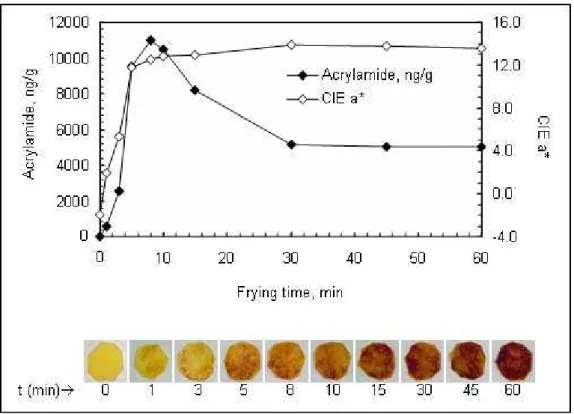
Although these findings suggest that surface color may be correlated with acrylamide concentration in thermally processed foods, the measurement of sur-face image and its color properties need to be investigated in more detail to establish a useful correlation. As illustrated in Figure 1.1, the amount of mea-sured acrylamide increases rapidly at the onset of frying, reaching an apparent maximum concentration of 10963 ng/g. However, the acrylamide concentration in potato chips decreases exponentially as the time passes. These results suggest that acrylamide forms as an intermediate product during Maillard reaction and its concentration begins to decrease as the rate of degradation exceeds the rate of formation during heating. Although the rapid increase is conveniently modeled by CIE a∗ parameter, the exponential fall is not captured. The study also shows
that CIE L∗ and b∗ values decrease exponentially during frying at 170◦C and
Figure 1.1: Change of acrylamide concentration and CIE redness parameter a∗
in potato chips during frying at 170◦C
1.2
Detection of Empty Hazelnuts using Impact
Acoustics
1.2.1
Motivation
The quality and price of hazelnuts is mainly determined by the ratio of shell weight to kernel weight. Due to physiological disorders such as plant stress, dehydration and lack of nutrients, hazelnuts may grow without fully developed kernels. Physical disorders such as insect infestation also prevent hazelnuts to develop into a healthy form by intervening the maturation process. It is usually the case that empty hazelnuts and nuts with undeveloped kernels contain a cancer causing material, called aflatoxin. Currently, pneumatic devices are employed to segregate between empty and full hazelnuts. However, these devices suffer from
CHAPTER 1. INTRODUCTION 5
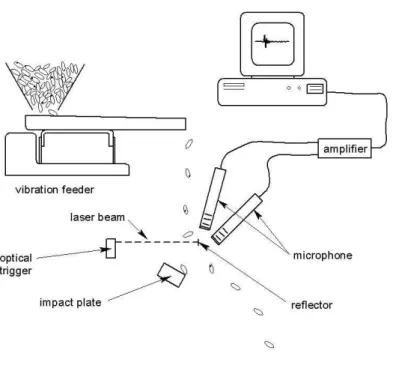
Figure 1.2: Schematic of experimental apparatus for collecting acoustic emissions from hazelnuts
high classification error rates. Therefore, it becomes a necessity both industrially and in terms of food safety to provide a reliable separation between these two types of product in an autonomous manner.
1.2.2
Related Work
Previously, a high-throughput (20-40 nuts/second), low-cost acoustical prototype system was developed to separate pistachio nuts with closed shells from those with cracked shells in real time [13, 14, 15]. A similar system was proposed to detect empty hazelnuts by dropping them onto a steel plate and processing the acoustic signal generated when the kernel hits the plate [16]. An air valve can be used to separate detected empty hazelnuts from the process stream. The schematic diagram of the system is shown in Figure 1.2. The proposed system works reliably in a food processing environment with little maintenance or skill required to operate. In addition, signal processing part can be carried out in an ordinary PC with 44kHz sound sampling capability.
1.3
Organization of the Thesis
Chapter 2 develops a modified version of the well-known k-means clustering al-gorithm [17, 18] so that it can be used effectively in any supervised classification framework. A performance analysis is carried out to compare the results with some other state-of-the-art classification techniques such as Gaussian Mixture Modeling, Support Vector Machines, Back-Propagation Neural Networks and K-Nearest Neighbors [19].
In Chapter 3 and 4, the proposed method is applied to estimate acrylamide levels in digital color images of fried potato chips and roasted coffee beans, re-spectively. The relation between CIE a∗ values and acrylamide levels of potato
chips is investigated and it is observed that it is hard to define specific regions in the range of a∗ values that point to acrylamide formation. A new method
based on the segmentation of fried potato images into three regions is devised. Normalized-RGB color values are used as features for the segmentation of acry-lamide contaminated areas in digital images. The changes of acryacry-lamide levels and estimated values are tabulated and shown to follow almost the same trend. We also demonstrate that autocovariance estimates can be incorporated as addi-tional statistical features into the feature set of fried potato images.
In Chapter 5, a feature domain post-processing method is developed to in-crease performance in the separation of empty hazelnuts from fully developed nuts by impact acoustics. The idea is inspired from the well-known median filter-ing approach. In addition to median filterfilter-ing based post-processfilter-ing, the results of an averaging filter are also examined.
The last chapter concludes the thesis with an elaborate summary of the results obtained in the previous chapters.
Chapter 2
Modified K-means based
Classification
In this chapter, we provide a modification for the k-means algorithm which makes it more suitable for classifying data in a supervised manner within a training-followed-by-testing framework. K-means clustering algorithm [17, 18] is chosen because of its simplicity, high performance and fast implementation properties. In the following sections, we present a summary of the k-means clustering al-gorithm, our contribution to this alal-gorithm, application of our method to some popular classification datasets and performance comparison with other widely used classification methods. The proposed method is generic in the sense that it can be applied to any classification dataset without much modification.
2.1
K-means Clustering
K-means clustering is one of the simplest unsupervised learning algorithms that
is adopted to many problem domains as a result of its simple computation and accelerated convergence. It is also called Vector Quantization (VQ) in digital waveform coding literature [20]. It is a very popular method listed under the class of iterative optimization procedures. Given a dataset, this procedure provides an
easy and simple way to partition the observation vectors in the dataset into k mutually exclusive clusters. It is computationally efficient and gives good results if the clusters are compact, hyperspherical in shape and well-separated in feature space. The main idea in k-means is to arrange the partitions in such a way that objects belonging to a certain cluster are as close to each other as possible and as far from the objects in other clusters as possible. Each object in the dataset is identified with the index of the cluster to which it belongs and the centroid for each cluster is the point to which the sum of distances from all objects in that cluster is minimized.
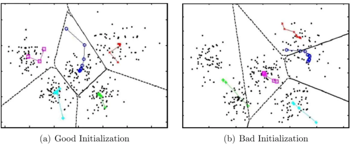
Fixing the number of clusters a priori, the algorithm starts with the selection of k initial cluster centroids inside the space spanned by the observation vectors. The wise thing to do at this point is to select these initial points in such a way that they are separated as much as possible from each other inside the cloud of data points. At the next step, all points in the dataset are assigned to their nearest cluster centers with respect to a predefined distance measure. After all the points are processed, k new cluster centroids are calculated using the cluster bindings obtained in the previous step. Then a new iteration is initiated by reassigning points to their nearest cluster centroids resulting from the last iteration. Each iteration consists of these two consecutive steps of cluster assignment and centroid calculation. With this iterative approach, k centroids change their location step by step until no more changes are possible as illustrated in Figure 2.1(a). This results in the minimization of a criterion function, in this case the sum of point-to-centroid distances, summed over all k clusters. Depending on the kind of data being clustered, an educated selection can be made among a number of distance measures such as Minkowski, Euclidean, city-block and cosine distances.
Suppose that a dataset of n patterns is partitioned into k clusters D1, . . . , Dk
at any stage during the iterative procedure. Let ni be the number of samples
assigned to Di and let mi be the mean of those samples:
mi = 1 ni X x∈Di x
CHAPTER 2. MODIFIED K-MEANS BASED CLASSIFICATION 9
(a) Good Initialization (b) Bad Initialization
Figure 2.1: Effect of initial point selection on the performance of k-means al-gorithm. Here the same dataset is partitioned into five clusters; (a) yields the desired clustering while (b) gets trapped in a local minimum.
(Adapted from Selim Aksoy, Bilkent University)
Then, the minimization criterion function is defined as:
Je= k X i=1 X x∈Di kx − mik2
and for a given cluster Di, the mean vector mi(centroid) is the best representative
of the samples in Di.
The algorithm is composed of the following steps: 1. Select an initial set of k cluster centroids.
2. Generate a new partition by assigning each pattern to its closest cluster centroid.
3. When all patterns are assigned, recalculate the positions of the k centroids. 4. Repeat steps 2 and 3 until either a local minimum of the criterion function
2.1.1
Major Drawbacks of the K-means Algorithm
This iterative procedure is guaranteed to converge but it does not necessarily find the most optimal configuration, corresponding to the global criterion function minimum (See Figure 2.1(b)). It is possible for the algorithm to reach a local minimum, where reassigning any one point to a new cluster would increase the total sum of point-to-centroid distances, but where a better solution does exist. To overcome this drawback, initial cluster centroids are often chosen by picking up
k random points uniformly distributed from the range of the data or by randomly
selecting k points from the data and running the algorithm several times. Another problem may occur when the set of observation vectors (patterns) closest to a cluster centroid is empty and as a result, this cluster center cannot be updated. One possible solution is to create a new cluster consisting of the one point furthest from its centroid and remove the empty cluster.
The distance measures mentioned in the previous paragraphs implicitly assign more weighting to features with large ranges than those with small ranges. This is likely to cause some trouble whenever there is a considerable amount of difference in the range of the data along different axes in a multidimensional space. A popular solution is to apply feature normalization (such as linear scaling to unit variance or unit range) so that features will have approximately the same effect in the distance computation. Selection of the optimal number of clusters for any given dataset also presents another difficulty. A simple way to overcome this problem is to run the clustering algorithm with several values of k and choose the one that best conforms to the requirements of the current situation. But one thing to be remembered is that increasing the value of k too much usually brings the risk of overfitting the dataset as a side effect.
2.1.1.1 Information Criterion Scoring for Estimation of the Optimal Number of Clusters
As mentioned earlier, it is not usually apparent to choose which value of k from the context of the problem. For this reason, a number of algorithms have been
CHAPTER 2. MODIFIED K-MEANS BASED CLASSIFICATION 11
proposed in the literature to determine k automatically.
An information criterion function is composed of two main parts. The first part expresses the goodness of fit by the selected model. The second part is a penalty term for model complexity. Proposed models corresponding to different values of k are evaluated using this criterion function and the one producing the best score is selected.
Statistically, k-means is considered as a special case of Expectation-Maximization algorithm used in Gaussian Mixture Modeling. In k-means, equal mixture probabilities and identical spherical covariance matrices are assumed for all clusters. By assigning each sample point xj to its closest centroid ukj obtained
from k-means, the classification likelihood can be calculated as a measure of the goodness of fit as follows:
P (xj|M, σ2) = 1 p (2π)dσ2dexp µ −kxj− ukjk2 2σ2 
and the likelihood of the entire dataset D = {xj} becomes:
P (D|M, σ2) = Y
j
P (xj|M, σ2)
where kj is the cluster to which xj is assigned, M is the tested model and d is the
dimension (number of features). The maximum likelihood estimate (MLE) for variance, under identical spherical Gaussian assumption, is computed as follows:
ˆ σ2 = 1 Nd N X j=1 kxj − ukjk 2
where N is the total number of sample points from all clusters.
Based on this observation, the following model criteria can be used to estimate the optimal number of clusters:
Akaike Information Criterion [21],
Bayesian Information Criterion [22],
BIC(M) = −log P (D|M, σ2) + (kd + 1)
2 log N
Integrated Classification Likelihood [23],
ICL(M) = −log P (D|M, σ2)+(kd + 1) 2 log N+ N X i=1 log µ i + k + 2 2 ¶ − k X i=1 Ni X j=1 log (j+3 2)
where Ni is the number of sample points in cluster i, such that
P
iNi = N
Among these methods, AIC generally overestimates the number of clusters. On the other hand, BIC returns the true number of clusters under the assumption that the dataset is infinitely large. ICL tries to increase the performance of BIC by taking into account the internal membership of sample points to corresponding clusters.
2.1.2
Computational Complexity of the Algorithm
The computational complexity of the algorithm is O(ndkT ) where n is the number of patterns, d is the number of features, k is the desired number of clusters, and
T is the number of iterations. In practice, the number of iterations is generally
much less than the number of patterns.
2.1.3
Improvement of the Algorithm
The set of instructions explained in the beginning of Section 2.1 is defined as ‘batch’ updates in the literature. The values obtained at the end of this proce-dure can be accepted as the answer, or they can be used as starting points for more exact computations. In practice, classical k-means is often followed by an additional phase which is called ‘online’ updates. The distinction is that batch updates are applied to all points in the dataset at once during a single iteration.
CHAPTER 2. MODIFIED K-MEANS BASED CLASSIFICATION 13
However, online updates take over from the point where batch updates left and each point is individually reassigned if doing so will further reduce the value of the criterion function. Cluster centroids are recomputed after each reassignment. This is repeated for all points in the dataset which completes a single iteration for the second phase.
Following the introduction of basic k-means algorithm in the literature, many contributions have been proposed to improve its performance. Among these, we can mention two of them here:
2.1.3.1 Simulated Annealing
Simulated annealing gives a system the ability to escape from unfavorable local minima to which it might have been initialized [24, 25]. The simulated annealing method when applied to k-means algorithm is repeatedly executed in the following manner:
1. An initial partitioning of the given dataset is obtained by running the k-means algorithm until convergence.
2. The formed clustering is slightly modified to find a potentially better one. 3. If the resulting partitioning decreases the cost function, it is accepted; if
the cost function is increased, it is accepted with some probability.
The modification mentioned in Step 2 involves the merging of two clusters and splitting of a cluster so that the total number of clusters remains the same. The selection of which clusters should be merged and which one should be split is made randomly, but there is a higher probability for a large cluster to be split and two closer clusters to be merged.
The probability with which a poor modification is accepted depends on a system parameter, called ‘temperature’. The algorithm starts with an initial temperature of T0 and it drops as the algorithm proceeds. Lower temperatures
result in higher rejection probabilities for unfavorable modifications. This proce-dure is continued repeatedly until the total number of acceptances and rejections exceeds a certain predetermined value or the system attains an acceptable value for the cost function.
2.1.3.2 Fuzzy K-means
While classical k-means procedure assumes that each sample point can be as-signed to exactly one cluster, fuzzy k-means approach relaxes this condition and allows for each sample to have some graded or ‘fuzzy’ membership to a clus-ter [26, 27]. Afclus-ter deciding on the initial guesses for clusclus-ter centroids, the mem-bership probabilities and cluster centroids are updated iteratively. The criterion function minimized during each iteration consists of the sum of distances from any given data point to a cluster center weighted by the data membership probability of that data point.
2.2
Our K-means based Classification
Algo-rithm
In this section, we suggest a classification method based on the classical k-means algorithm. We demonstrate the efficiency of our method through several examples and provide figures to better explore its properties. Although this approach can be generalized for multi-class problems with arbitrary dimensionality1, we select
two-dimensional datasets with two-classes for easy visualization and illustrative purposes. We conclude this section with a performance evaluation of our method with some other state-of-the-art classification algorithms on three specifically selected datasets.
Like most of the supervised classification algorithms, our method is composed
1The following chapter on the application of our method for acrylamide concentration
CHAPTER 2. MODIFIED K-MEANS BASED CLASSIFICATION 15
of two stages: a) training, and b) testing. Below, we explain the steps of each stage in detail.
Training Stage
Given a dataset with m classes in d dimensions, we first partition the whole dataset, irrespective of their class memberships, into k distinct clusters by running the classical k-means algorithm until convergence. It may be necessary to run the program a few times more with different initial centroids in order to prevent it from getting stuck in a local minimum. Optimal number of clusters can also be determined using information criterion techniques discussed in Section 2.1.1.1. It is also greatly advantageous to normalize the features of the given dataset beforehand to unit variance or unit range whenever certain distance metrics such as Euclidean, Minkowski and Manhattan are used in the k-means algorithm. Let
- C1, C2, . . . , Cm denote the m classes present in the dataset,
- D1, D2, . . . , Dkdenote the k clusters obtained as a result of running k-means
successfully on the whole dataset,
- nij be the number of class i samples assigned to cluster j, and
- mij be the centroid location for class i inside cluster j.
Then, mij is calculated as follows:
mij= 1 nij X x∈Ci x∈Dj
x for all i = 1, . . . , m and j = 1, . . . , k
So we obtain, at most, k new centroid locations for each of the m classes. But usually not all the centroid locations are of important value in terms of their contribution to classification performance. For this reason, in our search for the representative vectors for each class of data, we define two threshold parameters to decide which mij values are appropriate for our purpose.
T1: Let nj be the number of samples belong to cluster j, obtained from classical k-means. This condition demands that
nij nj
> T1
where T1 is a threshold.
Initial clusters are usually occupied by the sample points of more than one class near the boundaries. For this reason, it is necessary to check if a reasonable ratio is exceeded before starting to compute the representative vector for a certain class inside a cluster. Otherwise, a class centroid would be generated although the vicinity of that centroid is mainly occupied by the members of other classes. T2: Sometimes a cluster with too few elements may become generated and it may
not be desirable to compute class centroids inside that cluster. This condition imposes nj > T2 and assures that such situations are handled in advance.
However, there may be conditions where our precautions explained in the previous paragraphs become too restrictive leading to loss of valuable class cen-troids. Since these thresholds are imposed globally for all clusters of the dataset, they can easily fail to perform desirably in the local scales of the dataset. Defin-ing different thresholds for each cluster separately is not a handy solution and violates the automatic behavior of our method. Therefore, in order to make up what is possibly lost during thresholding stage we propose a brute force searching algorithm. All the class centroids discarded by user-selected thresholds are kept internally. Next, they are repeatedly introduced to the dataset under certain arrangements to see if they help to increase the classification accuracy. At each step, the arrangement that provides the highest contribution is selected. This it-erative procedure is continued until no improvement is obtained by adding extra centroids to the dataset.
Below is a list of some of the arrangements we used in our experiments. At each iteration,
single centroid that provides the highest improvement on the overall classifi-cation accuracy is introduced,
CHAPTER 2. MODIFIED K-MEANS BASED CLASSIFICATION 17
m centroids (one from each class and all at once) that provide the highest improvement on the overall classification accuracy are introduced,
single or m centroids or any number of centroids in between whichever pro-vides the highest improvement on the overall classification accuracy is in-troduced,
m closest centroids that provide the highest improvement on the overall clas-sification accuracy is introduced.
It is also possible to force that additional centroids must increase the classi-fication accuracy for each class in order to be included. But this may not be a feasible idea for datasets with large number of classes.
Test Stage
Using the algorithm outlined above in successive steps, we arrive at a number of representative vectors for each class. After applying feature normalization to the test set with the same parameters obtained in the training set, samples in the test set are ready to be classified as belonging to one of m classes. The classification is done by assigning the label of the class centroid that is closest to the test sample.
2.2.1
Properties of the Method and Examples
This section aims to give some insight into the properties related to parameter selection in our method. The advantages and disadvantages due to a particular choice of parameter values are discussed in the previous section. So, here we can directly pass to the specific examples. These examples are given for a 2-dimensional, 2-class dataset of 2000 objects, known as Lithuanian classes in the literature.
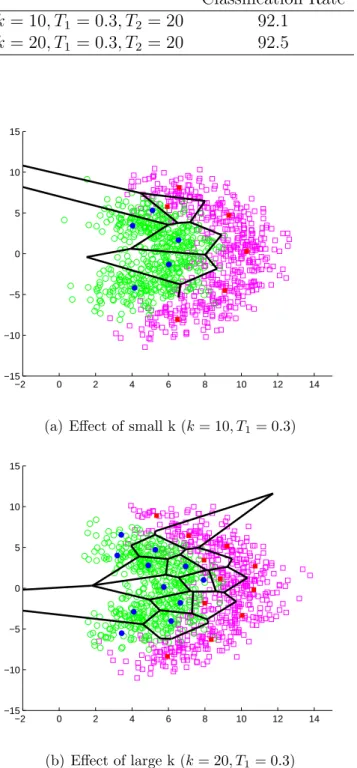
Figure 2.2 demonstrates the effect of increasing the number of initial clusters. As parameter k is increased from 10 to 20, we see that more class centroids are generated in the vicinity of the boundary between two classes. Enabling brute
force searching with single centroid option allows one additional cluster center to be included for k = 20 case while none is included for k = 10 case. The results indicate a slight rise in the classification performance as shown in Table 2.1.
To analyze the effect of increasing T1, we select a high value of initial clusters,
k = 15. So, it is more likely that some class centroids will be discarded for greater
values of T1. This turns out to be a useful choice as depicted in Figure 2.3.
While searching for additional class centroids that better describe the dataset,
T1 = 0.5 case finds a better partitioning of the sample space resulting in a higher
classification accuracy as shown in Table 2.2.
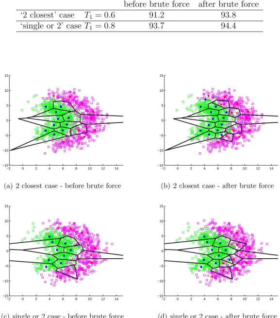
Previously it was mentioned that brute force searching could provide a remedy for accidentally lost class centroids via thresholding. Figure 2.4 demonstrates this idea. By adding only two centroids at each iteration, this example run of the program incorporates 4 additional pairs of cluster centroids that provides a better representation of the data in training set as shown in Table 2.3. ‘2 closest centroids’ and ‘single or 2 centroids’ options listed in the previous section are also investigated in Figure 2.5 and Table 2.4. Combined with a suitable selection of thresholds they also help to construct a better model of the dataset. 3 pairs of closest centroids are added as shown in Figure 2.5(b), and a single and a pair of centroids are added as shown in Figure 2.5(d).
CHAPTER 2. MODIFIED K-MEANS BASED CLASSIFICATION 19
Table 2.1: Effect of increasing k on classification performance Classification Rate k = 10, T1 = 0.3, T2 = 20 92.1 k = 20, T1 = 0.3, T2 = 20 92.5 −2 0 2 4 6 8 10 12 14 −15 −10 −5 0 5 10 15
(a) Effect of small k (k = 10, T1= 0.3)
−2 0 2 4 6 8 10 12 14 −15 −10 −5 0 5 10 15 (b) Effect of large k (k = 20, T1= 0.3)
Figure 2.2: Effect of increasing k on the performance of our modified k-means algorithm. (b) shows that more cluster centers can be obtained in the vicinity of the boundary between two classes.
Table 2.2: Effect of increasing T1 on classification performance
Classification Rate
(after brute force)
k = 15, T1 = 0.3, T2 = 20 92.3 k = 15, T1 = 0.5, T2 = 20 93.8 −2 0 2 4 6 8 10 12 14 −15 −10 −5 0 5 10 15
(a) Before brute force (k = 15, T1= 0.3)
−2 0 2 4 6 8 10 12 14 −15 −10 −5 0 5 10 15
(b) Before brute force (k = 15, T1= 0.5)
−2 0 2 4 6 8 10 12 14 −15 −10 −5 0 5 10 15
(c) After brute force (k = 15, T1= 0.3)
−2 0 2 4 6 8 10 12 14 −15 −10 −5 0 5 10 15
(d) After brute force (k = 15, T1= 0.5)
Figure 2.3: Effect of increasing T1 on the performance of our modified k-means
al-gorithm. Increasing T1 results in ignoring more centroids formed near the
bound-ary at the first stage of our algorithm (b). In some cases this may lead to a better partitioning when brute force searching of the second stage is applied (d).
CHAPTER 2. MODIFIED K-MEANS BASED CLASSIFICATION 21
Table 2.3: Effect of brute force searching on the representation of training set Classification Rate in Training Set
k = 20, T1 = 0.8, T2 = 30
before brute force 92.3
after brute force 93.8
−2 0 2 4 6 8 10 12 14 −15 −10 −5 0 5 10 15
(a) Before brute force searching
−2 0 2 4 6 8 10 12 14 −15 −10 −5 0 5 10 15
(b) After brute force searching
Figure 2.4: Effect of brute force searching on the performance of our modified
k-means algorithm. (b) depicts that a more accurate model can be constructed
with intentionally selecting additional cluster centers that increase classification rate in the training set.
Table 2.4: Effect of other brute force searching methods on the representation of training set
Classification Rate in Training Set
k = 25, T2 = 30
before brute force after brute force
‘2 closest’ case T1 = 0.6 91.2 93.8 ‘single or 2’ case T1 = 0.8 93.7 94.4 −2 0 2 4 6 8 10 12 14 −15 −10 −5 0 5 10 15
(a) 2 closest case - before brute force
−2 0 2 4 6 8 10 12 14 −15 −10 −5 0 5 10 15
(b) 2 closest case - after brute force
−2 0 2 4 6 8 10 12 14 −15 −10 −5 0 5 10 15
(c) single or 2 case - before brute force
−2 0 2 4 6 8 10 12 14 −15 −10 −5 0 5 10 15
(d) single or 2 case - after brute force
Figure 2.5: Effect of different brute force searching methods on the performance of our modified k-means algorithm. In (b), two class centroids which are at minimum distance to each other are selected at every iteration of the brute force approach. In (d), selection is based on picking either one or two (i.e., one from each class) class centroids that increase the success rate most.
CHAPTER 2. MODIFIED K-MEANS BASED CLASSIFICATION 23
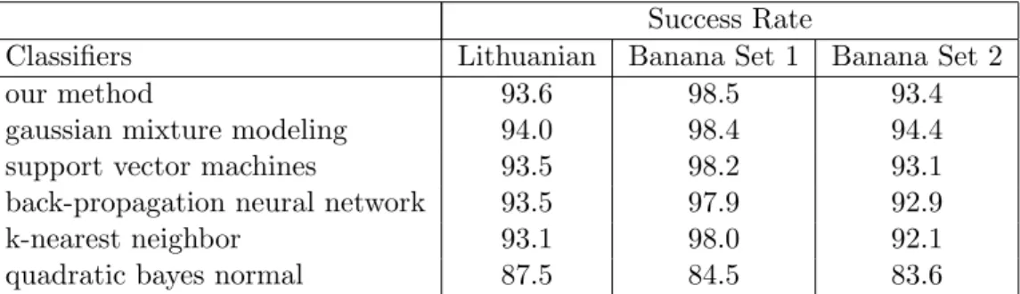
Table 2.5: Performance comparison of our modified k-means algorithm with other well-known classifiers
Success Rate
Classifiers Lithuanian Banana Set 1 Banana Set 2
our method 93.6 98.5 93.4
gaussian mixture modeling 94.0 98.4 94.4
support vector machines 93.5 98.2 93.1
back-propagation neural network 93.5 97.9 92.9
k-nearest neighbor 93.1 98.0 92.1
quadratic bayes normal 87.5 84.5 83.6
2.2.2
Performance Comparison
In this section, we compare the performance of our method with five other state-of-the-art classification algorithms. Two different datasets are provided for per-formance analysis. They are divided randomly into two equal halves: one forming the training set and the other forming the test set.
First one is a dataset of 2000 samples. The data is uniformly distributed along two sausages and is superimposed by a normal distribution with unit standard deviation in all directions. It is a 2-dimensional, 2-class dataset which is usually referred as Lithuanian dataset in the literature. Second dataset is the same size of the first one and contains samples with a banana shaped distribution. The data is uniformly distributed along the bananas and is again superimposed by a normal distribution with unit standard deviation in all directions. A third dataset is generated from the second one by increasing the standard deviation of the superimposed normal distribution to 1.5. Hence, more outliers are generated which will cause higher classification error rates.
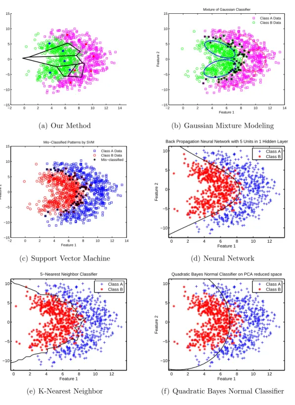
Misclassified sample points, classification boundaries and details of the classi-fiers used are explained for all three datasets in Figures 2.6, 2.7 and 2.8, respec-tively. Success rates are given in Table 2.5. We observe that our classifier out-performs all except gaussian mixture modeling based classifier for two datasets.
In this part, libraries of LIBSVM are used for SVM classification [28]. It en-ables the automatic selection of optimal parameters by employing 10-fold cross validation and an exhaustive search on the parameter space. PRTools is used to optimize parameters, obtain classification errors and draw plots for k-nearest neighbor, back-propagation neural network and quadratic bayes normal classi-fiers [29]. All the code for classiclassi-fiers and plots is written under Matlab 7.0 [30].
CHAPTER 2. MODIFIED K-MEANS BASED CLASSIFICATION 25 −2 0 2 4 6 8 10 12 14 −15 −10 −5 0 5 10 15
(a) Our Method
−2 0 2 4 6 8 10 12 14 −15 −10 −5 0 5 10 15 Feature 1 Feature 2
Mixture of Gaussian Classifier
Class A Data Class B Data
(b) Gaussian Mixture Modeling
−2 0 2 4 6 8 10 12 14 −15 −10 −5 0 5 10 15 Feature 1 Feature 2 Mis−Classified Patterns by SVM Class A Data Class B Data Mis−classified
(c) Support Vector Machine
0 2 4 6 8 10 12 −10 −5 0 5 10 Feature 1 Feature 2
Back Propagation Neural Network with 5 Units in 1 Hidden Layer Class A Class B (d) Neural Network 0 2 4 6 8 10 12 −10 −5 0 5 10 Feature 1 Feature 2
5−Nearest Neighbor Classifier
Class A Class B
(e) K-Nearest Neighbor
0 2 4 6 8 10 12 −10 −5 0 5 10 Feature 1 Feature 2
Quadratic Bayes Normal Classifier on PCA reduced space Class A Class B
(f) Quadratic Bayes Normal Classifier
Figure 2.6: Performance comparison of our modified k-means algorithm with some state-of-the-art classifiers on Lithuanian dataset with 2 classes: (a) Our method (k = 10, T1 = 0.5, T2 = 20), (b) Gaussian Mixture Models using
arbitrary covariance matrices, (c) SVM using radial basis function, (d) Back-propagation Neural Network with 5 units using 1 hidden layer, (e) K-Nearest Neighbors (k = 5), and (f) Quadratic Bayes Normal Classifier on PCA reduced space.
−15 −10 −5 0 5 10 −12 −10 −8 −6 −4 −2 0 2 4 6 8 10
(a) Our method
−12 −10 −8 −6 −4 −2 0 2 4 6 8 −10 −8 −6 −4 −2 0 2 4 6 8 Feature 1 Feature 2
Mixture of Gaussian Classifier
Class A Data Class B Data
(b) Gaussian Mixture Modeling
−12 −10 −8 −6 −4 −2 0 2 4 6 8 −10 −8 −6 −4 −2 0 2 4 6 8 Feature 1 Feature 2 Mis−Classified Patterns by SVM Class A Data Class B Data Mis−classified
(c) Support Vector Machine
−10 −5 0 5 −10 −8 −6 −4 −2 0 2 4 6 Feature 1 Feature 2
Back Propagation Neural Network with 5 Hidden Units in 1 Layer Class A Class B (d) Neural Network −10 −5 0 5 −10 −8 −6 −4 −2 0 2 4 6 Feature 1 Feature 2
5−Nearest Neighbor Classifier
Class A Class B
(e) K-Nearest Neighbor
−10 −5 0 5 −10 −8 −6 −4 −2 0 2 4 6 Feature 1 Feature 2
Quadratic Bayes Normal Classifier on PCA reduced space Class A Class B
(f) Quadratic Bayes Normal Classifier
Figure 2.7: Performance comparison of our modified k-means algorithm with some state-of-the-art classifiers on banana-shaped dataset with 2 classes (randomnessf actor = 1): (a) Our method with minimum distance based brute forcing (k = 25, T1 = 0.6, T2 = 30), (b) Gaussian Mixture Models using
arbitrary covariance matrices, (c) SVM using radial basis function, (d) Back-propagation Neural Network with 5 units using 1 hidden layer, (e) K-Nearest Neighbors (k = 5), and (f) Quadratic Bayes Normal Classifier on PCA reduced space.
CHAPTER 2. MODIFIED K-MEANS BASED CLASSIFICATION 27 −15 −10 −5 0 5 10 −12 −10 −8 −6 −4 −2 0 2 4 6 8 10
(a) Our method
−15 −10 −5 0 5 10 −12 −10 −8 −6 −4 −2 0 2 4 6 8 Feature 1 Feature 2
Mixture of Gaussian Classifier
Class A Data Class B Data
(b) Gaussian Mixture Modeling
−15 −10 −5 0 5 10 −12 −10 −8 −6 −4 −2 0 2 4 6 8 Feature 1 Feature 2 Mis−Classified Patterns by SVM Class A Data Class B Data Mis−classified
(c) Support Vector Machine
−10 −5 0 5 −10 −8 −6 −4 −2 0 2 4 6 8 Feature 1 Feature 2
Back Propagation Neural Network with 5 Hidden Units in 1 Layer Class A Class B (d) Neural Network −10 −5 0 5 −10 −8 −6 −4 −2 0 2 4 6 8 Feature 1 Feature 2
5−Nearest Neighbor Classifier
Class A Class B
(e) K-Nearest Neighbor
−10 −5 0 5 −10 −8 −6 −4 −2 0 2 4 6 8 Feature 1 Feature 2
Quadratic Bayes Normal Classifier on PCA reduced space Class A Class B
(f) Quadratic Bayes Normal Classifier
Figure 2.8: Performance comparison of our modified k-means algorithm with some state-of-the-art classifiers on banana-shaped dataset with 2 classes (randomnessf actor = 1.5): (a) Our method with minimum distance based brute forcing (k = 20, T1 = 0.8, T2 = 30), (b) Gaussian Mixture Models using
arbitrary covariance matrices, (c) SVM using radial basis function, (d) Back-propagation Neural Network with 5 units using 1 hidden layer, (e) K-Nearest Neighbors (k = 5), and (f) Quadratic Bayes Normal Classifier on PCA reduced space.
Image Analysis of Potato Chips
for Acrylamide Formation
This chapter begins with a discussion on how to model acrylamide formation using digital images. It shows that the information contained in CIE a∗ parameter is
not sufficient for this purpose. The chapter continues with an implementation of our algorithm developed in Chapter 2 to estimate acrylamide levels in digital color images of fried potato chips. Normalized-RGB color values are selected as features for the segmentation of acrylamide contaminated areas in digital images. It is experimentally observed that the acrylamide levels in a fried potato chip can be estimated by determining the ratio of brownish yellow regions (obtained via our segmentation algorithm) to the total area of the chip image. We define this ratio as Normalized Area of the Brownish Yellow region (NABY) and linearly correlate it with the acrylamide levels of fried potatoes. The changes of acrylamide levels and NABY values are observed to follow almost the same trend during frying at 170◦C, which indicates a significant correlation between these two variables. We
also demonstrate that autocovariance estimates can be incorporated as additional statistical features into the feature set because they provide a satisfactory level of discrimination.
CHAPTER 3. IMAGE ANALYSIS OF POTATO CHIPS 29
3.1
Modeling Acrylamide Formation using
Im-age Analysis
As explained in the Introduction part, CIE L∗a∗b∗ parameters used to measure
non-homogenous surface color are not reliable predictors of acrylamide concen-tration in potato chips because the acrylamide concenconcen-trations are observed to be lower in darker regions of the potato images. Instead of seeking a linear correla-tion between CIE L∗a∗b∗ parameters and measured acrylamide concentrations, it
may be advantageous to define a specific range of colors for acrylamide estimation. Figure 1.1 shows that potato chips undergo certain color transitions as the frying proceeds. The initial pale soft yellow color of potato first turns to bright yellow, then to brownish yellow during 8 to 10 minutes of frying at 170◦C. After
10 minutes, browning in the surface becomes clearer reaching to a dark brown at the end of frying for 60 minutes. During the frying process, statistical texture and color properties of the digital photo image continuously change and different image regions appear in the given image.
Digital and analog cameras have built-in white-balancing systems modifying actual color values, therefore pixel values in an image captured by a camera of a machine vision system or a consumer camera may not correspond to true colors of imaged objects. In addition, CCD or CMOS imaging sensors of some cameras may not be calibrated during production. Nevertheless, after the frying process, one can clearly visualize three different regions (or equivalently three different kinds of pixels) in a fried potato chip image as shown in Figure 3.1(a): a) bright yellow (Region-1), b) brownish yellow (Region-2), and c) dark brown (Region-3). It is experimentally observed that Region-2 has a high probability of containing acrylamide. This provides us with the possibility of estimating acrylamide levels in a fried potato chip by determining the ratio of brownish yellow regions to the total area of the chip image. An automatic image analysis technique can segment pixels of a fried potato image into three sets and determine their area-wise ratios as shown in Figure 3.1(b). This idea is implemented successfully in the following section using normalized-RGB pixel values.
(a) (b)
Figure 3.1: (a) Original fried potato chip image with selected regions, and (b) Re-sult of our segmentation algorithm described in Section 2.2
3.2
Acrylamide Analysis using CIE a
∗Parame-ter
In this section, we demonstrate our analysis to define a specific range of colors for acrylamide estimation in CIE L∗a∗b∗ color space. In this study, we focus on
CIE a∗ parameter because previous work showed that L∗ and b∗ values did not
show considerable changes as those shown by a∗ during frying of potato chips [6].
3.2.1
Color Spaces
Long before the anatomical discovery of three color receptors (cones) in the human eye, it was proposed that color can be mathematically specified in terms of three variables and different colors can be obtained by mixing them in proper amounts. From then onwards, the idea has been studied extensively under the title of
trichromacy and a number of important concepts have been introduced. Before
CHAPTER 3. IMAGE ANALYSIS OF POTATO CHIPS 31
The sensation of color in human beings can be modeled as the projection of the visible region of electromagnetic spectrum onto the space spanned by three sensitivity functions. The properties of these functions are determined by the response of three types of cones present in the eye. Each cone is either sensi-tive to short, medium or long wavelengths such that the spectral sensitivities of these cones are linearly independent. To capture this sort of behavior, two im-portant concepts are introduced: (a) Color Primaries, and (b) Color Matching Functions (CMF).
Color primaries are three colorimetrically independent light sources where each source is a collection of the visible electromagnetic spectra. Independence guarantees that the color of any primary cannot be visually matched by a linear combination of the remaining two primaries. These primaries are used to obtain a nonsingular linear transformation of the sensitivities of the three cones in the eye, defined as a CMF [31]. This, in turn, allows us to the represent the color of a visible spectrum in terms of tristimulus values (obtained via a color match-ing transformation) instead of actual cone sensitivity values. In order to prevent any confusion, it is necessary to specify with respect to which CMF the tris-timulus values are computed. CIE, International Commission on Illumination, developed a number of standards to serve this purpose.
After careful studies on human color perception, two equivalent sets of CMFs are first defined by the CIE in 1931: (1) CIE Red-Green-Blue (RGB), and (2) CIE
XYZ. They are based on direct measurements of the human eye. The three
monochromatic primaries used in the first set are at wavelengths of 700 nm (red), 546.1 nm (green) and 435.8 nm (blue). The second set of CMFs is obtained by a linear transformation of the CIE RGB CMFs and the following relation exists between the tristimulus values in CIE XYZ and CIE RGB spaces.
X Y Z = 0.488718 0.310680 0.200602 0.176204 0.812985 0.0108109 0.000000 0.0102048 0.989795 r g b
range [0.0, 1.0]. The output values are also in the unit range.
CIE xy chromaticity space is derived from X,Y,Z tristimulus values in the CIE
XYZ space according to the equations below:
x = X X+Y +Z y = Y X+Y +Z z = Z X+Y +Z
3.2.2
Color Differences and CIE L
∗a
∗b
∗Color Space
Perceptual uniformity is an important property for a variety of industrial ap-plications. It requires that equal perceived color differences should correspond to equal Euclidean distances in the tristimulus color space. However, the color spaces we mentioned so far are perceptually nonuniform. For this reason, spe-cial emphasis was given to develop a device-independent, perceptually uniform representation of all the colors visible to the human eye. The concept of Just
No-ticeable Difference (JND) was introduced to quantify small color changes and a
distance metric based on MacAdam ellipse was used. MacAdam ellipse defines a region on a chromaticity diagram such that all colors which are indistinguishable to the average human eye from the color at the center of the ellipse are grouped together.
In an attempt to linearize the perceptibility of color differences, CIE recom-mended L∗a∗b∗ color space in 1976. In L∗a∗b∗ space, L∗ represents the luminance
of the color and ranges in the interval [0, 100], 0 indicating black and 100 indicat-ing white. As a∗ changes from negative values to positive values, the position of
the color moves from green to red. Similarly, b represents the position of the color between blue and yellow, negative values yielding blue and positive values yield-ing yellow. A reference illumination parameter, called whitepoint is also used to provide a crude approximation for eye’s adaptation to white color under different lighting conditions.
CHAPTER 3. IMAGE ANALYSIS OF POTATO CHIPS 33
3.2.3
Conversion from CIE XYZ to CIE L
∗a
∗b
∗CIE L∗a∗b∗ space is defined with the following nonlinear transformation from CIE XYZ tristimulus color space:
L∗ = 116f³Y Yn ´ − 16 a∗ = 500³f³X Xn ´ − f ³ Y Yn ´´ b∗ = 200³f³Y Yn ´ − f ³ Z Zn ´´ where f (x) = ( x1/3 x > 0.008856 7.787x + 16 116 x ≤ 0.008856
and Xn, Yn, Znare the tristimuli of the white stimulus. Under this transformation,
a JND corresponds to an Euclidean distance of 2.3.
3.2.4
Practical Issues
An RGB image is described with red, green and blue pixel values but these values are not standardized and do not have precise definitions. RGB is not an absolute, device-independent color space like CIE XY Z or L∗a∗b∗, and a direct conversion
formulae between RGB and L∗a∗b∗ spaces have no meaning. Therefore, an RGB
image may look considerably different from one monitor to another.
To overcome this effect, a standard has been adopted recently by major manu-facturers to characterize the behavior of an average CRT monitor.1 All non-CRT
hardware, such as LCD screens, digital cameras and printers are also built with additional circuitry or software to obey this standard. For this reason, it is in general safe to assume that an image file with 8 bits per channel is in sRGB space and a meaningful conversion can be defined between sRGB and L∗a∗b∗ spaces. sRGB values are first transformed into CIE XY Z space as follows:
X Y Z = 0.412424 0.357579 0.180464 0.212656 0.715158 0.0721856 0.0193324 0.119193 0.950444 r g b where r = ( R/12.92 R ≤ 0.04045 ((R + 0.055)/1.055)2.4 R > 0.04045 g = ( G/12.92 G ≤ 0.04045 ((G + 0.055)/1.055)2.4 G > 0.04045 r = ( B/12.92 B ≤ 0.04045 ((B + 0.055)/1.055)2.4 B > 0.04045
Input RGB values are scaled to unit range. Output XYZ values are also in unit range [0.0, 1.0]. CIE XY Z values are then nonlinearly mapped into CIE
L∗a∗b∗ space using the same method discussed above. D65 daylight illumination
is used as reference white in these calculations. A more rigorous discussion about conversion operations can be found in the following references [32, 33, 34].
3.2.5
Results and Discussion
Gokmen et al. measured CIE a∗values for potato chips shown in Figure 3.2 using a
Minolta CM-3600d model spectrophotometer. Potato chips were fried at 170◦C
with sampling at 1, 3, 5, 8, 10, 15, 30 and 60 minutes. The results are shown in
Figure 3.2: Potato chip images used for acrylamide analysis aligned according to frying time
CHAPTER 3. IMAGE ANALYSIS OF POTATO CHIPS 35
Table 3.1: Measured acrylamide concentration, measured and estimated CIE a∗
values for potato chips
t, min AA, ng/g Measured CIE a∗ Estimated CIE a∗
1 582 1.96 5.013 3 2554 5.35 8.6375 5 9519 11.73 20.6559 8 10963 12.47 22.6269 10 10500 12.78 23.0435 15 8198 12.92 27.7742 30 5119 13.86 30.6953 60 4987 13.55 30.9508
Table 3.1. From these results, it is not possible to define a specific range of CIE
a∗ values for acrylamide estimation because a∗ values are very close to each other
for brownish yellow and dark brown colored potatoes.
We estimate average CIE a∗ values from RGB images of fried potato chips
following the formulation described in the previous sections. Using Matlab 7.0 built-in functions for color conversions (makecform,applycform), potato chip im-ages (See Figure 3.2) are transformed from RGB into CIE L∗a∗b∗ color space. An
average CIE a∗ value is calculated for each potato chip image by taking the mean
of all extracted a∗ values. As shown in Figure 3.3 and Table 3.1, high acrylamide
concentrations are observed for intermediate values of a∗ parameter. Lower
val-ues of a∗ indicate a decrease in measured acrylamide concentration. However,
higher values of a∗ do not indicate such a clear decrease and defining a specific
range responsible for acrylamide formation from estimated CIE a∗ values is not
possible, either. Hence, we turn our attention to a new set of features explained in the following section.
Figure 3.3: Change of acrylamide concentration and estimated CIE redness pa-rameter a∗ in potato chips during frying at 170◦C
3.3
K-means Clustering based Segmentation for
Acrylamide Analysis in Potato Chip Images
As mentioned in Chapter 3.1, the segmentation of fried potato images into three regions can provide us the necessary information to estimate acrylamide levels. Several state-of-the-art image segmentation and pattern classification algorithms are available in the literature each having its own advantages and disadvantages. For a complete discussion of these algorithms, the reader may refer to any of the following references [35, 36, 37, 19, 38].
In this section, we analyze digital color images of fried potatoes to estimate acrylamide levels using the method developed in the previous chapter. We show that acrylamide levels in a fried potato image can be estimated by determining the ratio of brownish yellow regions to the total area of a given potato chip, abbreviated as NABY. Three different regions corresponding to bright yellow,
CHAPTER 3. IMAGE ANALYSIS OF POTATO CHIPS 37
brownish yellow and dark brown are extracted using our k-means based classi-fier and their corresponding area-wise ratio is calculated using the segmentation results obtained from the classifier.
3.3.1
Selected Features
A typical image captured by a digital camera consists of an array of vectors called pixels. Each pixel x[n, m] has red, green and blue color values:
x[n, m] = xr(n, m) xg(n, m) xb(n, m)
where xr(n, m), xg(n, m) and xb(n, m) are the values of red, green and blue
com-ponents of the (n, m)thpixel x[n, m], respectively. In digital images, x
r, xg and xb
color components are represented in 8 bits, i.e., they are allowed to take integer values between 0 and 255(= 28−1) [37]. Digital and analog cameras have built-in
white balancing systems modifying actual color values, therefore pixel values in an image captured by a camera of a machine vision system or a consumer camera may not correspond to true colors of imaged objects. In addition, CCD or CMOS imaging sensors of some cameras may not be calibrated during production. To reduce such variations due to lighting conditions and white-balancing scheme of digital cameras, normalized image pixel color values are used as features for our classification system.
Figure 3.5 plots the distribution of the normalized color values obtained from the regions shown in Figure 3.4. From this figure, we deduce that a set of features containing only normalized color values can be enough to provide a reasonable separation of the dataset using our k-means based classifier. They are computed as follows:
xr(n, m) = xr(n, m) xr(n, m) + xg(n, m) + xb(n, m) xg(n, m) = xg(n, m) xr(n, m) + xg(n, m) + xb(n, m) xb(n, m) = xb(n, m) xr(n, m) + xg(n, m) + xb(n, m)
(a) Bright Yellow (b) Brownish Yellow (c) Dark Brown
Figure 3.4: Potato regions used in feature distribution and autocovariance esti-mation plots (a) Region 1, (b) Region 2, and (c) Region 3
0.2 0.4 0.6 0.8 1 0 0.2 0.4 0.6 0.8 0 0.1 0.2 0.3 0.4 Region I Region II Region III
Figure 3.5: Distribution of the features used for acrylamide level estimation in normalized RGB space.