arXiv:1205.2288v1 [astro-ph.IM] 10 May 2012
A Dynamic Era-Based Time-Symmetric Block
Time-Step Algorithm with Parallel Implementations
Murat KAPLAN
Akdeniz University, Space Sciences and Technologies, TR-07058 Antalya,Turkey [email protected]
Hasan SAYGIN
˙Istanbul Aydın University, Be¸syol Mah. In¨on¨u Cad. No:38 Sefak¨oy-K¨u¸c¨uk¸cekmece,˙Istanbul, Turkey [email protected]
(Received ; accepted )
Abstract
The time-symmetric block time–step (TSBTS) algorithm is a newly developed efficient scheme for N–body integrations. It is constructed on an era-based iteration. In this work, we re-designed the TSBTS integration scheme with dynamically chang-ing era size. A number of numerical tests were performed to show the importance of choosing the size of the era, especially for long time integrations. Our second aim was to show that the TSBTS scheme is as suitable as previously known schemes for developing parallel N–body codes. In this work, we relied on a parallel scheme us-ing the copy algorithm for the time-symmetric scheme. We implemented a hybrid of data and task parallelization for force calculation to handle load balancing prob-lems that can appear in practice. Using the Plummer model initial conditions for different numbers of particles, we obtained the expected efficiency and speedup for a small number of particles. Although parallelization of the direct N–body codes is negatively affected by the communication/calculation ratios, we obtained good load balance results. Moreover, we were able to conserve the advantages of the algorithm (e.g., energy conservation for long–term simulations).
Key words:N–body: parallel algorithms: celestial mechanics: stellar dynamics
1. Introduction
In many practical applications in N–body integrations, the block time–step approach is preferred. In this approach, many particles share the same step size, where the only allowed values for the time–step length are powers of two. Block time–steps are advantageous to reduce the prediction overheads, and are needed both for good parallelization and code efficiency.
However, the time-symmetricity and symplecticity of previous direct integration schemes are disturbed by using variable block time–steps.
The algorithm developed by Makino et al (2006) (TSBTS) is the first algorithm for time symmetrizing block time–steps which carry the benefits of time symmetry to block time–step algorithms. In this algorithmic approach, the total history of the simulation is divided into a number of smaller periods, with each of these smaller periods called an “era”. Symmetrization is achieved by applying a time symmetrization procedure with an era-based iteration.
The TSBTS algorithm was generated for direct integration of N–body systems and as such is suitable to use for a moderate number of bodies no more than 105
. The direct approach to N–body integration is preferred when we are interested in the close-range dynamics of the particles, and aiming at obtaining high accuracy. The algorithm gives us the ability to reach long integration times with high accuracy. However it has some limitations on memory usage which stem from choosing the size of the era.
The TSBTS algorithm also provides some benefits for parallelization of N–body al-gorithms. Development of parallel versions of variable time–step codes becomes increasingly necessary for many areas of research, such as stellar dynamics in astrophysics, plasma simula-tions in physics, and molecular dynamics in chemistry and biology. The most natural way to do this is through the use of block time–steps, where each particle has to choose its own power of two, for the size of its time–step (Aarseth 2003). Block time–steps allow efficient parallelization, given that large numbers of particles sharing the same block time–step can then be integrated in parallel.
In Section 2, we summarize the TSBTS algorithm time-symmetric block time–step al-gorithm. We provide definitions for the era concept, and for time-symmetrization of block time–steps. In Section 3, we present sample numerical tests for choosing the size of the era. We show how important is the effect of the era size on the energy errors, and the relationship between era size and iteration number. In Section 4, we offer a dynamic era size scheme for both better energy conservation and better memory usage. In Section 5, we present a parallel algorithm for the TSBTS scheme with a hybrid force calculation procedure. In Section 6, we discuss load balance and parallel performance tests of the algorithm. Section 7 sums up the study.
2. Era-Based Iterative Time Symmetrization for Block Time Steps
In the TSBTS algorithm, an iterative scheme is combined with an individual block time–step scheme to apply the algorithm to the N–body problem effectively. There are two important points in this algorithm: the era concept and the time-symmetrization procedure. The era is a time period in which we collect and store information for all positions and velocities of the particles for every step. At the end of each era, we synchronize all particles with time symmetric interpolation. This synchronization is repeated many times during the integration
period, depending on the size of the era.
Let us remember the TSBTS algorithm briefly: We used a self-starting form of the leapfrog scheme;
rnew= rold+ vold∆t +
1 2aold∆t 2 , vnew= vold+ 1 2(aold+ anew)∆t, (1)
with Taylor expansion for predicted velocities and positions;
rpnew= rold+ vold∆t +
1 2aold∆t
2
,
vnewp = vold+ aold∆t. (2)
One of the easiest estimates for the time–step criterion is the collisional time–step. When two particles approach each other, or move away from each other, the ratio between relative distance and relative velocity gives us an estimation.
On the other hand, if particles move at roughly the same velocity, the collision time scale estimate produces infinity when the particles’ relative velocities are zero. For such cases, we use a free fall time scale as an additional criterion, or just take the allowed largest time–steps for those particles.
Time-steps are determined using both the free-fall time scale and the collision time scale (3) for particle i by taking the minimum over the two criterion and over the all j as;
δti= η min i6=j |rij| |vij| , v u u t |rij| |aij| (3)
where η is a constant accuracy parameter, rij and vij are the relative position and velocity
between particles i and j, and aij is the pairwise acceleration.
Even if Aarseth’s time–step criterion (Aarseth 2003) serves us better in avoiding such unexpected situations and gives us a better estimation, it needs higher order derivatives and it is expensive for a second order integration scheme.
Our time-symmetry criterion is defined in Eq.4. This criterion gives us the smallest n values that suit the condition ∆tn≤ δtmi ;
n = min k≥1 ( k 1 2k−1 ≤ (δtm i + δt m+1 i ) 2 ) (4)
where m is the iteration counter. Here, m and m + 1 refer to the beginning and end of the time step.
In the case of block time–step schemes, a group of particles advances at the same time. At each step of the integration, a group of particles is integrated with the smallest value of ∆tn. Here, we refer to the group of particles as particle blocks. The first group of particles in
In the first pass through an era, we perform standard forward integration with the standard block step scheme, without any intention to make the scheme time–symmetric. To compute the forces on the particles with the smallest value of ∆tn, we use second-order Taylor
expansions for the predicted positions, while a first-order expansion suffices for the predicted velocity. Predicted positions, velocities, and accelerations for each particle for every time–step are stored during each era.
In the second pass, which is the first iteration, instead of Taylor expansions we use time-symmetric interpolations with stored data. This time, each time–step is calculated in a different way for symmetrization as in Algorithm 1. Here, dtm is the block time–step of the
integrated particle group, and ∆tn is the n’th level block time–step, which is obtained from a
time-symmetry criterion (Eq.4). If the current time is an even multiple of the current block time–step, that time value is referred to as even time, otherwise it is referred to as odd time.
Algorithm 1: Symmetrization Scheme for Block Time Steps for m = 1 to number of iteration do
if time == odd time then if dtm6= ∆tn then
dtm= dtm/2
end if end if
if time == even time then if dtm< ∆tn then dtm= dtm∗ 2 end if if dtm== ∆tn then dtm= ∆tn end if if dtm> ∆tn then dtm= dtm/2 end if end if end for
Here is the description of the symmetrization scheme for block time–steps (as in Algorithm 1):
If the current time is odd, first, we try to continue with the same time–step. If, upon iteration, that time–step qualifies according to the time-symmetry criterion (as in Eq.4), then we continue to use the same step size that was used in the previous step of the
iteration. If not, we use a step size half as large as that of the previous time–step.
If the current time is even, our choices are: doubling the previous time–step size; keeping it the same; or halving it. We first try the largest value, given by doubling. If Eq.4 shows us that this larger time–step is not too large, we accept it: otherwise, we consider keeping the time–step size the same. If Eq.4 shows us that keeping the time–step size the same is okay, we accept that choice: otherwise, we simply halve the time–step, in which case no further testing is needed.
The same steps are repeated for higher iterations as in the first iteration. The main steps of the integration cycle is given by Algorithm 2.
Algorithm 2: Sequential Algorithm for TSBTS
1: Initialization:
- Read initial position and velocity vectors from the source. - Arrange size in the memory.
- Initialize particles’ forces, time–steps, and next block times. - Sort particles according to time blocks.
2: Start the iteration for the era.
3: Start the integration for the first block of the era.
4: Predict position and velocity vectors of all particles for the current integration time. If this is the first step of the iteration, or if the time of the particle is smaller than the current time, do direct prediction: otherwise perform interpolation from the currently stored data.
5: Calculate forces on the active particles.
6: Correct position and velocity vectors of the particles in the block.
7: Update their new time–steps and next block time.
- After the first iteration, symmetrize new time steps according to Algorithm 1.
8: Sort particles according to time blocks.
9: Repeat from Step 3 while current time is ≤ time at the end of the era.
10: Repeat from Step 2 until the number of the iteration reaches the iteration limit.
11: Repeat from Step 2 for the next era, until the final time is reached. 12: Write the outputs and finish the program.
3. Numerical Tests for the Size of the Era
The size of an era can be chosen as any integer multiple of the maximum allowed time– step. There is not any important computational difference between dividing the integration to the small era parts and taking the whole simulation in one big era. However some sym-metrization routines such as adjusting the time–steps and interpolating the old data increase the computation time. Additionally, keeping the whole history of the simulation requires a
huge amount of memory.
It is important to decide what is the most convenient choice for an era. We need to store sufficient information from the previous steps to adjust the time–steps with iterations. To avoid doing additional work and storing a uselessly large history, choosing a large size for the era is not recommended. On the other hand, the era size must be large enough to store rapid and sharp time–step changes.
We made several tests with different Plummer model initial conditions, using different sizes of era. Units were chosen as standard N–body units (Heggie and Hut 2003), as the gravitational constant G = 1, the total mass M = 1 and the total energy is Etot = −1/4. We
limited the maximum time–step to 1/64. The η parameter was kept larger than usual to see the error growth in smaller time periods. The η parameter was set as 0.1 for 100-body problems, and 0.5 for 500-body problems. The Plummer type softening length ǫ was taken as 0.01. Each system was integrated for every era size (1, 0.5, 0.25, 0.125, 0.0625, 0.03125, 0.015625) for 1000 time units.
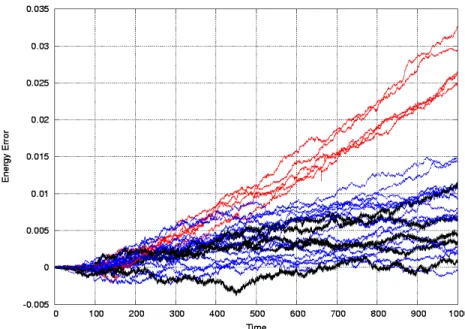
Fig.1 shows the energy errors for 5 different 100-body problems with 5 different era sizes. In these test runs, time-symmetrized block time–steps were used with 3 iterations. We also performed test runs for other era sizes (1.0,0.5). However, the growth of energy errors for these era sizes reached beyond the scales of this figure. The figure shows that, 3 iterations are not enough to avoid linearly growing errors for large (here, 0.25) era sizes.
We conducted the following tests to see this effect clearly. Fig.2 shows the energy errors for 5 different 100-body problems with 5 different era sizes as in the previous figure. However, we used 5 iterations here. In this figure, the largest era size (0.25 time unit) does not show a linearly growing error exactly the contrary to the case of 3 iterations.The improvement on energy errors comes directly from the iteration process as we expected.
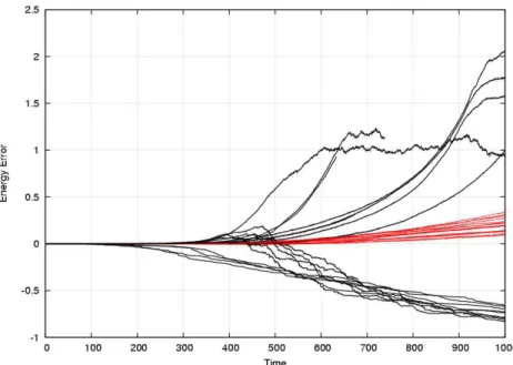
We increased the particle number 5 times, and set the η parameter as 0.5. The η parameter could have been kept as 0.1, but we forced the algorithm to take larger time–steps, which in turn produce larger energy errors for relatively small time periods. Fig.3 shows the energy errors for 5 different 500-body problems with 7 different era sizes. The red curves show the errors for era sizes of 0.015625, 0.03125, and 0.0625 time units; the black curves show the errors for era sizes of 0.125, 0.25, 0.5, and 1 time units.
It seems that more iterations are needed to obtain smaller energy errors while working with larger era sizes. If time-symmetric block time–steps can not be produced with a small number of iterations, the total energy error grows linearly. As indicated by our tests, iteration number and era size must be chosen carefully to ensure symmetric block time–steps.
Although the size of the era is not very important as long as the iteration number is large enough, a high number of iterations is not the preferred choice, as it demands high computational cost. Also, the era size would have to be kept small to avoid the huge memory usage. In practice, our tests show that, 5 iterations is not enough to prevent linearly growing
Fig. 1: Relative energy errors for 100-body problems. 5 different sets of Plummer model initial conditions with 5 different era sizes (0.015625, 0.03125, 0.0625,0.125,0.25) are used with 3 iterations for 1000 time units. The top 5 curves (red curves) show linearly growing errors that correspond to errors for the largest era sizes (0.25). The rest of the curves present the results for other era sizes. The smallest relative errors in the figure (black curves) show a random-walk fashion and correspond to results to the smallest era size (0.015625).
errors when we use greater than 0.25 time unit as the era size.
On the other hand, the era size must be greater than the greatest time–step. Otherwise we can not store past information for the iteration process and the algorithm works as a classical block time–step scheme.
4. Dynamic Era
Our test results for symmetrized time–steps with a small number of iterations in the previous section show that keeping the era size large or small has a clear effect on energy errors. However, the amount of the past position and the velocity information increase with the size of the era. Then, many more iterations are required to obtain optimized time–steps. And increased numbers of iterations consume more CPU time.
Let us remember and give some additional details and definitions about the relationship between block time–steps and era: similar to the first block definition we provided in Section 2, the last group of particles in an era is referred to as the last block. The current time in the integration for the first and last blocks are referred to as first block time and last block time,
Fig. 2: Relative energy errors for 100-body problems. 5 different sets of Plummer model initial conditions are used for 5 iterations with 5 different era sizes (0.015625, 0.03125, 0.0625,0.125,0.25). In this figure, all of the curves show random-walk fashion instead of linearly growing errors. Also, the worst relative error is below 0.008 even when it is 0.035 in Fig.1.
respectively.
At the end of each era, integration of every particle stops at the same time, and new block time–steps are calculated and assigned for new blocks. The last block can take the maximum allowed time–step at the most. The first block can take any block time–step smaller than the maximum allowed time–step. Then, particles are sorted according to their block time–steps. Also, every block has its own integration time related to its block time–step.
If we can find the proper criterion to change it, era size can be controlled dynamically. The simplest choices can vary between 1 time unit and the allowed largest time–step. Our suggestion is: calculate the new block time–steps and the first and last block times at the end of each era, and take the difference between the last and first block times. This difference gives us a dynamically changing size and we can assign this as the size of the new era.
Naturally, sometimes this difference can be larger than 1 time unit, or smaller than the maximum allowed time–step. Also, if all of the particles take the same time–step in any era, the difference goes to zero. We can use the maximum allowed time–step and any power-of-two times of this era size for the top and bottom limits of the era, respectively. Here, we used 2−3 multiples of the largest time–step for the lower limit. If all of the particles take the
largest time–step, or larger time–steps than the new era size, there will not be enough past information for symmetrization. For these reasons, era size must not be much smaller than the
Fig. 3: Relative energy errors for 500-body problems. 5 different sets of Plummer model initial conditions are used with 7 different era sizes (0.015625, 0.03125, 0.0625, 0.125, 0.25, 0.5, 1) for each set. 3 iterations are performed in the integrations. 15 curves (red curves) in the center of the figure present the results of smaller era sizes (0.015625, 0.03125, 0.0625); the rest of the 20 curves correspond to larger (0.125, 0.25, 0.5, 1) era sizes.
largest time–step.
If our estimate of the era size is smaller than our largest time–step, the particles with largest time–steps are excluded from the integration process of the era, and are then left for the next era. Errors of energy conservation oscillate in time, when they happen. We can use the allowed largest time–step for the era size in these cases. The main steps of the algorithm is given by Algorithm 3.
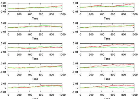
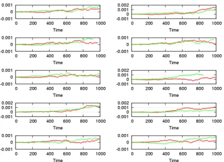
In the tests we did for the dynamic era, we used two choices for era size: equal to the allowed largest time–step, and dynamically changing size as defined above. We already know from previous runs for these test problems that we obtained the smallest errors on total energies when we took the allowed largest time–steps as the era size. We performed 3 iterations. Fig.5 shows the energy errors for 10 different 500-body problems. The green curves show the results for the dynamically changing era; the red curves show the results for the fixed era. Fig.4 shows the energy errors for 10 different 100-body problems.
The results for dynamic era size are in the same range with those of fixed era size. Even if the chosen fixed era size (0.015625) seems like the best choice for previous tests with the same initial conditions and parameters (i.e., maximum allowed time–steps, softening and accuracy parameters), in general, dynamic era gives modestly better results than fixed era for 0.015625.
Algorithm 3: Sequential Algorithm for TSBTS with Dynamic Era Size
1: Initialization (same as Algorithm 2).
2: Set first and last block times.
3: Calculate dynamic era size (dynamic era size = last block time - first block time i) if dynamic era size < 2 ∗ 10−3∗ maximum time step
dynamic era size = 2 ∗ 10−3∗ maximum time step
ii) if dynamic era size > maximum time step dynamic era size = maximum time step
4: Start the iteration for the era.
5: Start the integration for the first block of the era.
6: Predict position and velocity vectors of all particles for the current integration time. If this is the first step of the iteration, or if the time of the particle is smaller than the current time, do direct prediction: otherwise perform interpolation from the currently stored data.
7: Calculate forces on the active particles.
8: Correct position and velocity vectors of the particles in the block.
9: Update their new time–steps and next block time.
- After the first iteration, symmetrize new time steps according to Algorithm 1.
10: Sort particles according to time blocks.
11: Repeat from Step 5 while current time is ≤ time at the end of the era.
12: Repeat from Step 4 until the number of the iteration reaches the iteration limit.
13: Repeat from Step 2 for the next era, until the final time is reached. 14: Write the outputs and finish the program.
We ran more than 20 tests, and in 45% of them were the errors for dynamic era size larger than errors for fixed era size. The rest of the results are clearly better than those for fixed era sizes, besides the advantage of reduced memory usage for the same number of iterations. Running times for dynamic era size are 10% less than for fixed era sizes in general.
5. Parallel Algorithm
Basically, there are two well known schemes that are used in direct N–body paralleliza-tions: copy and ring.
The ring algorithm is generally preferred for reducing memory usage. It can be reason-able for shared time–step codes, but it is not easy to use with block step schemes. It is also well known from previous works that this algorithm achieves almost the same speedup as the copy algorithm (Makino 2002). The number of the particles in the integrated block changes with every step. In many cases, the size of the integrated block can be smaller than the number of the processors. It is difficult to obtain balanced load distribution for such cases.
Fig. 4: Relative energy errors for 10 different 100-body problems. For each initial condition, two algorithms are performed, one with fixed and one with changing era size. 3 iterations are used for two algorithms. Fixed era size was taken as 0.015625. This value was also used as the allowed largest time–step for the algorithms. The green curves correspond to dynamic era sizes and 70% of them show smaller errors than fixed sizes.
the copy algorithm also has the load imbalance problem in classical usage. For any case, block size can be smaller than the number of processors again.
We divided the partitioning strategy into two cases to avoid bad load balancing. In the first case, we divided the particles when the number of particles in the first block is greater than number of nodes. This is a kind of data partitioning, with every node containing a full copy of the system. In the second case, we divide the force calculation of the particles in the first block as a kind of work partitioning.
Our parallel algorithm works with the following steps, as in Algorithm 4.
6. Load Balance and Performance
We have performed test runs on a Linux cluster in ITU-HPC Lab.1
with 37 dual core 3.40 GHz Intel(R) Xeon(TM) CPU with Myrinet interconnect.
The compute time was measured using MPI Wtime(). The timing for total compute time was started before the broadcast of the system to the nodes, and ended at the end of integration. The calculation time of the subset of the particles in the current time block that
Fig. 5: Relative energy errors for 10 different 500-body problems. Fixed and dynamic era sizes are performed for each initial condition, as in Fig.4. Fixed era size and allowed largest time– step were taken as 0.015625 just as in previous tests. The results for dynamic and fixed era sizes are in the same error ranges (40% of them show smaller errors than fixed sizes), and no linearly growing error is observed.
are being handled by a given processor was taken as the work load of the processor. In the iteration process, the largest time was taken as the work load of the processor for the same time block.
Work load of the i’th processor for every active integrated particle group is defined as wi; np is the number of processors; the mean work load hW i is:
hW i = 1 np np X i=1 wi, (5)
and load imbalances:
L(w) = 1 − hW i max(wi)
. (6)
Fig.6 shows the load imbalance for a 1000-body problem. We used 12 processors. In direct N–body simulations, a 1000 body is not a big number for 12 processors (Makino 2002; Harfst et al 2007; P. Spinnato 2000). Here, load imbalance is not seen as more than 0.1% in general. Moreover, load imbalance is smaller than expected. The main reason for this is in the iteration routines of the TSBTS algorithm, which increases both communication and calculation times for active particles. Also, when the number of particles in the first block is smaller than the number of nodes, work partitioning is applied in the algorithm, which also
Algorithm 4: Parallel TSBTS Algorithm
1: Broadcast all particles. Each node has a full copy of the system.
2: Initialize the system for all particles in all nodes. Every node computes time–steps for all
particles.
3: Compute and sort time blocks.
4: Integrate particles in the first block whose block times are the minimum for the era: i) if the number of the first block ≥ number of nodes: every processor
calculates forces and integrates
(number of first time block)/(number of nodes) particles.
ii) if the number of the first block < number of nodes: every processor calculates (number of particles)/(number of nodes) part of the forces on the particles of the first block.
5: Update integrated particles.
6: Repeat from Step 3.
increases communication time.
T1is the running time for one processor; Tnis the running time for n processors. speedup,
and efficiency are given respectively, as:
speedup= T1 Tn , (7) efficiency= T1 n ∗ Tn . (8)
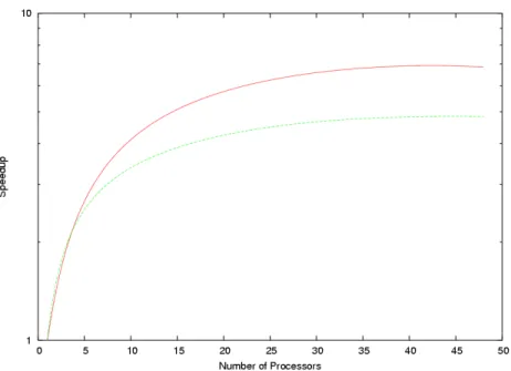
Fig.7 and Fig.8 show speedup and ef f iciency results of symmetrized and non-symmetrized block time–steps for an 10000-body problem initial conditions with Plummer softening length of 0.01 and accuracy parameter η = 0.1. Only one iteration with the TSBTS algorithm corresponds to individual block time–step algorithm without symmetrization. The speedup result for 3 iterations is clearly better than the result for 1 iteration. These results show that the communication/calculation ratio decreases with the iteration process, though iteration needs much more computation time.
For moderately short integration times, as in one time unit cases, the same error bounds can be obtained with less computation times by classical algorithms. However, the algorithm already shows its advantages in long time integrations. Fig.9 shows relative energy errors and CPU times for 20 different 500-body problems with 2 different accuracy parameters (η = (0.1, 0.01)) for 1 CPU. Each system was integrated for 1 and 3 iterations and 1000 time units. Even if it is not possible to obtain the same degree of energy errors for different test problems, the results are still highly promising. We obtained significantly better energy errors with the TSBTS algorithm (3 iterations) than with the classical individual block time–step algorithm (1 iteration) for the same accuracy parameters (η = 0.1) in all tests. Also, in some tests (more
Fig. 6: Load imbalance for 1000-body problem Plummer model initial conditions using 12 processors for 1000 time units. η = 0.1; era size is taken as the allowed largest time–step. Every single red point corresponds to a load imbalance for the active particle group at the time when its vectors are updating.
or less in 20% of the tests), we obtained better results with 3 iterations for 10 times larger accuracy parameters than with 1 iteration runs for η = 0.01.
For example in one of our 500-body problems, we obtained a relative energy error of 5.4 ∗ 10−5 with η = 0.1 for 3 iterations, while it was 3.1 ∗ 10−2 for 1 iteration. To reach the same
error bound with one iteration for 1000 time units, we had to reduce the accuracy parameter to 10 times smaller (η = 0.01). Then, we obtained relative energy error of 1.92 ∗ 10−5 with 1
iteration. In this example, calculation times for 1 and 3 iterations with η = 0.1 were 6.77 ∗ 103
sec., and 3.28 ∗ 104
sec. respectively, while the time was 6.36 ∗ 104
sec. for η = 0.01 with 1 iteration. Here, 3 iterations increase the calculation time by almost a multiple of 2. However, calculation time increases by a multiple of 10, while the accuracy parameter is reduced by the same order.
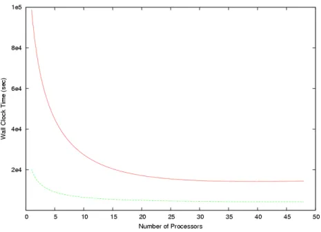
Fig.10 shows running time requirements of the algorithm for the same 10000-body prob-lem, both for 1 and 3 iterations, for one N–body time unit. The TSBTS algorithm needs up to 5 times more run time than 1 iteration case with 1 CPU for this test (for 500-body tests, this ratio was 4.75 as an average of their run times). This extra time is consumed by iteration and symmetrization procedures. The time-consuming ratio between the 1 and 3 iteration cases reduces to almost 3.5 times when we increased the number of processors.
Fig. 7: Speedup vs. processor number for 10000-body problem Plummer model initial condi-tions, both for symmetrized and non-symmetrized individual block time–step algorithms. The continuous curve at the top corresponds to symmetrized block time–steps with 3 iterations. The discontinuous curve at the bottom corresponds to the classical block time–step algorithm.
7. Discussion
We have analyzed the era concept in greater detail for time symmetrized block time– steps. Our test results show that the size of the era must be chosen carefully. This is important, especially for long-term simulations with highly desirable energy conservations. The era size is also important to avoid the need for additional data storage and a uselessly high number of iterations, which require too much running time.
In this work, we suggested a dynamically changing size for the era. This enables us to follow the adaptively changing size for these time periods. In this scheme, the era size will be well-adjusted to the physics of the problem. In many cases, we obtained better energy errors than previous algorithm with fixed era size.
Additionally, we produced a copy algorithm-based parallel scheme combining with our time symmetrized block time–step scheme. We divided the force calculation into two ap-proaches, according to the number of the integrating particles, to avoid bad load balancing. If the number of particles in the integrated block was greater than the number of processors, we used the classical approach –the copy algorithm– to calculate forces. If we had a lower number of particles than processors to integrate, we divided the force calculations between the processors using work partitioning.
Fig. 8: Efficiency vs. processor number for 10000-body problem Plummer model initial condi-tions, both for symmetrized and non-symmetrized individual block time–step algorithms. The continuous curve at the top corresponds to symmetrized block time–steps with 3 iterations. The discontinuous curve at the bottom corresponds to the classical block time–step algorithm.
(a) Energy Errors (b) CPU times
Fig. 9: Relative energy errors and CPU times for 20 different 500-body problems for 1000 time units. One iteration with the TSBTS algorithm corresponds to the individual block time–step algorithm without symmetrization. Here, we used two values for the accuracy parameter (η = 0.1, 0.01).
Fig. 10: Performance comparison of the TSBTS algorithm with 3 iterations and the classical individual block time–step algorithm for 10000-body problem Plummer model initial conditions. The top line corresponds to the TSBTS algorithm, and the one below corresponds to the non-symmetrized individual block time–step algorithm.
Parallelization of direct N–body problem already features some difficulties regarding communication costs. Communication times dramatically increase with the number of proces-sors. Previous works show that, using more than 10 processors for a few thousands particles does not result in a substantial gain (Makino 2002; Harfst et al 2007; P. Spinnato 2000). This problem is replicated in individual time–step and block time–step cases.
Even if we need to expend some additional communication efforts in our work partition-ing approach, we obtain good load balancpartition-ing results with this approach. Also, the iteration process requires much more effort. Speedup and efficiency results are as we expected for current implementations. Scaling of the algorithm can be increased by using hyper systolic or other efficient algorithms (Makino 2002) in future works.
We thank the anonymous referees for their constructive comments which helped us to improve the contents of this paper. We acknowledge research support from ITU-HPC Lab. grant 5009-2003-03.
References
Harfst S, Gualandris A, Merritt D, Spurzem R, Zwart S, Berczik P (2007) Performance analysis of direct N –body algorithms on special-purpose supercomputers. New Astronomy 12:357–377
Heggie D, Hut P (2003) The Gravitational Million-Body Problem. Cambridge University Press Makino J (2002) An efficient parallel algorithm for O(N2
) direct summation method and its variations on distributed-memory parallel machines. New Astronomy 7:373–384
Makino J, Hut P, Kaplan M, Saygın H (2006) A time-symmetric block time–step algorithm for N –body simulations. New Astronomy 12:124–133
Spinnato PS, van Albada GD and Sloot PMA (2000) Performance analysis of parallel N –body codes. Proceedings of High Performance Computing and Networking, Lecture Notes in Computer Science v: 1823 p: 249-260