Job shop scheduling under dynamic and stochastic manufacturing environment

A THESIS

SUBMITTED TO THE DEPARTMENT OF INDUSTRIAL

ENGINEERING

AND THE INSTITUTE OF ENGINEERING AND SCIENCES

OF BILKENT UNIVERSITY

IN PARTIAL FULFILLMENT OF THE REQUIREMENTS

FOR THE DEGREE OF MASTER OF SCIENCE

By

Erhan Kiitanoglii

January, 1995

х П

I certify that I have read this thesis and that in my opinion it is fully adequate, in scope and in quality, cis a thesis for the degree of Master of Science.

I . — 3 ■ < ___ . ,r'* C u 1

Assist. Prof. Ihsan Sabuncuoğlu(Principal Advisor)

I certify that I have read this thesis and that in my opinion it is fully adequate, in scope and in quality, as a thesis for the degree of Master of Science.

Assist. Prof. Selim Aktiirk

I certify that I have read this thesis and that in my opinion it is fully adequate, in scope and in quality, as a thesis for the degree of Master of Science.

Assist/ Prof. Selçuk Karabati

Approved for the Institute of Engineering and Sciences:

Prof. Mehmet Barav

JOB SHOP SCHEDULING UNDER DYNAMIC AND

STOCHASTIC MANUFACTURING ENVIRONMENT

Erhan Kutanoğlu

M.S. in Industrial Engineering

Supervisor: Assist. Prof. İhsan Sabuncuoğlu

January, 1995

In practice, manufacturing systems operate under dynamic and stochastic environment where unexpected events (or interruptions) occur continuously in the shop. Most of the scheduling literature deals with the schedule generation problem which is only one aspect of the scheduling decisions. The reactive scheduling and control aspect has scarcely been addressed. This study in­ vestigates the effects of the stochastic events on the s\'stem performance and develops alternative reactive scheduling methods.

In this thesis, we also study the single-pass and multi-pass scheduling heuristics in dynamic and stochastic job shop scheduling environment. We propose a simulation-based scheduling system for the multi-pass heuristics. Fi­ nally, we analyze the interactions among the operational strategies (i.e, look­ ahead window, scheduling period, method used for scheduling), the system conditions, and the unexpected events such as machine breakdowns and pro­ cessing time variations.

Key iL'ords: Job shop scheduling, reactive scheduling, simulation.

DİNAMİK VE RASTSAL ÜRETİM ORTAMINDA ATÖLYE

CİZELGELEMESİ

Erhan Kutanoğlu

Endüstri Mühendisliği Bölümü Yüksek Lisans

Tez Yöneticisi: Yrd. Doç. Dr. İhsan Sabuncuoğlu

Ocak, 1995

Pratikte, üretim sistemleri dinamik ve rastsal olayların olageldiği ortam ­ larda çalışmaktadır. Çizelgeleme literatürünün büyük bir kısmı, çizelgeleme kararlarının yalnızca bir tarafını oluşturan çizelge yaratma problemi üzerinde yoğunlaşmaktadır. Tepkisel çizelgeleme ve kontrol tarafı pek incelenmemiştir. Bu çalışma, sistemde olagelen rastsal olayların sistem performansı üzerindeki etkilerini inceleyecek ve alternatif tepkisel çizelgeleme yöntemleri geliştirecektir.

Bu tezde, ayrıca tek geçişli ve çok geçişli çizelgeleme yöntemleri dinamik ve rastsal atölye tipi üretim ortamında çalışılacaktır. Ek olarak, çok geçişli bir benzetim temelli çizelgeleme sistemi önerilecektir. Son olarak, operasyonal stratejiler, sistem koşulları ve makine bozulmaları gibi beklenmeyen olaylar arasındaki ilişki ve etkileşimler ortaya çıkarılacaktır.

Anahtar sözcükler. Atölye tipi üretim sisteminde çizelgeleme, tepkisel çizelgeleme,

benzetim.

I am indebted to Assistant Professor Doctor İhsan Sabuncuoğlu for her super­ vision, suggestions, patience and understanding throughout this thesis study.

I would like to express my thanks to Assistant Professor Doctor Selim Aktiirk and Assistant Professor Doctor Selçuk Karabati for their comments.

I cannot fully express my gratitude, love and thanks to my wife Oya for their morale support and encouragement.

My thanks also go to my friends Muhittin H. Demir, Levent Kandiller, Nurettin Kırkavak, and Süleyman Karabük who supported me throughout my studies.

1 In tro d u c tio n 1

1.1 In tro d u ctio n... 1

1.2 Scheduling problem defined ... 2

1.3 Solution approaches... 4

1.4 Stochastic environment defined ... 8

1.5 Scope of the thesis ... 11

2 D y n a m ic J o b Shop S cheduling 13 2.1 In tro d u ctio n ... 13

2.1.1 Scheduling Problem D efin ed ... 14

2.2 Literature R eview ... 16

2.2.1 Conventional Priority Dispatching R u l e s ... 16

2.2.2 АТС Studies 23 2.2.3 Bottleneck Dynamics Studies 26 2.3 Experimental S tu d y ... 32

2.4 Computational R e s u lts ... 35

2.4.1 The Comparison of the АТС and BD Rules З.5 2.4.2 Conventional R u le s ... 44

2.4..З Cross Comparisons of the R u le s ... 52

2.5 C o n clu sio n s... 53 3 R e ac tiv e S cheduling 56 3.1 In tro d u ctio n ... 56 3.2 Literature R eview ... 57 3.3 Reactive Scheduling... 63 3.3.1 Observations ... 63 3.3.2 Scheduling S y s t e m ... 64 3.3.3 Experimental Considerations... 66 3.4 E xperim ents... 67 3.5 Experimental R e su lts... 69 3.6 C o n clu sio n s... 76

4 S ch ed u lin g in S to c h astic Jo b Shops 79 4.1 In tro d u ctio n ... 79

4.2 Literature R eview ... 86

4.2.1 Conceptual Studies on Simulation A pproaches... 87

4.2.3 Deterministic Studies without L o o k -ah e ad ... . . . 95

4.2.4 Stochastic Studies without L ook-ahead... . . . 98

4.2.5 Stochastic Studies with Look-ahead...· . . . . 98

4.3 Iterative Simulation-Based Scheduling... . . . 99

4..3.1 Multi-pass Rule Selection A lg o r ith m ... . . . 102

4.3.2 Lead Time I t e r a t i o n ... . . . 103

4.4 Computational S tu d y ... . . . 105

4.5 Experimental R e s u lts ... . . . 107

4.5.1 Results of Single-pass E x p e rim e n ts... . . . 108

4.5.2 Results of Multi-pass Rule Selection Algorithm . . . . . I l l 4.5.3 Results of Lead Time Iteration A lg o r ith m ... . . . 116

4.6 C o n clu sio n s... . . . 121

3.1 Average Weighted Tardiness versus Mean Duration of Break­ down, No MHS (1) ... 70 3.2 Average Weighted Tardiness versus Mean Duration of Break­

down, No MHS (2) ... 71 3.3 Average Weighted Tardiness versus Mean Duration of Break­

down, No MHS ( 3 ) ... 72 3.4 Average Weighted Tardiness versus Mean Duration of Break­

down, No MHS ( 4 ) ... 73

4.1 Schematic view of the interactions between scheduling levels and the other components... 82 4.2 Schematic view of the relations between forecasting horizon,

scheduling period, and look-ahead w in d o w ... 83 4.3 Schematic view of the simulation-based iterative scheduling system 100 4.4 Average Weighted Tardiness versus Utilization (Single-pass) . . 112 4.5 Average Weighted Tardiness versus Processing Time Variation

(Single-pass)...112 4.6 Average Weighted Tardiness versus Efficiency (Single-pass) . . . 113

4.7 Average Weighted Tardiness versus Mean Duration of Break­ down (Single-pass, Efficiency=80%)... 113 4.8 Average Weighted Tardiness versus Mean Duration of Break­

down (Single-pass, Efficiency= 9 0 % )... 115 4.9 Average Weighted Tardiness versus Utilization (Multi-pass Rule

Selection A lg o rith m )...117 4.10 Average Weighted Tardiness versus Efficiency (Multi-pass Rule

Selection A lg o rith m )...118 4.11 Average Weighted Tardiness versus Mean Duration of Break­

down (Multi-pass Rule Selection Algorithm, EfRciency=80%) . . 118 4.12 Average Weighted Tardiness versus Mean Duration of Break­

2.1 Priority Dispatching R u le s ... 18 2.2 Average Weighted Tardiness Measures of the АТС and BD rules,

Uniform Job Shop Case 38

2.3 Average Weighted Tardiness Measures of the АТС and BD rules, Bottleneck Job Shop C a s e ... 39 2.4 Average Percent of Tardy Jobs Measures of the АТС and BD

rules. Uniform Job Shop C a s e ... 40 2.5 Average Percent of Tardy Jobs Measures of the АТС and BD

rules, Bottlneck Job Shop C a s e ... 41 2.6 Average Conditional Weighted Tardiness Measures of the АТС

and BD rules. Uniform Job Shop C a s e ... 42 2.7 Average Conditional Weighted Tardiness Measures of the АТС

and BD rules. Bottleneck Job Shop C a s e ... 43 2.8 Average Weighted Tardiness Measures of the Conventional Rules,

Uniform Job Shop Case ... 46 2.9 Average Weighted Tardiness Measures of the Conventional Rules,

Bottleneck Job Shop C a s e ... 47

2.10 Average Percent of Tardy .Jobs Measures of the Conventional Rules, Uniform Job Shop C a se ... 48 2.11 Average Percent of Tardy Jobs Measures of the Conventional

Rules, Bottleneck Job Shop C a s e ... 49 2.12 Average Conditional Weighted Tardiness Measures of the Con­

ventional Rules, Uniform Job Shop C a s e ... 50 2.13 Average Conditional Weighted Tardiness Measures of the Con­

ventional Rules, Bottleneck Job Shop C a s e ... 51

3.1 Average Weighted Tardiness versus Mean Duration of Break­ down with MHS (1) ... 74 3.2 Average Weighted Tardiness versus Mean Duration of Break­

down with MHS (2) ... 75 3.3 Average Weighted Tardiness versus Mean Duration of Break­

down with MHS ( 3 ) ... 75 3.4 Average Weighted Tardiness versus Mean Duration of Break­

down with MHS ( 4 ) ... 76 3.5 Average Weighted Tardiness versus Mean Duration of Break­

down with MHS ( 5 ) ... 76 3.6 Average Weighted Tardiness versus Mean Duration of Break­

down with MHS (6) ... 77 3.7 Average Weighted Tardiness versus Mean Duration of Break­

down with MHS ( 7 ) ... 77 3.8 Average Weighted Tardiness versus Mean Duration of Break­

4.1 Experimental F a c to rs...107 4.2 ANOVA for Weighted Tardiness (Single-pass R u le s )...109 4.3 Duncan’s Multiple Range Test for Weighted Tardiness (Single­

pass Rules) ... 110 4.4 ANOVA for Weighted Tardiness (Multi-pass Rule Selection) . . 114 4.5 Duncan’s Multiple Range Test for Weighted Tardiness (Multi­

pass Rule Selection)...116 4.6 Effects of Look-ahead Window and Scheduling Period on Weighted

Tardiness ...117 4.7 Selection percentages of the rules at each decision point and the

average CPU time per rep lica tio n ... 119 4.8 ANOVA for Weighted Tardiness (Lead Time I te r a tio n ) ... 120 4.9 Duncan’s Multiple Range Test for Weighted Tardiness (Lead

Along with these primary objectives, there is also one side goal to be achieved. This side goal is to test the performance of a recently developed scheduling heuristic known as Bottleneck Dynamics (BD)" in a dynamic and stochastic job shop environment. Before going into the detailed discussion of the investigations, we offer some preliminaries and definitions for further reading.

1.2

S ch ed u lin g problem defined

The scheduling problem involves accomplishing a number of things that require various resources for periods of time. The resources are capacitated, i.e. they are in limited supply. The things to be accomplished are called “yo6s” and are composed of elementary parts called ^’’operations" or “activities". Each opera­ tion requires certain amounts of specified resources for a specified time called

“processing time". Resources have also elementary parts called “machines".

There can be other types of resources such as transporters and labor. Hence, the scheduling problems contain a set of jobs to be carried out and a set of resources available to perform those jobs. Given the jobs and resources, the scheduling problem is to determine the detailed timing of the jobs within the capability of the resources [6]. Information about the resources and the jobs determine the constraints of the scheduling problem. For the resources, we need to specify the capacity of each resource. In addition, we describe each job in terms of its resource requirement, its processing times, its due date, and any technological constraints. The technological restrictions define the precedence constraints of the operations. Hence, the job shop scheduling problem is a scheduling problem in which a number of jobs, each comprising one or more operations to be performed in a specified sequence on specified machines and requiring certain processing times, are to be processed. The objective usually is to find a processing order or a scheduling rule on each machine for which a particular measure of performance is optimized [51].

(1) Static scheduling problem, and (2) Dynamic scheduling problem.

D efin itio n 1.1 (S ta tic sch ed u lin g p ro b lem ) The scheduling problem in

which all jobs are assumed to be available simultaneously is called static schedul­ ing problem.

D efin itio n 1.2 (D y n am ic scheduling p ro b lem ) The schedulmg problem

in which jobs are assumed to arrive on different times, i.e., in which the set of jobs to be scheduled changes over time, is called dynamic scheduling problem.

The dynamic problem is more difficult than its static counterpart. The problem is even more complicated when the problem includes some other com­ plexities such as multiple machines, different visitation sequences, and uncer­ tainties about some characteristics of the system and the jobs, etc.

In general, classic job shop scheduling studies make the following assump­ tions [6]:

1. Jobs consist of strictly ordered operation sequences.

2. A given operation can be performed by only one type of machine. 3. There is only one machine of each type in the shop.

4. Processing times as well as due dates are known at the time of arrival. 5. Setup times are sequence independent and can be included in the pro­

cessing times.

6. Once an operation is begun on a machine, it cannot be interrupted (i.e.,

preemption is not allowed).

7. An operation may not begin until its predecessors are complete. 8. Each machine can process only one operation at a time.

In this study, we relax some of these assumptions to achieve better repre­ sentations of the real manufacturing environments in our model and to examine the sensitivity of the results on these assumptions.

In the next section, we review the general solution approaches for the job shop scheduling problem.

1.3

S olu tion approaches

There are mainly two types of approaches in the job shop scheduling litera­ ture: (1) “optimization techniques", and (2) “heuristics". The former approach is mostly proposed for the static job shop scheduling and handles only limited- size problems. Among the optimization techniques, several mixed integer pro­ gramming formulations and implicit enumeration algorithms can be listed. The largest job shop scheduling problems that can currently be solved optimally are 10 job, 10-machine static problems with make-span objective (Applegate and Cook [4]). This example clearly indicates that the static problems are very difficult to solve.

The difficulty of the scheduling problems of real-life systems are further compounded by the dynamic and stochastic nature of the environment (new job arrivals, machine breakdowns, etc). For this reason, heuristic approaches are recommended for real problems.

In general, the heuristics developed for the static job shop problems use optimum-seeking approaches (Raman, Talbot and Rachamadugu [50]), im­ provement techniques focusing on bottleneck machines (Adams, Balas and Zawack [1]) and decomposition methods (Byeon, Wu and Storer [11]).

D efin itio n 1.3 (Off-line schedule) The schedule that is generated for all

D efinition 1.4 (O n-line schedule) The schedule in which scheduling deci­

sions are made one at a time and when it is needed according to the changing system conditions is called on-line schedule.

From these definitions, most of the static scheduling algorithms can be viewed as mechanisms to generate off-line schedules. In on-line scheduling ap­ proach, the schedule is not determined all at once, but is constructed over time as events occur. Off-line scheduling can be used as an approximate approach to the dynamic scheduling problems. In this case, the dynamic problem is divided into as a series of static problems. A schedule is generated at each occurrence of an event such as a new job arrival. At these points, a static problem is solved, and the solution is implemented in a rolling horizon basis. The points of gen­ eration of new off-line schedules are called '"‘'rescheduling points". Examples of this approach can be found in Raman and Talbot [49] and Church and Uzsoy [14]. This application of off-line scheduling in dynamic problems is also called

‘‘^interval scheduling approach” [39] or ''''scheduling/rescheduling approach" [14].

Among on-line scheduling methods, ‘‘‘‘priority dispatching" constitutes an important class and it has a major application area for dynamic scheduling problems. In this case, scheduling decisions are made in response to events occuring in the system. The general form of priority dispatching can be char­ acterized by two responses [29]:

1. Whenever an operation becomes available for processing at a machine, if the machine is free, then engage the machine with the operation; other­ wise, place the operation in the operation queue of the machine.

2. Whenever a machine becomes free, choose an operation from its queue according to a “‘priority dispatching rule" and engage the machine with the chosen operation.

Given the details of any “priority dispatching mile", these two responses completely specify a schedule. Hence, in the generated schedule, no machine is held idle if it has at least one job in its queue. This type of schedule is also

called '^non-delay dispatching schedule". If the machines are allowed to have idle time in anticipation of the arrival of rush jobs, then the schedule is said to have “mseried idleness".

There are job-based priorities in which the priority does not change from one operation to another. Operation-based priorities depend on the current operation under consideration. Some of the priority rules are dynamic so that their values change with the time. There are also static rules whose values does not depend on the current time. If the jobs have dynamic priorities, then the order of the jobs in a queue might change over time even the job content of the queue does not change.

The priority dispatching approach has some advantages such as:

• The cost of a priority dispatching is very low in terms of both compu­ tational time and storage. Also, the information needed in calculating most of the priorities is easily available.

• Feasibility of the generated schedule is easily satisfied. There is no need to consider the precedence and machine constraints explicitly.

• Since the decisions are delayed until the last moment when they are needed, adding newly arrived jobs to the schedule is not a major problem. • Reactions to unexpected events and interruptions is extremely inexpen­ sive, because any event can trigger new schedule (or scheduling decision) with the most up-to-date information.

• Finally, it is easy to explain the main idea behind the rules to practition­ ers which makes their implementations easy.

However, the priority dispatching approach has two important disadvan­ tages:

• Best choice for the dispatching rule is heavily dependent on the objective function. No single rule is the best for all of the objectives. The selection of the best rule also depends on the operating conditions.

• The priority dispatching has a myopic view in determining the relative merits of selecting an operation. The rules are used to determine a mea­ sure of urgency for each waiting operation and to select the most urgent operation. Most of them do not consider the inherent opportunity cost that all other jobs will not be selected. Hence, their decisions are subop­ timal especially in the long-run.

Several investigators propose improvement procedures for the priority dis­ patching approach. For example, Anderson and Nyirenda [3] combine the different dispatching rules to obtain a composite priority measure. Some re­ searchers use the computing power and the information systems capability available today. As a result, new priority dispatching rules are developed to utilize more global information about the system such as soon-to-arrive jobs, downstream machines, and opportunity costs of other jobs in the queue, etc. The Bottleneck Dynamics (BD) rule is such a rule that is resulted from these efforts (Morton and Pentico [39]).

Iterative improvement procedures (or multi-pass algorithms) are also the outcome of these efforts to eliminate the lack of global view of priority dispatch­ ing approach. Multi-pass rule selection algorithms” evaluate the performance of each rule selected from a rule set, and select the best rule to implement in the next planning horizon. The performance evaluation is performed by using computer simulation. At any decision point (e.g., at the time of a new job arrival), a new rule is selected based on the new system conditions. This ap­ proach tries to catch the global view of the off-line scheduling. It combines the powers of different dispatching rules by selecting them according to the current shop condition in a dynamic manner and by implementing them in consecutive periods [63]. The other type of the iterative improvement procedures seeks to find the best values of some parameters used in a priority dispatching rule. Here, the algorithm evaluates the values of a parameter and selects the best one to implement. Again, discrete-event simulation is used as an evaluation tool [60].

performances of two iterative improvement procedures. First, we investigate the performance of BD and compare it with with other rules. Second, we use the multi-pass rule selection algorithm and the lead time iteration method that tries to find best waiting time estimations of the jobs for priority calculations.

Up to now, we discuss mostly the deterministic scheduling problems and the solution approaches to those problems. In the next section, we differenti­ ate deterministic and stochastic environments and review off-line and on-line scheduling approaches in stochastic environments.

1.4

S to ch a stic en vironm ent defined

In a daily operation of a real manufacturing system, a number of unexpected events and interruptions occur such as;

• Machine breakdowns • Rush orders

• Job waiting missing input • Job rework and recycle

• Job scrapped and replacement • Job due date changes

• Processing time variations

These events add the stochasticity to the scheduling problem.

D efinition 1.5 (D e te rm in istic en v iro n m en t) The manufacturing environ­

ment where all information about the system is known with certainty at the time of scheduling, i.e., there is no unforeseen events or disturbances, is called deterministic environment.

D efin itio n 1.6 (S to c h astic e n v iro n m en t) The manufacturing environment

where some random events and interruptions occur in the system from time to time is called stochastic environment.

The off-line scheduling approach can deal with these events under stochastic and dynamic environment in two different ways:

1. Rescheduling": When an unexpected event occurs in the system, a static scheduling problem is solved from scratch under the new condition. 2. “iVo reaction": When an unexpected event occurs in the system, no re­

action is undertaken. The previously generated off-line schedule is kept being used no m atter what the system conditions are. This approach is sometimes called ‘'''right shift approach" since it inherently shifts the current schedule to the right. In this case, the reaction to the event is postponed until the next rescheduling point.

No reaction approach does not follow the current system conditions. For this reason, there could be a significant difiTerence between the generated sched­ ule on hand, and the current progress of the system. Its performance deteri­ orates quickly in the environments where the events with high impacts occur frequently.

According to the rescheduling approach, rescheduling is made whenever an unexpected event occurs regardless of the effect and importance of this event. This policy has a disadvantage that the system may be in a permanent state of rescheduling if many events occur in succession. Moreover, if the scheduling process takes long time to generate the schedule, the rescheduling may not be realized real-time. Furthermore, there might be events that does not necessarily require rescheduling. For these reasons, the rescheduling approach increases the nervousness of the system by revising the schedule frequently.

In the literature, there are also several other alternatives are proposed to combine the powers of these methods:

1. ^^Event-driven rescheduling' classifies the events those that require rescheduling, and those that do not need rescheduling all the jobs. For the first type of events, a new schedule for all jobs is generated as in the rescheduling approach. For the second set of events, no reaction is shown until the next rescheduling point. An example of an event-driven approach can be found in [14].

2. '"''Partial rescheduling" does not generate a schedule for all jobs from scratch. It tries to revise some part of the schedule when an unexpected event occurs in the system. Match-up scheduling is an example of such effort [9]. In addition, switching to on-line dispatching approach in case of an unexpected event may be listed in this class [37].

3. '^Perfoi'mance-driven rescheduling' compares the actual performance measure with the expected performance obtained from the generated schedule. If the difference between these two measures exceeds some specified limit, then the rescheduling method is implemented. If the difference does not exceeds the limit, no reaction is taken even when un­ expected events occur in the system. One of these approaches can be found in [31].

As discussed earlier, reactive scheduling and control is relatively easy with priority dispatching rules, since the decisions are made one at time. The dy­ namic and state-dependent priority dispatching rules inherently develop its reactions to the une.xpected events.

Several reactive scheduling policies can easily be developed by priority dis­ patching approach. Rerouting the affected jobs in case of machine breakdowns is an example of such policy. There could be other policies such as increasing the priorities of the affected jobs and preempting the loaded jobs, etc.

In this thesis, we outline a methodology for reactive scheduling and control by combining event-driven rescheduling and partial rescheduling approaches. We test the reactive scheduling policies consisting of rerouting mechanisms under random machine breakdowns to validate this methodology.

1.5

Scope o f th e th esis

In this study, we first analyze a new priority dispatching rule known as Bot­ tleneck Dynamics (BD). In general, BD estimates prices for delaying each op­ eration and prices for using each resource (or machine) in the system. Trading off these prices gives a kind of benefit/cost ratio that can be used to make several decisions such as scheduling, job releasing, and routing. This rule uses global information about the job and the system, such as the estimated waiting times of the job on downstream machines in its route, number of jobs in the queues of the downstream machines, the urgencies of the jobs in the current queue and other queues, etc. Also, it explicitly incorporates the usage costs of the machines in the priority. In chapter 2, we first review the literature on on priority dispatching approach with the special emphasis on Bottleneck Dy­ namics studies. Then we compare the performance of BD with those of other dispatching rules. Some of these rules are first investigated in our study. We also test the different versions of BD. Hence, this study will be the first and most comprehensive study to investigate the performance of BD under various conditions since it was first proposed by Morton and Pentico [39].

In Chapter 3 (the second part of the study), we investigate the effects of machine breakdowns on the system performance. In this chapter, we develop a general framework in which we combine the powers of the rescheduling, partial rescheduling, and no reaction approaches. Specifically, we define three reac­ tive modes each of which corresponds to one of these approaches. These three modes are called according to the type, effect, and duration of the event. The experimental study is performed to test the effectiveness of the proposed ap­ proach under machine breakdowns. Here, we utilize the BD routing principles to develop reactive scheduling policies.

Finally, we investigate two iterative improvement for priority dispatching rules in Chapter 4. This chapter presents an extended literature review on the deterministic and stochastic studies with and without look-ahead. We propose an iterative simulation-based scheduling system that uses these improvement procedures. We study the multi-pass rule selection algorithm and lead time

iteration method. The proposed system uses simulation as an evaluation tool. The effectiveness of improvement procedures are measured in the simulation experiments. Here, we define forecasting horizon, scheduling period, and look- ahead window that determine the timing of the invokes of the scheduling mech­ anism. We analyze the interactions between these concepts and the unexpected events such as machine breakdowns and processing time variations. We draw our overall conclusions and present further research directions in Chapter 5.

D ynam ic Job Shop Scheduling

2.1

In trod u ction

As discussed in Chapter 1, heuristics are usually recommended for the dynamic job shop scheduling problems. These heuristics can be classified into two cate­ gories: single-pass (one-pass) heuristics and multi-pass heuristics. In one-pass heuristics, a single complete solution is built up in one step at a time. Most of the priority dispatching rules can be considered in this category. These one-pass heuristics may also be used repeatedly to generate more sophisticated multi-pass or search heuristics with some additional computational costs. In multi-pass heuristics, an initial schedule is generated in the first pass, and then the consecutive passes are made to improve the performance measure. In this category, we can list neighborhood search, tabu search, simulated annealing, iterative dispatching, and iterative bottleneck algorithms. A simulation-based scheduling system proposed in Chapter 4 is also a multi-pass heuristic.

In this chapter, however, we focus on the single-pass heuristics, namely priority dispatch rules.

There are numerous studies which investigate the performances of priority

dispatching rules under different experimental conditions by using discrete- event simulation. These studies indicate that no single rule is the best under all possible conditions. Their performances are affected by a number of factors such as shop load level, scheduling criteria, queue length, etc. For that reason, the relevant literature contains conflicting reports about the performances of these rules.

Secondly, the majority of the existing experimental studies are performed in a uniform (or balanced) shop environment where there is no dominant bot­ tleneck in the shop (i.e. all machines in the shop are approximately equally utilized). Hence, there is a need to test the relative performances of the rules, when there is one or more bottleneck machines in the shop, to see whether the conclusions drawn from uniform job shop case are still valid.

Finally, there are some recently proposed rules (such as CEXSPT, MDSPRO and BD) whose performances are not generally known. Especially, АТС and BD have not been adequately tested in the dynamic job shop envi­ ronments. The objective of this chapter is to study several single-pass versions of АТС and BD rules and compare them with other rules under various job shop environments (i.e. load levels, uniform vs bottleneck, tardiness levels, etc).

2.1.1

S ch ed ulin g P rob lem D efined

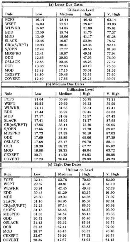
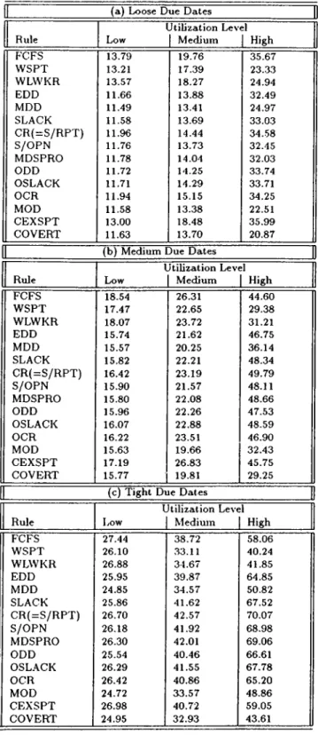
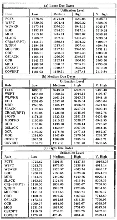
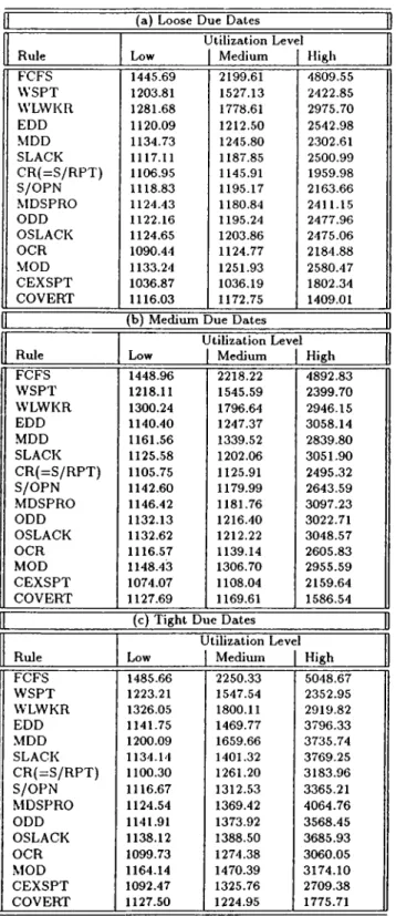
In this study, we consider the dynamic job shop (JS) problem with a pri­ mary performance measure as average weighted tardiness (WT). The results of number of tardy jobs (or percent of tardy jobs, PT) and average conditional weighted tardiness (CWT) are also reported in this chapter. The scheduling environment considered in this study is a dynamic reentrant job shop with the assumptions outlined in Chapter 1. Here, the following additional assumptions are also made:

• Each job has pre-specified routing with randomly sequenced machines and predetermined processing times on each machine in its route;

• Each job is released to the shop upon arrival;

• There is no transportation time between operations;

In addition to these assumptions, the job arrivals are dynamic and a job can visit any machine more than once (i.e., “reentrant shop") but not consec­ utively. The shop contains M machines and each job i has m,· operations with processing times p,j, j = There is a delay penalty, or tardiness weight, of Wi per unit time if job i is completed after its due date d,·. This weight includes customer badwill, cost of lost sales and charged orders and rush shipping costs. Then the W T objective is given by

\V T =

---n

where n is the number of jobs completed during a specified horizon and the tardiness of job i is T, = max {0, C, — d,} in which C, is the completion time of job i. If all the jobs have equal weights, then the objective function becomes unweighted (mean) tardiness. If the objective is to minimize P T, then we consider

i ; < № )

P T = 1 = 1 X 100

n

where ¿(T,) = 1.0, if T, > 0, and d(T,) = 0 otherwise. The CWT objective can be expressed by

cwr =

N T

where N T is the number of tardy jobs among n jobs (also it can be computed by N T = P T x n/100).

In this study, we compare the tardiness performances of some conventional priority dispatching rules with those of recently developed rules in a simulated JS environment.These rules and their definitions are given in Table 2.1. Our

emphasis will be on the new rules such as Apparent Tardiness Cost (АТС) and Bottleneck Dynamics (BD). The long run performances of different versions of АТС and BD are tested. Inserted idleness methods and different resource pricing schemes are studied for the first time in a dynamic .JS environment. The next section reviews the relevant literature on the .J.S scheduling problem along with the discussion of the priority dispatching rules tested. Section 2.3 gives the system considerations and experimental conditions. Computational results are presented in Section 2.4. The chapter ends with concluding remarks in Section 2.5.

2.2

L iteratu re R ev iew

As discussed in the previous section, there are a number of scheduling rules in the literature some of which are listed in Table 2.1. Most of them are simple, known and used for many years. In this section, these rules are reviewed in detail.

2.2.1

C o n ven tion al P rio rity D isp a tch in g R ules

The priority dispatching rules used in the dynamic job shop scheduling are classified by Ramasesh [51] according to the information content of the rules as follows:

• arrival times (e.g. FCFS, etc.) • processing times (e.g. SPT, etc.)

due date information

- allowance-based (e.g. FDD, etc.) - slack-based (e.g. SLACK, etc.)

• cost or value added (e.g. Maximum weight, etc.)

• combination of one or more above (e.g. WSPT, MOD, ODD, OSLACK, etc.)

.Among these rules, FCFS is generally used as a benchmark in the literature. A flow allowance of a job is the time between the release date and the due date, Ai = d,· — r,·. Under the allowance-based priority rules, the remaining allowance of a job i is calculated as A,(i) = di — t at time t. Since t is the same for all waiting jobs at a dispatching decision point, the simplest version of the allowance based priority is the earliest due date rule (EDD). The global slack time of a job is the remaining time for the waiting after remaining work is deducted from allowance. Hence, the global slack of job i waiting for operation

j is Sij{t) = Ai{t) — Pij where is the total remaining processing time or remaining work from current operation j to the end of the last operation. The simplest slack-based priorit}'^ rule is the minimum slack time rule (SLACK), which gives priority to the smallest Sij{t).

The ratio-based priorities use some forms of a ratio for their implementa­ tion. For instance critical ratio rule (CR) assigns the highest priority to the job with the smallest Ai{t)/Pij. While Rohleder and Scudder [52] and Scud- der, et al. [54] show that the CR rule performs well for the net present value objective in the forbidden early shipment scheduling environment, Kim and Bobrowski [32] find out that CR is a good performer in job shop scheduling with sequence-dependent setup times. Another ratio-based rule is slack per remaining processing time (S/R PT) with the priority index Sij{t)/Pij. The priority index of the slack per remaining operation rule (S/OPN) is calculated as Sij{t)fm.ij, where is the remaining number of operations from operation

j to the last operation. The S/R PT rule sees the job with longer remaining

processing time more urgent, while the S/OPN rule gives higher priority to the job with more number of operations remaining. Also we notice that S/R PT schedule is equal to the CR schedule in the sense that their priority indexes yield the same sequence, i.e. S/R P T ij{t) = CRij{t) — 1.0.

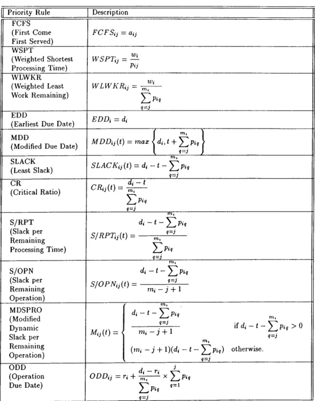
Table 2.1: Priority dispatching rules. (The priorities are calculated for job i waiting for operation j at machine k at time t)

Priority Rule Description FCFS (F'irst Come First Served) FCFS ij = aij WSPT (Weighted Shortest Processing Time) WS PTi j = — Pij WLWKR (Weighted Least Work Remaining) WLWKRii = _m,Wi ^=J FDD

(Earliest Due Date) EDDi = di MDD

(Modified Due Date) MDDij{t) = max < d,·, t +

E

g=j

SLACK

(Least Slack) SLACKi j{t ) = d i - t -

E

9=J

CR

(Critical Ratio) CRijit) =

¿P··« __________g=j S/R PT (Slack per Remaining Processing Time) t ^ ^ Pig S/RPTi j{t ) = ---^ <7=; <I=J _m, S/OPN (Slack per Remaining Operation) S / OPNij {t) = 9=J m - j + ^ MDSPRO (Modified Dynamic Slack per Remaining Operation) = d i - t - J 2 Piç 1=3 mi - i + 1

(?n, - j + l)(¿i - t - Y^Piq) otherwise.

\{ di - t - ^ 2 Piq > 0 mi <I=J <1=J ODD (Operation Due Date) di - r, ^ ODDij — X / J Pig <i=J

Priority dispatching rules (cont’d)

Priority Rule Description OSLACK (Operation Slack) O SL ACK ij [ t) = i-j + ^ - P<;

E

MODij{t) — max < _{7^^--- X} di — Tj V—_{2^Pi q J +Pi j}>

¿ P < î

q=j

CEXSPT (See Note 1) COVERT (Cost Over Time) 'll) · C O V E R T i A t ) = — X Pij f mi / m, ^ i=; V 9=j <1=3 ATC (Apparent Tardiness Cost) tl) * A TC iA t ) = — x exp Pij d i ^ ^ i } ^ i q d · P i q ) P i j ~ t i=;+i KPiavg Wi X exp I I V \ - E ~ ^ I

V ?=j-n

________ /_

(Bottleneck Dynamics) BDij{t) =

/

<1=3

Note 1: CEXSPT rule partitions the original queue into 3 queues which are late queue, i.e. Sij{i) ^ di — t - Y^'^ljPiq < 0, operationally late queue (behind the schedule), i.e.

Oij(t) = dij - 1 - Pij = r,· + ^ X Y^g^i Piq - 1 - P i j < 0, and ahead of schedule queue,

i.e. Oij{t) > 0. Then the rule selects SPT job from queue 1, if this job does not create a new late job with Sij{t) < 0. If it does, then a new SPT job is selected from queue 2, if it does not create a new operationally late job in queue 3. If it does, then a new SPT job is selected from queue 3.

However, the ratio-based priority rules have also some drawbacks in im­ plementations, because negative ratios are difficult to interpret. When the remaining allowance or slack time is negative, these rules behave contrary to their intent. For example, the intent of the S/OPN rule is to give relatively higher priority to jobs which have more remaining operations because they will encounter more opportunities for queuing delay. But, when the slack is negative it tends to misbehave by giving priority to jobs with few remaining operations. For these reasons, Kanet [27] solves the “anomaly” in S/OPN rule by proposing modified dynamic slack per remaining operation rule (MDSPRO) as

i s,At)

MDSPROij{t) =

TTlij if Sij{t) > 0

mijSij{t) otherwise.

Then the MDSPRO rule selects the job with the smallest index to process. All these rules except MDSPRO are extensively tested in scheduling studies. The results indicate that the rules are sensitive to the conditions of the system. For instance FDD, SLACK, S/R PT perform well in shops with light loads, but deteriorate in congested shops, whereas SPT performs well in congested shops with tight due dates, but fails for date-related criteria in shops with light loads and loose due dates [17], [61].

Another way to use the number of remaining operations is to utilize op­ eration milestones called operation due dates (ODD). ODD breaks up a job’s flow allowance into as many pieces as the number of operations in the job. Al­ though there are several ways of assigning the ODDs, the work content method is found to yield best tardiness measures [5]. In this method, the initial flow al­ lowance of a job is distributed to the operations proportional to the operation processing time. The operational version of allowance-based approach leads to the earliest operation due date (ODD). The same analogy for slack-based approach is the minimum operational slack rule (OSLACK). The operational ratio-based approach is smallest operation critical ratio (OCR). Kanet and

Hayya [28] compare the mean tardiness performances of the rules based on op­ erational values with the job-based counter-parts, and show that operational rules are better than the job-based rules.

Baker and Bertrand [7] develop a dispatching rule known as modified due date (MDD) for the single machine shop. In this rule, a job’s original due date serves as the modified due date until the job’s slack becomes zero when its earliest finish time acts as the modified due date. This represents a combination of EDD and SPT rules. Baker and Kanet [8] extend the idea of the MDD rule to the multi-operation job shop. They use modified operation due date (MOD) which employs the ODDs to e.xpedite the jobs in the system. The MOD of an operation is defined as its original ODD or its earliest finish time, whichever is larger. The rule then gives priority to the job with the smallest MOD. Experimental studies show that MOD outperforms other competing rules such as COVERT, CR, S/RPT, SLACK, and MDD at reducing unweighted tardiness at high utilizations and all but very loose levels of due date tightness. In loose due date case, the S/RPT rule produces very small values of tardiness. Baker [5] conducts some experiments to compare allowance based, slack-based, and ratio-based rules with the modified rules (MDD and MOD). The results show that slack based rules do not offer great advantage over simpler allowance-based rules, and operation-oriented rules perform better on the mean tardiness than job-based rules. The MOD rule is shown to be more robust to the changes in due date tightness and it is superior to the other rules when the due dates are not very loose in which S/OPN or A/OPN yields the minimum tardiness. Christy and Kanet [13] show that MOD is the preferred rule for the mean tardiness criterion in manufacturing systems with forbidden early shipment.

Carroll (1965) designs a dynamic priority rule (COVERT) for unweighted tardiness. The COVERT priority index represents the expected incremental tardiness cost per unit of imminent processing time, or Cost OVER Time. The expected tardiness cost is a relative measure of how much tardiness a job might experience if it is delayed by one time unit. The original COVERT can be converted into the weighted version (COVERT) since its derivation depends on the tardiness costs. Hence COVERT includes tardiness weight as a multiplier.

If job i queuing for operation j has zero or negative slack, then it is projected to be tardy by completion with an expected cost of ги, and priority index Wi/pij. If its slack exceeds some worst case estimate of the remaining waiting time over remaining operations, its expected cost is set to zero. If slack is between these extremes, then the priority linearly goes up while slack decreases. By this way, COVERT chooses the highest priority job. Carroll’s experiments show that COVERT was superior to competing rules such as S/OPN and SPT in unweighted tardiness performance.

Russell et al. [53] examine the sensitivity of the COVERT rule to various operating conditions and performance measures, propose different versions of COVERT for the waiting time estimation, and test its performances (mean tardiness, mean flow time, etc.) with other scheduling rules such as EDD, SLACK, S/OPN, SPT, truncated SPT, MDD, MOD, and Apparent Urgency (AU, the very first version of АТС). The simulation experiments show the superiority of the COV'ERT in terms of mean tardiness and mean conditional tardiness performances.

Shultz [55] propose an expediting heuristic for the SPT rule (CEXSPT) which attempts to lessen the undesirable properties of SPT by controlling the scheduling of jobs with long processing times, and by employing job-based and operation-based due date information to expedite the late jobs (see Ta­ ble 2.1). Shultz compare CEXSPT with COVERT, SPT, MOD, S/OPN and OCR. CEXSPT and COVERT produce lower unweighted tardiness values ex­ cept very loose due date case where S/OPN yields the lowest. CEXSPT is the second best rule to SPT and COVERT at minimizing mean flow time and unweighted conditional tardiness respectively. In terms of proportion of tardy jobs, MOD and S/OPN yield the lowest measures at loose due dates, while SPT shows very good performance when the due dates are tight. Ye and Williams [67] explore the CEXSPT rule and make some improvements on it.

2.2.2

АТС S tu d ies

Morton and Rachamadugu [40] develop a priority dispatching rule for the sin­ gle machine WT problem, called “Apparent Tardiness Cost (АТС)" or R&M. The priority rule compares the slack of a job with a multiple times the average processing time of the waiting jobs, pavg- The multiplier is look ahead parame­

ter, K, which represents the average number of competing critical jobs. АТС

gives maximum priority io,/p, (WSPT) if the job has negative slack, whereas it gives a portion of WSPT according to the slackness of the job if it has pos­ itive slack. Its priority increases with decreasing slack exponentially as in the following formula

{di - Pi - t)+\ XJO '

ATCiit) = — X exp \ —

Pi Kp,avg

where (x)'*' = max {0, a:}.

The look ahead parameter, K, can be adjusted to reduce WT costs with changing utilization of the system and according to the due dates tightness level. Morton and Rachamadugu [40], Ow [46] and Vepsalainen and Morton [60] show that К fixed at 2.0 or 2.5 performs well in single machine and static flow shop scheduling problems.

Vepsalainen and Morton [59] extend АТС by adding tail lead time esti­ mation concept to the rule for the multi-machine job shop problems. They calculate operation due date instead of original due date used in the single machine version of АТС as dij — di — TLij, where TLij represents estimated tail lead time which includes remaining work and remaining waiting times in the downstream operations. This differs from the operation due date of MOD. In MOD, initial flow allowance of a job is allocated to operation lead times in proportion to operation processing times. But in АТС, by considering finished and unfinished operations of the job, the time needed to perform the rest of the job is deducted from the due date.

Although there are several approaches to estimate the lead time, the inves­ tigators prefer to estimate it as a summation of known subsequent operation

processing times and estimates of waiting times for these operations. Estimate of waiting time of job i for operation j at each remaining machine enroute is calculated as proportional to its processing time as

Щ =

bpij-By this way, in multi-operation АТС, the global slack is allocated to the re­ maining lead time, which gives “/oca/ resource-constrained slack'"' as

TTt I

SSij{t) = d i - {Wig -b Piq) - Pij - t.

9 = i + l

The look ahead parameter in multi-operation АТС is selected as 3.0 in the experiments (For a full priority formula, see Table 2.1). In the priority formula, the exponential term is the activity time urgency (marginal cost of delay) if the job is currently scheduled and expected to be completed with slack SSij. By this way the urgency factor is

Uij{t) = exp

Kp,avg

Results of experiments conducted by Vepsalainen and Morton [59] show that АТС is superior to COVERT and other competing rules such as EDD, S/RPT, WSPT for WT and also for the number of tardy jobs criterion.

A simulation study conducted by Vepsalainen and Morton [60] confirms the previous results. They test priority-based estimation and the lead time iteration

(LTI) methods to estimate waiting times along with the “standard” estimation

mentioned above. The former depends on queuing analysis. Priority-based waiting time is shorter for high-priority jobs and longer for low priority jobs in the queue. The latter is an iterative procedure (or multi-pass heuristic) to improve the WT objective: In each iteration, waiting times used in АТС (or COVERT) are obtained from previous iteration and they are used in the next iteration. By this way, by making better lead time estimation, the performance of the rule improves. The procedure is repeated until there is no improvement in the WT measures with last fixed number of iterations. The simulation results show that priority based waiting time estimation does not significantly improve

WT performance. Also it is found that АТС or COVERT with LTI improves the performance of the rules based on standard waiting time estimation up to 38%. But the use of LTI is limited to the cases when the system is static (all jobs are available at the beginning) or when the arrival times and other characteristics of the jobs are perfectly known in advance (The latter case is investigated in Chapter 4). In these cases, the model can be iterated before starting the implementation of the schedule.

Ow and Morton [47], [48] extend АТС to static early/tardy problem for single machine and flow shops. They use this extended version of АТС (EXP­ ET) as an initial heuristic for the neighborhood search to find initial schedule and also as an evaluation function for filtered beam search. In these studies, EXP-ET produces very low early/tardy costs in comparison with the АТС and EDD. In addition, in moderate computation times, EXP-ET is improved by beam search as 15% maximum deviation from optimal value or lower bound found by preemptive relaxation of the problem.

Morton and Ramnath [41] add the inserted idleness concept to the АТС rule. By this way, some active schedules are examined myopically. In the first part of the study, they test this version of АТС (X-ATC) and standard АТС against other dispatching rules in a dynamic single machine shop in WT performance. While АТС outperforms all other rules, X-ATC improves the non-delay АТС performance further. In the second part of the study, they use these rules as a first phase heuristics of neighborhood search and tabu search to generate initial schedules. The results show that X-ATC provides best final schedule after the implementation of these search methods as it was the best performer in the first phase.

Kanet and Zhou [29] develop a decision theory approach (MEANP) con­ sisting estimation of total costs for job shop scheduling problem and test it against COVERT and АТС in single machine case. While MEANP produces low values of unweighted tardiness and fraction of tardy jobs as compared with FCFS, SPT, COVERT, MOD and АТС; COVERT and MOD are found to be better than АТС. They recommend MOD for practical applications since it is

the simplest of the three and it heis no parameters to be estimated.

Bengu [10] analyzes the behavior of the АТС performance for varying values of the look-ahead parameter at different combinations of tardiness factor and due date range. The system considered is a flexible flow line shop. Both deterministic case and stochastic case with machine breakdowns are considered. The results show that К should be larger in both of the cases for small due date range and high tardiness factors. But in this study, while the flexible flow line includes more than one machine and more than one queuing point, the АТС implementation is like a single machine scheduling that produces permutation schedule. This version of АТС does not reflect the dynamic intent of the АТС rule.

2.2.3

B o ttlen eck D y n a m ics S tu d ies

In standard applications of АТС, the only cost that the rule considers is about the processing time information of the current operation of the job. In other words, it is assumed that there is no cost for the other jobs in current queue and downstream machines’ queues. Hence, there is no price for the downstream machines. Also АТС and other rules implicitly assume that the price of capac­ ity exists only when the capacity is fully utilized leading to the conclusion that a machine that is not fully utilized (for example 80%) has zero price. Morton et al. [38] show that this is not true due to the non-stationarity of demand. Con­ sequently, they develop the early version of bottleneck dynamics (BD) which they call SCHED-STAR. The proposed model is a scheduling system which uses cost-benefit analysis to make scheduling decisions based on net present value (NPV) of revenues and costs. NPV objective includes tardiness costs, direct costs, inventory holding costs and revenues from sales. SCHED-STAR calculates each resource prices by busy period analysis [42] and then it gives priorities to the jobs according to the calculated rate of return. The model starts with the initial estimates of prices and lead times. Jobs are released into the system from a pool when its computed rate of return is higher than a pre-specified threshold value. After each iteration the NPV is evaluated, lead

times and prices are reestimated by using waiting times and busy periods in previous iteration and simulation proceeds to the next iteration. By this way the resource price iteration (RPI) and LTI are combined in the same module. They test the model in different types of shops including job shop and in dif­ ferent conditions. SCHED-STAR is the best performer as compared with the different versions of COVERT, CR, and EXP-ET. However, in this study the problem sizes studied are very small. Each problem consists of at most 50 operations all available at the beginning of the scheduling period.

In another study, Lawrence and Morton [35] test resource pricing heuristics with and without LTI in static resource-constrained multi-project scheduling problem with tardy costs. They develop a resource price-based priority rule similar to that of SCHED-STAR by taking into account several resource pric­ ing schemes. They include five types of resource pricing methods. Uniform

pricing assumes that all resources are of equal importance giving them 1.0 as a

resource price. Resource load pricing estimates prices as proportional to total resource load. Bottleneck resource pricing uses OPT-like idea and identifies the bottleneck resource with largest load, and gives it a scaled price 1.0, while other resources are assigned prices of zero. Busy period resource pricing is mainly based on busy period analysis which is developed by Morton and Singh [42].

Empirical resource pricing measures prices by successively relaxing resource

constraints and observing the effects on total tardiness. The change in objec­ tive function gives a relative measures of resource prices. They divide the use of information in activity costing as myopic and global. Myopic costing consid­ ers only prices of current resources which process the current activity and the cost is static. Global costing takes into account all prices of resources which process downstream activities. Global costs are dynamic, and are estimated as the sum of resource costs for all unfinished intra-project activities at current time. The first part of the study shows that global pricing dominates its my­ opic counterparts for all resource pricing rules in WT performance. Five global pricing rules with and without LTI and 20 benchmark rules are run in different experimental conditions. They find out that all pricing heuristics dominate all the benchmark rules, and performances of different pricing heuristics are

statistically indistinguishable. In addition, it is shown in this study that the LTI reduces the WT of all pricing rules by 18% on the average.

Recently, Morton and Pentico [-39] bring together all the pieces of their previous studies and develop a new rule with resource pricing scheme which is called Bottleneck Dynamics (BD). In general, BD is a method which estimates prices (or delay costs) for delaying each possible activity (or operation) and prices for using each resource in a shop. Trading off these heuristic prices (or costs) gives a kind of benefit/cost ratio that can be used to make scheduling decisions.

At a scheduling decision point, for each operation of the jobs in a certain queue, an activity price (AP) is calculated. In BD, the AP of an operation represents the costs saved per unit time by expediting the operation by a unit time. Also there are resource prices for each resources (mainly machines). Resource price gives an estimated extra costs if the resource is breakdown or is used for one time unit. If the resource price of a machine k at time

t is known {Rk{t)) and if the operation j of job i is processed on machine k, then the resource usage of an activity for processing is Rk{t)pij. The BD

principle in such a case is that if a net saving is desired at the end of an expediting decision, then it is necessary to expedite the job on its downstream operations. By this way, its completion time will be smaller. In general, job i has operations j , . . ■, m,· as yet unstarted and that will be processed on machine

k{q)^q = m,. If the current operation j is expedited by one unit time, its total resource usage is over the remaining downstream operations. Hence, the total usage of a job while expediting is given by

nii

Rk { g ) { t ) p i g · q=j

Therefore, the BD priority is calculated by trading off the activity price gained by expediting a job and total resource usage of the job. Then, if we denote the activity price of operation j of job i at time t by APij{t), the BD priority is calculated as

APj(l)

1-j

By this way, BD prioritizes the jobs with larger activity prices, while pe­ nalizing the jobs with longer processing times on bottleneck machines on their route. Next, we discuss the pricing mechanisms.

Activity Pricing

Since AP represents the costs saved per unit time by expediting an operation of job by one unit of time, decrease in customer dissatisfaction can be estimated.

Then AP is directly related to the estimated lateness or tardiness of the job and its weight. Hence, the estimated activity price of operation j of job i that will be processed on machine к at time t is given by

A P i j { t ) = W i U i j { t ) ,

where Uij{t) is a function of estimated lateness and is calculated as in АТС. (In fact, Uij{t) is named as urgency factor, and it leads to that APij{t) takes some portion of weight w,, by ranging between 0.0 and 1.0).

If the expected completion time of job i at time t is shown by Cij{t), then the estimated lateness ELij{t) is calculated as

ELij{t) = Cij{t) - di.

Cij{t) can be estimated by the sum of tail lead time, current operation pro­

cessing time and the current time. Then

C i j { t ) = i - f Pij - f T L i j .

From here, we see that ELij{t) = -S S ij{ t) as in АТС. By this way, ELij{t) can be used in urgency factor calculation as SSij{t) is used in urgency as in АТС. Then,

/ { - E L , , { t ) y \

Uij{t) = exp [

If the estimated lateness decreases, the urgency gets larger. If the estimated lateness is already 0 or negative then urgency factor takes its maximum value as 1.0 (leading to activity price = weight of the job).

Resource Pricing

As defined in the previous sections, the resource price gives an estimated extra costs if the resource is breakdown or is used for a purpose for one time unit. Therefore, if the resource is shut down for some time, all the jobs in the queue and the jobs that will arrive before the next idle status of the machine are delayed. The time between two consecutive idle status of the machine is called “6usy period^ of the machine. Hence, if the resource has some jobs in its queue and new arrivals occur before they are finished, the current busy period is the time up to the point that the resource will become first idle. Then the extra cost to the system is the sum of all activity prices of the jobs in queue plus the activity prices of the jobs that arrive before busy period ends. If there are

Nk{t) jobs in the current busy period of resource k, the fundamental resource

price for resource k can be written as

Nk(t)

R,(t) = ^ APi,{t).

t = l

However, in a real shop, we cannot know exact N(¡{1) and activity prices of the jobs. Also, the price will vary over time and roughly proportional to the current busyness of the resource. Since the resource price is a function of current busy period and it is very difficult to exactly know the busy period, there is a need to estimate the busy period.

Morton and Pentico [39] suggest some alternative ways of implementing busy period analysis in the estimation of resource prices. One of the static and moderately simple methods estimates the long run average busy period by queuing theory approximation. This is as follows: