Robust fault detection by simultaneous observers

'■ : “î* V ·\Τ

···‘-4 Ö 2.

A T H E S IS S U B M IT T E D TO T H E D E P A R T M E N T O F E L E C T R I C A L A N D E L E C T R O N IC S E N G IN E E R IN G A N D T H E IN S T IT U T E O F E N G IN E E R IN G A N D S C IE N C E O F B I L K E N T U N IV E R S IT Y IN P A R T IA L F U L F IL L M E N T O F T H E R E Q U IR E M E N T S F O R T H E D E G R E E O F M A S T E R O F S C IE N C E

By

1 ) 5 5 7 ^

U02.

f t u b XQOO

I certify that I have read this thesis and that in rny opin­ ion it is fully adequate, in scope and in quality, as a thesis for the degree of Master of Science.

i t

Prof. Dr. A. Bülent ÖZGÜLER (Principal Advisor)

I certify that I have read this thesis cirid that in my opin­ ion it is fully adequate, in scope and in quality, as a thesis for the degree of Master of Science.

Prof. Dr. M. Erol SEZER

I certify that I have read this thesis and that in my opin­ ion it is fully adequate, in scope and in quality, as a thesis for the degree of Master of Science.

Approved for the Institute of Engineering and Science:

Abstract

This thesis addresses the problem of fault detection and isolation in linear systems based on unknown input observers.

Functional disturbance decoupled observers which estimate specified or un­ specified linear functions of system states regardless of the disturbances are first studied. Necessary and sufficient condition for the existence of such observers are presented. The investigation is extended to simultaneous disturbance de­ coupled observers where multiple systems are observed by a single disturbance decoupled observer.

The application of disturbance decoupled observers to fault detection and diagnosis are explicitly outlined, and a new scheme that is based on simulta­ neous unknown input observers is proposed to enhance the already existing schemes.

Finally, a detailed simulation example is carried out to examine the utility of the proposed scheme.

Keywords: linear systems, unknown-input observers, simultaneous ob­ servers, robust fault detection, fault diagnosis, fault isolation

Bu tezde doğrusal sistemlerde oluşabilecek hataların bulunması, tanınması ve izolasyonu problemleri, bilinmeyen girişli gözleyiciler yöntemiyle İncelen­ mektedir.

Önce bir sistemin durum vektörünün tamamını veya bir fonksiyonunu, bozucu girişlerden bağımsız olarak, gözleyebilen bilinmeyen girişli gözleyiciler incelendikten sonra, buradaki sonuçlar birden fazla sistem için tek gözleyiciden ibaret olan eşzamanlı gözleyicilere genellenmiştir.

Bilinmeyen girişli gözleyicilerin hata bulma, tanıma ve izolasyonuna nasıl uygulandığı özetlendikten sonra, orijinal bir katkı olarak, eşzamanlı bilinmeyen girişli gözleyicilerin bilinen hata bulma yöntemlerinde sağlayacağı kolaylıklar gösterilmektedir.

Bu yeni sonuçların uygulamadaki yararları bir simülasyon örneğiyle ayrıntılı bir şekilde gösterilmiştir.

Anahtar Kelimeler : Doğrusal sistemler, bilinmeyen girişli gözleyici, eşzam,anh gözleyici, hata bulma, hata tanıma, hata izolasyonu

Acknowledgements

I am grateful to Prof. A. Bülent ÖZGÜLER for introducing me to this field of research and for guiding me to accomplish this work. But I am most of all grateful to Prof. A. Bülent ÖZGÜLER for his endless support, patience and comprehension.

I am grateful to the members of the defense committee: Prof. Ömer MORGÜL and Prof. Erol SEZER for their time to read rny thesis.

Special thanks go to Prof. Erol Arkun for his unforgettable assistance and care.

I would like also to thank my friends Mohammed Khames, Nebil Jrriel, Khaled Ben Fatma and Karim Saadaoui for their help and friendship.

Thanks also to the crew of ’’ New York On Air” : Sabeur Aguir, Dale Susani and others for helping with the defense of this work from New York.

Finally I would like to dedicate this work to my parents as a partial acknowl­ edgment for their love and support.

1 IN TR O D U C TIO N 1

2 U N K N O W N -IN P U T OBSERVERS 4

2.1 Disturbance Decoupled O b servers... 5 2.2 Full-State D D O ... 8 2.3 Unspecified Function of S ta te s ... 10

3 SIMULTANEOUS U N K N O W N -IN P U T OBSERVERS 17

3.1 Simultaneous D D O ... 18 3.2 Simultaneous DDO with Common Function of S t a t e s ... 21

4 ROBUST OBSERVER-BASED FAULT DETECTION 23

4.1 Mathematical Model of The S y ste m ... 23 4.2 UIO-Based Residual G en eration ... 25

4.2.1 Residual Generation 26

4.2.2 Structured R e sid u a ls... 31 4.3 Fault Detection and Isolation S ch e m e ... 34 4.3.1 Generalized Observer Scheme 35

CONTENTS _vn

4

3.2

4.4

5 SIM ULATION E X A M P L E : A FO U R -TAN K SYSTEM 41

5.1

5.2 FDI System D e sig n ... 44

5.2.1 System Configuration... 44

5.2.2 Observers D e s ig n ... 44

5.3

52

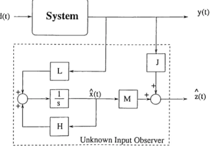
2.1 Structure of a Full-state D D O ... 8

3.1 Simultaneous D D O ... 19

4.1 Diagnostic System M o d e l... 25

4.2 Residual G en era tor... 27

4.3 General Structure of UIO S c h e m e ... 34

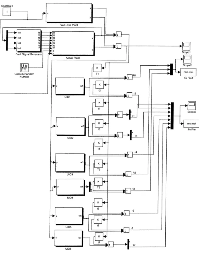
5.1 Four-Tank System 42 5.2 Four Tank System 45 5.3 Overall Simulink M o d e l... 53

5.4 Actual Plant M o d e l... 54

5.5 Fault-free Plant M o d e l ... 54

5.6 Simultaneous UIO No.l M o d e l... 54

5.7 Fault Signal G e n e ra to r... 55

5.8 Output Difference of Actual and Fault-free P la n t s ... 56

5.9 Generalized Residual Response to Single F a u lt ... 57

5.10 Generalized Residual Response to Multiple F a u lt s ... 57

5.11 Residual Vector R(t) Response to Multiple F a u lt s ... 58

Chapter 1

INTRO DUCTION

There has been great concern about improving the process supervision tech­ niques in industrial control applications in order to meet the growing demands for the reliability and safety. These demands are in fact amplified by the in­ creasing complexities and interlinkage of industrial processes as well as the growing scopes of automation and the high capital investments in such pro­ cesses. The motivation is to detect and locate (isolate) the unexpected and unperrnitted process deviation, the so-called fault, from the standard condi­ tions and then take the necessary control action to stop the expansion of the fault and to avoid possible damages to the whole plant such as instabilities and degradation in performance, not to mention the possible hazards to the personnel and the economic losses[l].

The problem is approached by introducing system redundancies whether physical, which are obtained through the repeated hardware elements, or ana­ lytical, which are contained in the static and dynamic relationships among sys­ tem inputs and outputs. However, because of the penalties that the hardware

redundancy imposes on the system including the high cost of the extra equip­ ments, their weight and the space needed to accommodate them, newer fault detection and isolation (FDI) approaches are emerging based on the analytical redundancy at the cost of a mathematical model of the physical plant[2, 3, 4, 5]

The basic principle of model-based (analytical redundancy-based) FDI, is the comparison of the actual behavior of the plant with an anticipated behavior generated with the help of the mathematical model of the same plant. Gener­ ally speaking, the FDI schemes of this type involve two stages: the generation of residuals and the analysis of them. Residuals are functions that are accentu­ ated by faults. They carry relevant information exploited to extract the fault type, source, time of occurrence etc., the kind of data to isolate the fault.[2, 6]

There is a broad spectrum of model-based procedures used for FDI, which can be brought down to parity space approach [7], dedicated observer approach [14, 15, 18] fault detection filter approach [8, 9, 10, 11, 12] and parameter identification approach[3, 13]. The most effective and popular among all is observer-based approach.

In the observer-based approach, the difference between the actual and the estimated system outputs is chosen as the residual. The residual is zero as long as the system is operating fault-free and nonzero when a fault takes place. The underlying assumption is that the mathematical model is a faithful represen­ tation of the physical system. In practice, this idealized assumption is never met because of the system parameters’ variation, modeling error, noises and other disturbances. As a result, there is always a mismatch between the actual and estimated outputs even in the absence of faults. Clearly, this creates a source of false alarms and corrupts the performance of the FDI system. These

CHAPTER, 1. INTRODUCTION

difficulties lead to the robustness issue recognized by [6, 19, 20, 22].

In order to ensure a robust FDI scheme, the FDI system should be de­ signed to be sensitive to faults of interest and at the same time insensitive to other system discrepancies. These conflicting goals are achieved by employ­ ing unknown input observer (UIO), a tool to discriminate between faults and disturbances[22, 21, 15]. Unknown input observers are special kinds of Luen- berger observers that continues to estimate system states even when the system input or part of it is unknown [24, 27, 28, 30, 31]. Since the FDI scheme requires the estimation of the system output, which is a function of the state vector, functional UIO seems to be more appropriate for our purpose, especially that the design problem is then formulated under more relaxed conditions[23, 33].

This thesis is devoted to various types of unknown input observers and their application to robust observer-based fault detection and isolation schemes. It is organized as follows. Chapter 1 covers the unknown input observation prob­ lem with special emphasis on the functional UIO. The results achieved by [28] and [33] are restated and alternative, more transparent proofs are provided. Chapter 2 examines simultaneous unknown input observers and provides some new sufficient conditions for their existence. The objective of Chapter 3 is to give an explicit description of the different aspects of UlO-based FDI schemes and to introduce the simultaneous UlO-based FDI. Finally, in Chapter 4 a sim­ ulation example is considered to illustrate the design procedure and highlight the applicability of simultaneous UIO for the purpose of FDI.

U N K N O W N -IN P U T

OBSERVERS

In the classical observer theory of Luenberger, [25], the states are reconstructed or estimated from measurements of the outputs as well as the inputs. Unknown- input observers, [27], [26], reconstruct the states from the measurement of the outputs only. A main need for unknown-input observers arises whenever some disturbances unavailable for measurements influence the system. The distur­ bance inputs may also be superficially introduced into the model in order to summarize the effect of modeling errors or to represent unaccountable noises influencing certain state variables. In such applications, the unknown-input observers are also designated as “disturbance-decoupled observers (or estima­ tors)” , [35].

In this section, we first review the theory of (linear) functional disturbance decoupled observers. The full-state unknown-input observers are examined as a special case of functional observers.

CHAPTER 2. UNKNOWN-INPUT OBSERVERS

2.1 Disturbance Decoupled Observers

Consider a linear time-invariant system in state-space representation

■^x = Ax{t) -I-

y{t) = Cx{t) -\- Dd{t), z{t) = Ex{t) + Fd{t),

(1)

where x G R " ,d G R ',y G R^ are the state vector, the disturbance vector, and the output vector, respectively. The vector z G R*^ is a function of states and disturbance inputs and we are interested in estimating its value from a knowledge of y. The matrices A, B, C, D, E, and F are known matrices. The problem is to determine a system, called observer, of the form

|x· = H x { t ) L y { t ) ,

z{t) = Mx{t) + Jy{t), (2)

such that the reconstruction error e{t) = z{t) — z{t) satisfies the following conditions:

(i) e(i) is independent of d{t), and

(ii) /imt_>oo||e(i)|| = 0 for all initial states 2:(0) , x (0).

The observer (2) is called a functional disturbance decoupled observer (DDO) for (1) provided (i) and (ii) above hold. Figure 1 illustrates a func­ tional DDO scheme in transfer matrix representation.

x(0)

Notice that, the control input, which is assumed to be measurable, is omit­ ted in (1) and the observer (2) does not use the control input. This causes no loss o f generality since the more general case can be reduced to the above simpler case by redefining the output y{t) to include the control inputs as well, see [28]. A rigorous treatment of the problem based on the frequency domain methods is presented in [28]. A necessary and sufficient condition for the exis­ tence of a functional DDO is given below. We supply an alternative proof of this result of Hautus as the proof in [28] is rather indirect.

P r o p o s itio n 1.1. There exists a functional DDO for (1) if and only if there exist stable proper rational matrices X{s), F (s) such that

- X ( s ) Y{s) ' A - s i b ' — ' E f '

C D _ (3)

P r o o f. We first note that the sought observer (2) can be restricted to be canonical (controllable and observable) without loss of generality. Taking the Laplace transform of e{t) (with initial conditions), one gets

e(s) = [ E - T (s )C ](s / - A)-^x{0) - M { s l - H)-^z{0) + [G(s') - r(s)Z (s)]J(s·),

where e{s),d{s) are the Laplace transforms of e{t),d{t), T (s) := M { s l — H)~^L -f J is the observer transfer matrix, and Z(s) := C{ s l - A)~^B -t- D, G{s) := E { s l — A y'-B + F are the transfer matrices of the system from d to y, z, respectively. The requirements (i) and (ii) are equivalent to

(a) G { s ) ^ Y { s ) Z { s )

(b) E - Y { s ) G = X { s ) { s l - A),

(c) X (s ) and M ( s l - H y'· are stable rational matrices.

Since {H,L) is controllable, it follows that M { s l - W )“ '· is stable rational if and only if

y(.5·)

holding for some stable proper rational matrices X (s)) ^(*')· Note that given any stable rational solution X (s),]h (s‘) of (3) with F (s) proper, a canonical realization of F (s) is a functional DDO (2). □

The equation (3) involves the (polynomial) system matrix

CHAPTER 2. UNKNOWN-INPUT OBSERVERS 7

S{s) := A - s i B

C D

and the question as to “when an appropriate solution to (3) exists” need to be answered. There are at least two alternative answers. One answer is provided by the geometric approach. The problem of disturbance decoupled estimation of [34], [36], [35] is precisely the functional DDO for the special case F = 0, the case where the outputs to be estimated are linear combinations of states only, and for D = 0. The condition for the existence of a functional DDO with F = 0 and D = 0 is that

n K e r C C K e r E , ₍₄₎

where T>1^ ^ denotes the “smallest detectability subspace containing Jm B ” which is the dual space of the smallest stabilizability subspace contained in K e r C , see e.g. [36]. A second approach is to transform the equation (3) to a linear matrix equation over the ring of stable proper rational functions and thereby obtain a condition for its solvability in terms of “unstable invariant zeros” of S{s), see e.g. [37]. Both of these methods provide the valuable intuition that the interaction of the unstable invariant zeros of the system with the matrix on the right hand side of (3) determines whether or not a functional DDO exists. One can state more precise conditions in some special cases. One such case is considered next.

2.2

Full-State DDO

If, in (1), one lets E = R, F = 0, then z{t) = x{t) and the output z of (2) is an estimate of the states of the original system whenever the conditions (i) and (ii) hold. The observer (2) is then a full-state DDO. According to Proposition

d(t) y(t)

z(t)

Figure 2.1: Structure of a Full-state DDO

1.1, a full-state DDO exists just in case (3) holds with E = I , F = 0, i.e., the equation

- X ( s ) y (s ) A - s i B

C D In 0 ] (

5

has a proper stable rational solution [—A'(s') F (s)]. It is not difficult to see that if (5) is satisfied for some stable rational AT(s), F (s ), then

rank -s in + A B = n + rank ' B '

C D D Vs G C, Re{s) > 0. (

6

If X (s ), F (s) are moreover proper, then writing F (s) = Fq -t- K_iS ^ -I-..., one obtains from condition (a) that YoD - 0, VqCB -f- V -iD = B, or equivalently.

^0 P -l

CB D

CHAPTER 2. UNKNOWN-INPUT OBSERVERS It follows that rank OB D D 0 rank OB D r D 0 = rankD + rank B 0 _ -B D (7 )

Hence, if (5) has a proper stable rational solution [—X (s ) F (s)], then (6) and (7) hold. In [28], the converse is also shown. The following is Theorem 1.12 of [28].

P r o p o s itio n 1.2. There exists a full-state DDO for (1) if and only if (6) and (1) hold.

Let us assume, without loss of generality, that the matrix [B' D 'f has full column rank. Then, the condition (6) is equivalent to the system {A, B, 0 , D) being left invertible (i.e., Z{s) has full column rank over R (s )) and all its invariant zeros (i.e., roots of the largest invariant factor of its system matrix S{s)) being in the open left half complex plane. Alternatively, (6) is equivalent to the system matrix S{s) having a stable left inverse. The condition (7), on the other hand, is equivalent to S{s) having a proper left inverse. Finally, the conditions (6) and (7), together, are equivalent to the existence of a proper stable left inverse for the polynomial system matrix S{s).

The geometric solvability condition (4) specialized to E = I (and F = 0, D = 0) becomes:

An alternative condition is due to [22]: A full-state DDO for (1) with E = I , F = 0, D = 0 exists if and only if

(?) rank CB — rank B,

(ii) (C, Ai) is a detectable pair,

where Ai := A — B{CB)'^CA with (CB)'^ denoting a Moore-Penrose inverse of CB. Note that the first condition (?) is eciuivalent to (7) under D = 0. The condition implies in particular that rank B < rank C which means that the number of disturbances that can be decoupled cannot exceed the number of independent measurements. The condition (??), on the other hand, can be shown to be equivalent to (6) and means that the invariant zeros of {A, B, C) are all stable and the system is left invertible.

In the literature, considerable other work is devoted to the design of full- state unknown-input observers using procedures such as system inversion or singular value decomposition, [30], [31]. Whatever method is applied, the re­ strictive existence conditions for full-state observers limit their use in many applications.

2.3

Unspecified Function of States

Full-state DD O ’s suffer from stringent existence conditions. Fortunately, in many applications, not all states are required, rather certain states or certain combination of the states are enough to fulfill the task, [32], [33]. Moreover, in fault detection applications, it is even enough to focus on functional unknown- input observers which estimate some (a priori unspecified) function of states.

CHAPTER 2. UNKNOWN-INPUT OBSERVERS 11

Given a system

= Ax{t) + Bd{t),

y{t) = Cx(t) + Dd{t), (

8

the problem of functional DDO with unspecified E is to determine a function of states

z{t) — Ex{t), E 0 ₍

₉

and a disturbance decoupled observer (2) as in the previous section. The significant difference from the problem considered in Proposition 1.1 is that F — 0 and the matrix E on the right hand side of equation (3) is now also an unknown and is to be determined. It is easy to see by similar reasoning that lead to Proposition 1.1 that the problem of functional DDO with unspecified E has a solution if and only if there exist stable proper rational matrices X{ s) , Y{s) and a constant nonzero E satisfying

[ -A -(s ) r ( s ) ] A - s i B

C D = [ i o ] . (10)

A simple condition for solvability for the problem has been obtained in [33] using ideas from the theory of descriptor (generalized) systems. We now state this result and give an alternative proof using more elementary notions.

P r o p o s itio n 1.2. There exists a functional DDO with unspecified E for the system (8) if and only if either one of the following conditions hold:

(i) rank C D > rank D.

P r o o f. Let t /(5),L (s ) be some unirnodular polynomial matrices such that U{s)S{s)V{s) = A(s) is the Smith normal form of S{s) over the ring of poly­ nomials. Let A = AsAa be a stable-antistable factorization of A with A^ square, nonsingular. Thus, det As{s) includes among its zeros all zeros of A in the strict left half complex plane and only these.

[If] Suppose (i) in (11) holds. Then, there exists J e for some A; > 1, such that J C ^ 0 and JD = 0. Let E = JC, X{ s) = 0, F (s) = J. Then, (10) is satisfied. This shows that if (?) holds, then a constant DDO exists. If (m) in (11) holds, then A~^U is stable rational, non-polynomial, and satisfies Aj^US = AaI/“ L Partitioning A~^U = [ —X Y ] with X having n columns, we have

X { s l - A) + YC

- X B + Y D = T2, (12)

for some polynomial matrices T i , T2. Let us write X = X+ -\- X _ , where X - = X -is X -i-iS ^ -f-..., X_i / 0, and I > 1. Multiplying each term in (12) by and taking the strictly proper part of each term gives

{ V - C X ) 4 s I - A ) + { s^- W) _C = X_i, { V- ^X) _B = { V - W ) . D .

Since E ·.— X_i ^ 0, (10) is satisfied and (s^~^F)_ is a transfer matrix for a DDO. Note that the poles of (s^“ ^F)_ are among the roots of det As which are the stable invariant zeros of the system matrix S{s).

[Only if] Conversely, suppose there exists a DDO so that for some X (s ),F (s ),£ ^ ^ 0, (10) holds. We assume, without loss of generality, that in (10) [C D] has full row rank. If not, by appropriately redefining F(.s), a

CHAPTER 2. UNKNOWN-INPUT OBSERVERS 13

similar equation with the assumption fulfilled can be obtained. We have

- X Y U~^AsAa= E 0 V

Let us first suppose that S, and hence Aq, has full row rank. Let —X Y U~^ = 0r~^ be a right coprime polynomial factorization, where d etr is a Hurwitz stable polynomial since —X Y j U~^ is stable rational. It follows by left coprimeness of 0 and F and by the fact that 0r~^A5Aa is polynomial, that A^Aq = Fd^ for some polynomial matrix Therefore, either F and As have a nontrivial common left factor implying that A^ has a stable invariant zero, so that (ii) in (11) holds, or F is unimodular implying that - X Y is constant. In the latter case, since X = Y C { A — sl)~^ is strictly proper, we must have X = 0. This gives that E = Y C ^ 0 and Y D = 0 which implies (i) in (11).

Suppose next that the system matrix S is not of full row rank. Let

- 0 T be a minimal polynomial basis, [38], for the left kernel of S, i.e..

[

- 0

^

C D

= 0,

where, by 0 = ^ C { s l — A) ,

deg Oir < deg i = 1, (13)

with 0jr, 'Fi,· denoting the of the matrix 0 , \k respectively. Let A ;= diag{ai, ...,ak} for Hurwitz stable polynomials satisfying degai = deg'^i for i = 1,...,A:. Then, X := A " i 0 , r := (A -^ T )_, and E := -(A -H F )oC' are such that (10) is satisfied. By the degree condition (13), X is strictly proper so that (A “ HI/)qT) z= 0. Further, by the definition of a minimal polynomial

basis, is of full row rank. If = 0, then (A “ ^'3/)o[C'Zi>] = 0 which, by our assumption that [C D] has full row rank, is not possible. Hence, E — — (A“ Hlf)Q(7 ^ 0 whereas — q. It follows that (z) in (11) holds. □

Note that the argument in the last paragraph of the proof also establishes the fact that “If

ranik S < n + rank \^C Z) ]

(or, if [0 D] has full row rank but S has a row defect), then a constant DDO exists” . A closer examination of the construction parts in the proof yields the following facts stated without proof.

C o r o lla r y 1.1. Suppose [0 D] has full row rank. There exists a DDO with unspecified E which

(i) is constant if and only if rank ^ C Z) j > rankD,

(a) has any set of desired stable poles if and only if the system matrix S does not have full row rank.

If the system has a stable invariant zero, then there exists a DDO with unspecified E with poles a subset of the stable invariant zeros of S.

Let us now consider the following example which shows that the trivial case where Y(s) = 0 is a disturbance decoupled observer transfer function must be considered as an observer with fixed dynamics.

E xa m p le. Consider the system.

A = - 1 0 0 1

, B = 0

1

0

1

CHAPTER 2. UNKNOWN-INPUT OBSERVERS 15

Then, the observer K(s) — 0 and the choice E \ 0 satisfy the reciuire- rnents from a DDO with unspecified E. For this data, D is nonsingular so that, by Corollary 1.1, a constant observer does not exist. On the other hand.

/ 1 - s · / D

C D

is nonsingular so that, again by Corollary 1.1, an observer with assignable poles does not exist. Therefore, Y(s) = 0 must be treated as a case with “fixed dynamics” in spite of the fact that this causes an abuse of the term since 0 can be considered to have any stable denominator.

The trivial solution F (s) = 0 can be avoided by assuming that {A, B) is controllable. To see this, let M ( s ) , N (s), N (s), M{s) be polynomial matrices such that M{ s ) , M{ s ) are nonsingular.

U(s) : = [ A - s / B M{s) - N { s ) N{s) M{s) is unimodular, and ' M(s) - N { s ) ' ’ / o ' N{s) M{s) (14)

Such matrices exist by controllability of {A, B), [40]. Multiplying both sides of (10) on the right by U{s), and supposing

y(s)

The assumption of controllability of {A, B) leads to a further simplification in (10).

functional DDO with unspecified E for the system (8) if and only if there exists a proper stable rational matrix Y(s) and a constant E 0 satisfying

E - Y { s ) { s i - A)-^B

C { s l - A)-^B + D =

0

P r o o f. By controllability of (8), there exists a unirnodular U{s) as in (14). Multiplying both sides of (3) on the right by U and using (14), we obtain Y{ s) [ DM{ s) - CN{s)\ = - N { s ) E . Since, from (14), N{ s)M{s)- ^ = - { s i - A)-^B, we have P(s)[C'(s·/ - A)~^B + D] = E { s l - A)~^B and (15) holds. Conversely, if (15) holds for a proper stable Y(s) and constant nonzero E, then let X (s ) := Y{ s) [ CM{ s) + DN{s)] — EM{ s) which is stable rational. By (15), we also have Y{ s) [ DM{ s) — CN{s)\ — —N{ s)E. Combining the two, we have

- X ( s ) Y{s) A - s i B U{s) = [ ^ 0 ] U{s)

which gives (10) for a proper stable rational l^(s) and a stable rational X{s). However, X{ s ) = [E — Y{s)C]{sI — A)~^ and properness of P (s) implies that X (s ) is also proper (actually, strictly proper). □

Chapter 3

SIMULTANEOUS

U N K N O W N -IN P U T

OBSERVERS

The idea of simultaneous observation can at least be traced back to [39]. It is concerned with the design of a common observer for a given set of two or more systems. Such a set of systems may result from a plant undergoing changes in its structure or in its parameters as a result of changes in operating con­ ditions. It may also be a set of linear models matching a nonlinear system closely at various operating points. In the latter case, the simultaneous ob­ server, whenever it exists, can be considered an approximate linear observer for the nonlinear system. Although the problem of simultaneous stabilization has been intensively examined, see e.g. [41], the dual problem seems to have attracted less attention. In [43] and [42], the problem of simultaneous observers has been investigated using coprime factorization techniques: [4.3] takes a sim­ ilar approach to that of [41] and reduces simultaneous functional observation problem of r 4-1 plants to the same problem for r auxiliary plants. Conditions

for the existence of a simultaneous observer for two plants are obtained but they are conditions on transformed data. In [42], the focus is on obtaining a parametrization of all simultaneous functional observers for a set of plants and this has been done under a rather severe restrictive assumption of the existence of a stable left inverse for a composite plant. This assumption can easily be shown to be equivalent to the assumption that the plants admit a simultaneous

“full-state” observer.

In this section, we investigate the conditions for existence of functional simultaneous unknown-input or disturbance decoupled observers. Since our objective is to employ such observers in the design of fault detection and iso­ lation, we are interested in functional observers with unspecified function(s) of states. Although the results below apply to an arbitrary number of systems with appropriate modifications, for simplicity, we will constrain the presenta­ tion to the synthesis of a simultaneous DDO for two systems only. We first consider the general case of simultaneous DDO where the estimation of, in general, different functions of states of the two systems is desired. The results are then specialized to the estimation of the same function of states.

3.1

Simultaneous DDO

Let us consider two linear, time-invariant systems S i and S2 described by the following equations:

El :

xfit) — AiXi{t) -f-

CHAPTER 3. SIMULTANEOUS UNKNOWN-INPUT OBSERVERS 19

and

So ; X2{t) — ^^2X2{i) + 52^2 (i)

y2(t) = C2X2{t) + D2d2{t)

where xi{ t), X2{t) G R " are the state vectors, di{t) G R"'“ ,d2(i) € R"^"^ are disturbance vectors, yi{t),y2{t) G R^ are the measurement vectors of Si and So, respectively, and Ai, A2, R i, Ro, Ci, C2, R i, and D2 are constant ma­ trices with appropriate dimensions. The problem of simultaneous DDO is to determine matrices Tj 7^ 0, '¿ = 1,2 and a functional DDO of the form

X = Hx{t) P Ly{t),z{t) — Mx{t) P Jy{t),

where y{t) is a vector-input to the observer such that the errors

ei{t) = TiXi{t) - w{t), i = 1,2

satisfy the following conditions for = 1,2: Whenever y{t) = yi{t), (i) ei{t) is independent of d{t) and

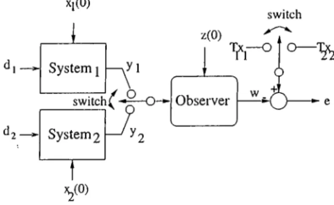
(ii) limt^oo\\ei{t)\ \ —0 for all initial states ^¿(O) and i (0). X[(0) switch z(0) System I y\ switch^ ^Q— y System 2 T “ ^(0) T^J-O Observer J

P r o p o s it io n 2.1. There exists a simultaneous DDO for Ej, i = 1,2 if and only if there exist stable rational proper matrices Xi{s), i = 1,2, Y{s) and constant Ti ^ 0, i — 1,2 satisfying X l ( s ) X 2(.?) r ( s ) yli - s i _{0 P i 0} 0 A2 - s i 0 P2 Cl C2 C l D2 Ti T2 0 0 .(1)

P r o o f. The result follows easily by writing (10) for both Ei and E2 with the same Y(s) and combining the two equalities obtained in one matrix equation. □

Thus, by Proposition 2.1, a simultaneous DDO exists for Sj, i — 1,2 just in case there is a DDO for the combined system

E = ( C l C2

0

P i 0

0 B2 , [ A D2 ])

with a special function of states, i.e. a function [Ti T2] / 0 where Ti and T2 are separately nonzero. Theorem 1.2 applied to E gives that if a simultaneous observer exists, then either the system matrix associated with E has a stable invariant zero or ranA: [Ci C2 Di D2] > rank[Di D 2]· This condition is also sufficient provided the transfer matrices Ej(s) := Cj + {si — Ai)~^Bi + Di have full row rank for i = 1,2.

T h e o r e m 2.1. Suppose the transfer matrices Zi{s) ofEi have full row rank for i —1,2. There exists a simultaneous DDO for Ej, i = 1, 2 and only if rank [Cl C2Di D2] > rank [Di C2] or E has a stable invariant zero.

P r o o f. The “only if” part is by Theorem 1.2. To see the “if” part, suppose either E has a stable invariant zero or the rank condition holds. Then, by Theorem 1.2, there exists a functional DDO for E for some [Ti T2] / 0. We

show that if Tj = 0 for some z = 1,2, then the corresponding transfer matrix has a row rank defect. Suppose Ty = 0. Then, by (1), yYi(s)(yl - s / ) + X2(-5)C'i = 0 and Xi{s)By X2{s) Di — 0. Now, [JYi(s) .^^2(5)] 0 since otherwise in (1) T2 = Y{ s ) C2 = 0 contradicting [Ti T2] ^ 0. It follows that the system matrix associated with Ei has a row rank defect which implies that the transfer matrix

of El has a row rank defect. □

Corollary 1.2 also gives an alternative useful condition for simultaneous DDO in terms of the existence of a left kernel of a special type.

T h e o r e m 2.2. Suppose Ei, z = 1,2 are both controllable. There exists a simultaneous DDO for Ej, z = 1,2 if and only if there exist constant Tj / 0, z = 1, 2, and a stable rational proper matrix T (s) satisfying

CHAPTER 3. SIMULTANEOUS UNKNOWN-INPUT OBSERVERS 21

Ti T2 - Y { s )

{ s I - A y ) - ^ B i 0 0 {sI - A2 ) - ^B2

Ci{sl - Ay)-^By + Dy C2{sl - A2)-^B2 + D2

= 0. (2)

P r o o f. This is a direct consequence of the problem definition and Corollary

1.2. □

3.2

Simultaneous DDO with Common Func­

tion of States

Let us now impose a further constraint that Ty = T2 in the simultaneous DDO sought for Ej, z = 1,2. The eciuation (1) should now be satisfied for some T := Ty = T2. The following counterpart to Proposition 2.1 can be stated.

P r o p o s it io n 2.2. There exists a simultaneous DDO with common func­ tions of states for Ei, i — 1,2 if and only if there exist stable rational proper

matrices Xi(s), i = 1,2, Y{s) and a constant matrix T ^ 0 satisfying X, { s) X

2

2

1

2

2

2

2

2

r 0 0 0

/

It follows that (1) has a solution X i, X2, Y for some T = Ti = T2 if and only if X i , X2— X i , Y is a solution to (3) for that T. □

T h e o r e m 2.3. Suppose the systems S i and S2are both controllable. There exists a simultaneous DDO with a common function of states for Sj, 'i == 1,2 if and only if there exists a proper stable rational matrix Y(s) and a constant matrix T ^ 0 satisfying

T - Y ( s )

C ,{sl - A , r ' B i +

C2(sl - A2)-'B2 + D2

0. (4)

P r o o f. The result is an immediate consequence of the problem definition and

Chapter 4

ROBUST OBSERVER-BASED

FAULT DETECTION

4.1

Mathematical Model of The System

Recalling that the observer based FDI (and the model based FDI in general) involves a comparison between the actual system response and an anticipated system response generated using a mathematical model, the performance of the scheme depends on how faithful the model is to the underlying physical system. The better the model used to represent the dynamic behavior of the system, the better is the chance of achieving a robust fault detection and iso­ lation system. In practice, the system is subject to different uncertainties that if omitted tend to create false alarms and corrupt the system performance. These uncertainties include modeling errors due to system parameter varia­ tions, unknown noise-type disturbances on the system and nonlinear terms in the dynamics. Therefore, the mathematical model should include a realistic description of the uncertainties in the system to be monitored. This kind of

model is known as a diagnostic system model (in contrast to a representative model used for control purposes). In general, a dynamic system subject to faults and system uncertainties may be represented as follows [6]:

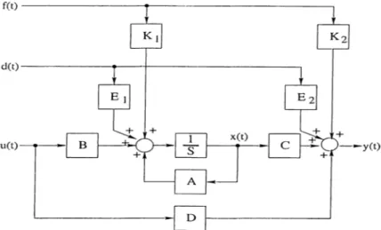
X — (^A + Ay4)a;(f) + ( 5 + A.0)ri(i) + Endi(t^ + / ’f i / ( f ) ,

y{^) ~ AC)x(t) + (D + AD)u[t) + E\2d\{t) + K2f{t), (1)

where x E RL,u G R '” , d^ G R^ / G R^, y G R^ are the state vector, the control input (known), the disturbance vector, the fault vector, and the measurement vector, respectively. The matrices A , B , C , D , En, E12, Hi and K2 are known matrices of appropriate dimensions. The matrices AA, A S , A C and A D are the parameter errors or variations representing the modeling errors. The disturbance and the fault vectors are unknown time functions whereas the fault and disturbance entry matrices , S i, S2, K\ and K2 which represent the effects of faults and disturbances on the system are known. According to [44], the modeling errors can be summarized as additive disturbances E2\d2{t) and E22(t)d2(t) on the states and the outputs, respectively, where E21 and E22 are computed as functions of A A , A S , A C and A S , and where ¿2 is an unknown function of time. We can then write (1) as

X — Ax{t) + Bu{t) + Eid{t) + Ki f {t ) ,

y{t) = Cx(t) + Du(t) + E2d(t) + K 2f{t), ( 2 )

where d{t) = [di(ty d2{t)']' is a new disturbance vector and Ei = [En E21], E2 — [Ei2 E22]· In transfer matrix representation, (2) is

CHAPTER 4. ROBUST OBSERVERM SED FAULT DETECTION 25

Figure 4.1: Diagnostic System Model

4.2

UIO-Based Residual Generation

A residual in the context of FDI is a scalar or vector valued signal that is accentuated by the fault vector. It carries information about the time and location of an occurrence of a fault. It is also independent of the normal operating state of the system.

To avoid false alarms that may be triggered by system uncertainties men­ tioned in the previous section, the residual should be insensitive to such un­ certainties yet sensitive- enough to faults that may occur. In other words, the residual should be chosen so that it discriminates between faults of interest and other disturbances acting on the system. Motivated by the decoupling property of the UIO, most robust residual generation is performed based on UIO. The residuals are chosen as the reconstruction errors of the states of the system which are independent of the unknown uncertainties thanks to the UIO observer. In fact, what interests us in FDI is the reconstruction of a function of states in presence of disturbances and not necessarily all the states. Recall from Chapter 2 that the existence condition for such observers are easier to

4.2.1

Residual Generation

Let us consider a faulty system given by the equations (2) in state-space rep­ resentation and by (3) in frequency domain. Let a general functional observer for this system be given by

x{t) = Hx{t) 3- Ly{t) -f Niu{t), z{t) = Mx{t) -I- Jy{t) -I- N2u{t), (4)

where the matrices H , L , M , N i , N2,J, and T / 0 are to be determined such that the residual

r{t) = Tx{t) — z{t) ₍₅₎

in steady-state becomes zero for the fault-free case and nonzero for faulty cases. Taking Laplace transform of each term with initial conditions a;(0) and i(0 ) yields

f(s ) = [T - Hy{s)C\{sI - 4 )-ia ;(0 ) - M { s l - Hy^x{D) T\T{sI - A)-^E, - Hy{s)Gd{s)]d{s)

+ [T (s·/ - A)-^B - Hy{s)Gu{s) - H^]u[s) + [ T ( s / - A)-^K, - Hy{s)Gj{s)]f{s)

(6)

Here, Hy[s) — M { s l — H)~^L -I- J is the observer transfer matrix from y io w and Hu{s) — M { s l — H)~^Ni q- N2 is the observer transfer function from u to w. We now pose the following requirements:

{i) [T — Hy{s)G]{sI — and M { s l — H)~^ are stable rational,

(n )

T{sI-A)-^E,^Hyis)Gd{s),

CHAPTER 4. ROBUST OBSERVER-BASED FAULT DETECTION 27

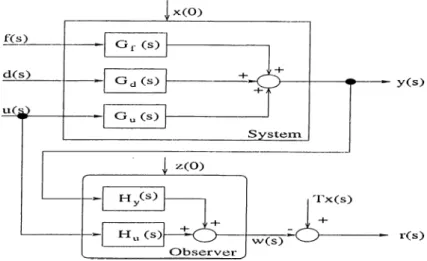
Figure 4.2: Residual Generator

Note, by (6), that (i) — (Hi) hold if and only if

y(s)

r(s)

lirn r{t) = 0 V 2;(0), ¿(0 ); V u(t), d{t).

t—^oo (7)

We now claim that (i) — {in) hold if and only if {H, L, M, J) is a functional DDO for the system {A, Ei,C, E2) for a function Tx{t) of the states. To see this, first observe that the requirements (¿) — {in) can be expressed equivalently by

(a) [ T - H y { s ) C ] = X { s ) { s I - A ) ,

{b) T {sI - A ) - ^ [e, B Ga{s)

I Hy{s) Hu{s)

(c) ^ (5), Hy{s), Hu{s) are stable proper rational matrices.

Since

’

G,{s)

G '

El B

E 2 D

by Proposition 1.2, the requirements (a) — (c) are satisfied if and only if there exist stable proper rational X ( s ) , Hy{s), Hu{s) satisfying

[ - ;i(6 ·) Hy{s) H u { s ) '

which holds if and only if

[ - x ( s ) n w n w ; A - s i El B C E2 D 0 0 I T O O (8) / 1 - s / El 0 C E2 0 0 0

/

is satisfied for some stable proper rational X{s ),Y i{s ),Y2{s). It is now clear that this last equality can be satisfied by ^2(5) = 0, Pi(s) a functional DDO transfer function for {A, B, Ei, E2), and an appropriate yY(s). This proves the italicized claim above. The existence conditions for a functional DDO (4) for the system (2) of this chapter and a DDO (2) for (8) of Chapter 2 thus turn out to be the same. The synthesis procedures are only slightly different. In designing a (4) for (2), one first obtains T / 0 and stable proper X { s ) , Y { s ) such that the equality (10) of Chapter 2 (with E T) is satisfied. Then, Hy{s) = Y{s),Hy,{s) = X { s ) B — Y{s)D will satisfy (8), with the same X (s ) and T, and hence the requirements (a) — (c). A canonical realization of [Hy[s) Hu{s)] is now a functional DDO (4) for (2).

R e m a rk 4.1: Suppose that in our synthesis procedure we neglect the control inputs u{t) altogether and choose a functional DDO {H,L, M ,./), i.e., (4) with Ni — 0, i — 1,2, for the system (2) with T / 0. We know from Section 2.1 that the requirements (i) and (ii) will be satisfied. We check the

requirement (iii). The transfer function

T{.sl - A)--^B - Hy{s)Gu{s) = [ T - Hy{s)C]{sI - A)~^B - Hy{s)D

is stable rational by (?) and by the stability of the observer transfer function

Hy[s). This implies that for all bounded control inputs |wi(i)| < oo, i =

1 , m, the effect on the residual will be bounded at all times and the presence of a fault can still be detected by a change in the steady-state residual value in the presence of a fault.

R e m a rk 4.2: If the system (2) is stable, a common method of taking care of the control inputs u{t) in the literature is canceling their effect on the outputs y{t) at the outset. This requires defining

y{t) ■ = y { ' t ) - y { t ) ,

where y{t) is the output of the “fault and disturbance free system” , i.e., it is the output of (2) with d{t) — 0, f{t) = 0, i > 0. The observer (4) is then replaced by

CHAPTER 4. ROBUST OBSERVER-BASED FAULT DETECTION 29

x{t) = Hx{t) -l· Ly{t), z{t) = Mx{t) -b Jy(i). (9)

The residual r{t) = Tx{t) — z{t) now becomes

f{s) = [ T - Hy{s)C]{sI - A)-^[x{0) - 5(0)] - M { s l - FI)-^x{0) - T { s l - y4)-i5(0) + T { s l - A)-^Bu{s)

+[T{sI - A)-^E, - Hy{s)Ga{s)]d{s)

+ ( T ( s / -

A)-^K, - H,(s)G,(s)]l(s),

where the effect o f the term —T { s l — yl)“ ^5(0) + T {s l — A)~^Bu{s) on r{t) is a constant at the steady-state for bounded control inputs. Note that this

method requires the simulation of a fault-free system model in order to obtain the output y{t). In view of our Remark 4.1 however, this method seems rather pointless since, a functional DDO will provide constant steady-state effects on the residual for bounded inputs anyway.

A residual (6), in addition to (7), must have some further properties to detect and isolate faults;

1. The fault effect must be distinguishable from the effect of disturbances for the purpose of fault detection.

2. The effect of a fault must be distinguishable from the effects of distur­ bances and other faults for the purpose of fault isolation.

We now formally define detectability and isolability of faults with respect to the residual (6).

Suppose that (i) — (Hi) are satisfied for some T 7^ 0 and a functional DDO (4). Then, the residual (6) becomes

f{s) = e(.s) + Grf{s)f{s),

where

e{s) := [T - Hy{s)C]{sI - A)-^a;(0) - M { s l - H)-^x{0), Grf{s) := T { s l - A)-^Ki - Hy{s)Gj{s).

Let [G'r/(s)]i denote the Ath column of the matrix [G'r/(6·)]·

Definition 3.1-Fault Detectability ([21]): A fault fi{t) is said to be detectable if /

0-CHAPTER, 4. ROBUST OBSERVER-BASED FAULT DETECTION 31

Thus a detectable fault signal /¿(i) (from the residual r{t)) is such that

/.(¿) 7^ 0 ^ lim r{t) 7^ 0 c—>oo

for any 2;(0),£ '(0) and for any d{t),u{t). In order for all faults to be detectable through our residual (6), in addition to (a) - (c), we also need to satisfy

[T{sl - A)-^K, - Hy{s)Gf(s)]i 7^ 0 V z = 1, g (1 0)

by an appropriate choice of T 7^ 0 and M, L, J, N1 , N2.

D e fin itio n 3.2-F ault Iso la b ility ([21]): A signal fi{t) is isolable from /2(1) by the residual (6) if

[Grf{s)]i,[Grf{s)]2

are linearly independent vectors (over R (s )). This means that the effect of fault fiif) on the residual is different from the effect of f2{t) since [Gr/(s)]i = [Grf{s)]2{fi{s)/f2{s)) is not possible. Fault isolability is ensured together with fault detectability (by the same residual vector) if Gr/{s) has full column rank over R (6‘), a condition that will not be satisfied in case of a large number of faults. In practice, and in our simulation example of Chapter 5, however, fault isolation is achieved by defining different residuals for capturing different faults as we discuss in the next section.

4.2.2

Structured Residuals

Fault isolation is a more difficult task than just detecting a fault. One approach to fulfill this task is to design a structured residual set— structured in the sense

that each residual is sensitive to a certain group of faults, while insensitive to others. The design procedure consists of two steps, the first is to specify the sensitivity and insensitivity relationships between the residuals and faults, and the second is to design the residual generators that will implement these desired specifications by treating the faults that the residual is insensitive to as unknown inputs (in addition to the already existing disturbances). The advantage of the structured residuals is that the diagnostic analysis is reduced to determining which residuals are non-zero. For each residual, a threshold test is performed separately, yielding a boolean decision table that will serve to isolate the faults taking place.

Given a set a faults /¿(t), (i= l,2 ,...,g), a set of residuals rj(t), (i=l,2,...,g) can be designed according to one the following two types o f structured residuals

Dedicated Residual Set: A set of residuals obeying the following condi­ tion

nit) = Qifi{t));i e { 1 ,2 ,,..,^ } ,

where Q(.) denotes a functional relation. A simple threshold logic can be used to decide about the appearance of a specific fault by logic decision according to:

nit) > Ti fi ^ 0;i e {1, 2,,

where Tj (i = l,2,...,g) are threshold values. If we let g = 4, we get the following table of dependency.

CHAPTER. 4. ROBUST OBSERVER-BASED FAULT DETECTION 33

r2(t)

o{t)

n{t)

fl{t)

f2{t)

hit)

U(t)

In the table above, a “ 1” in ith row and jth column denotes that the residual rj is sensitive to the fault /¿, i.e., depends on it, whereas a “0” denotes insensitivity.

G e n e ra lize d R esid u a l Set: The residuals of this type are generated ac­ cording to the following equations;

ri{t)

Q{f

{t),--Jait))

ri(t) = Qihit ), ···, ··., fg{t))

^git) =

The isolation is again performed using simple threshold testing according to the following logic:

uit) < Ti

rj{t) > Tj 'ij ^ i

Again, if we let <; = 4, we get the following table of dependency.

^lit)

oit)

nit)

nit)

hit)

hit)

hit)

4.3

Fault Detection and Isolation Scheme

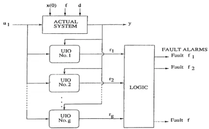
Having addressed and discussed the residual generation problem, we are now ready to introduce UlO-based FDI scheme. Given a faulty system, the basic idea is to use a bank of (functional) unknown input observers to generate a set of structured residuals. The bank of observers, known as observer scheme may generally consist of an arbitrary number of observers, but often equals the number of faults to be detected and isolated[l]. To be more specific, let us assume that g different faults /¿(t) {i = 1 ,2 ,...,^ ) may take place in the system to be monitored. A bank of g (functional) unknown input observers is driven by the control input u{t) and the system output y{t) to generate g residuals Tj(i) {i = 1,2,...^) which in turn drive a decision logic unit responsible for issuing the fault alarms. The system is depicted in the following diagram.

x (0 ) f

Figure 4.3: General Structure of UIO Scheme

The choice of structured residual type that the scheme relies on is deter­ mined by how many faults we want to detect and isolate at the same time. There are two main situations: either only a single fault is to be detected and isolated at a time or all faults are to be detected and isolated even if they occur

simultaneously. In the first case, generalized residuals are used and the scheme is known as generalized observer scheme, while in the second case dedicated residuals are used and the scheme is refereed to as dedicated observer scheme.

4.3.1

Generalized Observer Scheme

The basic assumption underlying this approach is that only a single fault can take place at a given time, which is in practice most probable. To generate the (j residuals, g different systems are formed from the state space equation of the plant (2) by treating one fault as a disturbance at a time. For each of these systems an UIO is designed to decouple the augmented disturbance vector that now includes one of the faults. A set of generalized residuals is then obtained. If a fault fi takes place in the plant, the P'’’ residual is completely invariant to it {ri{t) = 0) , whereas the remaining g — 1 residuals rj{t), j ^ i, carry the fault symptoms. The appropriate evaluation of the residuals reveals the fault.

This kind of detection scheme is accurate and robust because the distur­ bance vector is augmented by only one fault leaving some design freedom to decouple the unknown inputs from the residual and achieve the desired robust­ ness. However, if more than one faults simultaneously act on the system, all residuals will be affected by one fault or another and none of them is zero. In such cases, the scheme collapses.

4.3.2

Dedicated Observer Scheme

CHAPTER 4. ROBUST OBSERVER-BASED FAULT DETECTION 35

In contrast to the generalized observer scheme, the dedicated observer scheme handles simultaneous faults. Again g different systems are formed but this time all faults but one are treated as disturbances in turn. Each of the g UIO’s

is designed to decouple g — 1 faults in addition to the unknown input vector. Therefore any residual rj(i) {i — l,...,g) is sensitive (dedicated) to a unique fault If multiple faults occur in the system, then the specialized residuals will be nonzero while the rest remain unaffected. By considering which residual deviates from zero the faults are detected and isolated. The problem with this scheme is that the augmented disturbance vector is overloaded by faults. In most cases it is difficult to design observers that decouple all — 1 faults. Even if they exist, there will be no design freedom left to reject other I true disturbances influencing the system resulting in a nonrobust EDI system.

4.4

Introducing Simultaneous UIO in FDI

The observer schemes, generalized and dedicated alike suffer from limitations that make it sometimes difficult to design a reliable detection and isolation sys­ tem. In the previous section, we have seen that the former fails to reveal faults that act simultaneously on the system and the latter is not robust enough and is difficult to design. Nevertheless, each of them has its nice features; while the generalized observer scheme is relatively immune against system discrepancies, the dedicated observer scheme is capable of coping with simultaneous faults affecting the system. We want to combine both schemes so that the limita­ tion of one of them is compensated by the other resulting in a robust scheme against disturbances as well as simultaneous faults. The approach is based on simultaneous functional UI observers of both types,the one that estimates the same function T of states and the other that estimates different functions T\ and T‘2 of states.

by augmenting one fault at a time to the disturbance vector as in the case of the generalized observer scheme. We then partition the overall fault vector into non-disjoint q sets Qi (i = 1 , with each set containing at least two isolable faults. They also should obey the following rule: For any set Qi containing j faults, the corresponding j augmented systems formed in the first step should have a simultaneous UIO with the same function of states T. This requirement allows a single residual from the set

Rd = {Rd{t), i ^ 1,

to be sensitive only to the faults belonging to the complementary set of Qi de­ noted by Qi. In such a case, we say that Ri{t) is dedicated to Qi which is slightly different from the usual dedicated residual scheme in the sense that a residual is dedicated to a group of faults instead of a single one. This kind of residuals allows the designer to exploit the decoupling properties of the system to the maximum without overloading the disturbance vector, a major problem that most o f the time hinders the implementation of a dedicated observer scheme. Another advantage is that the designer can dictate the desirable robustness to the unknown inputs affecting the system, just like the case of generalized residuals. Of course, most likely, this will be at the cost of increasing the set of faults the residual is sensitive to and which in fact we want to bring as close to a single fault as possible.

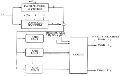
To complete the picture, a regular set of generalized residuals

CHAPTER 4. BDBUST OBSERVER-BASED FAULT DETECTION 37

is also designed. This time, simultaneous UIO’s with different functions of states are used. Given the g augmented systems, an UIO is designed to observe

different state functions of two or more systems. So more than one residual can be generated based on a single observer. Therefore, the number of observers deployed is reduced. The appeal to generating the residual set TZd in addition to the generalized set IZg is mainly to allow some sort of isolation in the case of multiple faults acting simultaneously. In fact, by partitioning the fault vector into smaller sets, the faults are squeezed into smaller groups and the isolation task is narrowed down to these groups. If the number of sets is high enough and/or well portioned, the redundancies allow an exact isolation of faults. Even if we fail to tell exactly which faults are affecting the system, we can at least limit them to a few possibilities. There is also the strategy of using these residuals in conjunction with some knowledge about the fault. For instance in the simulation example in the next chapter, the assumption that faults occur abruptly helps to exactly isolate them. Note that single faults are guaranteed to be detected and isolated thanks to TZg, in this case Rj, can be used for validation, to confirm the decision reached based on Rg.

Algorithm

There are two possible algorithms that can be followed in obtaining a simulta­ neous DDO for a given number of two or more systems. The first algorithm is based on Propositions 1.2, 2.1, and 2.2 and Theorem 2.1. The second is based on Theorems 2.2 and 2.3.

Given Ej, i = 1,2, of Section 3.1, the first algorithm that is used to design a functional simultaneous DDO is based on the fact that “either rank [Cl C2 Di D2] > rank [Di D2] or E has a stable invariant zero” is a necessary condition for its existence. The algorithm that is described in the

CHAPTER 4. ROBUST OBSERVER,-BASED FAULT DETECTION 39

‘if” part of Proposition 1.2 can hence be applied to the system matrix

Ai — s i 0 Bi 0 Sn{s) ■- = 0 A2 - S I 0 B2

Cl C2 Di D2

A lg o r ith m 1:

S tep 1: Determine if a constant matrix J exists such that J[Di D2] = 0 but Ti := JCi ^ 0 and T2 ;= JC2 0. If “yes” J is a constant simultaneous observer. If “no” check for a dynamic observer through steps 2-4.

S tep 2: Determine the Smith Normal Form (SNF) and the associated uni- modular matrices of <$'12(-5)· Let A ;= USuV, where U and V are unirnodular matrices, be the SNF.

S tep 3: Factorize A = A^A^ into stable-antistable matrices, with the stable matrix As square and nonsingular. Then, partition the stable rational and non­ polynomial matrix Aj^U = [ —X Y ] with X having 2n columns.

S tep 4: Write X = X+ -I- AT_, where AT_ is the strictly proper part of X. Expand the power series AT_ = X-iS~^ -I- X-i-iS~''~^ + ..., X^i 7^ 0 and I > 1.

S tep 5: Check if there exists a constant To such that TqX ^i =: [Ti T2]

(with each T having n columns) satisfies T / 0 for i = 1, 2. If “yes” , then The transfer function of a simultaneous DDO is Hy{s) = To(s^“ ^F)_. If a To exists further satisfying Ti = T2, then the constructed observer is a simultaneous DDO with the same state function.

The second algorithm can be applied if Ej, ¿ = 1,2, are both controllable. { s I - A i ) - ^ B i 0

Let 2^12(5) ~ 0 (si — A2)~^B2 _ Cl (si - AiY^Bi + Di C2(sl - A2)-^B2 + D2