HYBRID FOG-CLOUD BASED DATA
DISTRIBUTION FOR INTERNET OF
THINGS APPLICATIONS
a dissertation submitted to
the graduate school of engineering and science
of bilkent university
in partial fulfillment of the requirements for
the degree of
doctor of philosophy
in
computer engineering
By
Fırat Karata¸s
September 2019
HYBRID FOG-CLOUD BASED DATA DISTRIBUTION FOR IN-TERNET OF THINGS APPLICATIONS
By Fırat Karata¸s September 2019
We certify that we have read this dissertation and that in our opinion it is fully adequate, in scope and in quality, as a dissertation for the degree of Doctor of Philosophy. ˙Ibrahim K¨orpeo˘glu(Advisor) Ezhan Kara¸san ¨ Ozg¨ur Ulusoy Ahmet Co¸sar Ertan Onur
Approved for the Graduate School of Engineering and Science:
Ezhan Kara¸san
Copyright Information
Internal or personal use of this material is permitted.
c
Elsevier 2019. “With permission from F. Karatas and I. Korpeoglu, Fog-Based Data Distribution Service (F-DAD) for Internet of Things (IoT) applications, Fu-ture Generation Computer Systems, Volume 93, Pages 156-169, Elsevier, 2019”
ABSTRACT
HYBRID FOG-CLOUD BASED DATA DISTRIBUTION
FOR INTERNET OF THINGS APPLICATIONS
Fırat Karata¸s
Ph.D. in Computer Engineering Advisor: ˙Ibrahim K¨orpeo˘glu
September 2019
Technological advancements keep making machines, devices, and appliances faster, more capable, and more connected to each other. The network of all interconnected smart devices is called Internet of Things (IoT). It is envisioned that there will be billions of interconnected IoT devices producing and consuming petabytes of data that may be needed by multiple IoT applications. This brings challenges to store and process such a large amount of data in an efficient and effective way. Cloud computing and its extension to the network edge, fog com-puting, emerge as new technology alternatives to tackle some of these challenges in transporting, storing, and processing petabytes of IoT data in an efficient and effective manner.
In this thesis, we propose a geographically distributed hierarchical cloud and fog computing based IoT storage and processing architecture, and propose tech-niques for placing IoT data into its components, i.e., cloud and fog data centers. Data is considered in different types and each type of data may be needed by multiple applications. Considering this fact, we generate feasible and realistic network models for a large-scale distributed storage architecture, and propose al-gorithms for efficient and effective placement of data generated and consumed by large number of geographically distributed IoT nodes. Data used by multiple ap-plications is stored only once in a location that is easily accessed by apap-plications needing that type of data. We performed extensive simulation experiments to evaluate our proposal. The results show that our network architecture and place-ment techniques can be used to store IoT data efficiently while providing reduced latency for IoT applications without increasing network bandwidth consumed.
Keywords: Internet of Things, Fog Computing, Data Placement, Cloud Comput-ing, Network Topology, Data Management.
¨
OZET
NESNELER˙IN ˙INTERNET˙I UYGULAMALARI ˙IC
¸ ˙IN
H˙IBR˙IT S˙IS-BULUT TABANLI VER˙I DA ˘
GITIMI
Fırat Karata¸s
Bilgisayar M¨uhendisli˘gi, Doktora Tez Danı¸smanı: ˙Ibrahim K¨orpeo˘glu
Eyl¨ul 2019
Teknolojik geli¸smeler makineleri, e¸syaları ve cihazları daha hızlı, daha yetenekli ve birbirleriyle daha ba˘glı hale getirmeye devam etmektedir. Birbirlerine ba˘glı bu akıllı cihazların olu¸sturdu˘gu a˘g yapısı Nesnelerin ˙Interneti (IoT) olarak ad-landırılmaktadır. Bu milyarlarca cihazın, birden fazla IoT uygulamasının ihtiya¸c duydu˘gu ve duyabilece˘gi petabaytlarca veriyi ¨uretme ve/veya kullanma yetenek-lerine sahip olaca˘gı ¨ong¨or¨ulmektedir. Bu durum, b¨uy¨uk miktardaki bu verinin etkin ve verimli bir ¸sekilde depolanması ve i¸slenmesi gibi zorlukları da beraberinde getirmektedir. Bulut bili¸sim ve onun son kullanıcılara yakınla¸stırılmı¸s versiy-onu olan sis bili¸sim, IoT verilerinin verimli ve etkili bir ¸sekilde nasıl ta¸sınaca˘gı, yerle¸stirilece˘gi, saklanaca˘gı ve i¸slenece˘gi ile ilgili bu zorlukların bazılarının ¨
ustesinden gelebilmek i¸cin yeni y¨ontemler ortaya koymaktadır.
Bu tezde; co˘grafi olarak da˘gıtık, hiyerar¸sik bulut ve sis bile¸senlerini i¸ceren bir IoT mimarisi ve olu¸sturulan b¨uy¨uk miktardaki IoT verisinin bu mimarinin bile¸senlerine, bulut ve sis veri merkezlerine, yerle¸stirmek i¸cin yeni teknikler ¨
oneriyoruz. Verilerin sınıflandırılabilece˘gi g¨oz ¨on¨unde bulunduruldu˘gunda, bir-den fazla uygulama bu verileri kullanabilir. Bu bilgiye dayanarak, co˘grafi olarak da˘gıtık IoT cihazlarının olu¸sturdu˘gu ve kullandı˘gı verileri, ger¸ceklenebilir a˘g mod-ellerinde etkin ve verimli ¸sekilde veri merkezlerine yerle¸stirecek algoritmalar tasar-layıp, bunları tamsayı do˘grusal modelleme y¨ontemi kullanılarak elde edilen op-timum sonu¸clarla kar¸sıla¸stırıyoruz. Birden fazla uygulama tarafından kullanılan verileri, kopyalamadan ve o veriyi kullanan b¨ut¨un uygulamalar tarafından ra-hatlıkla eri¸silebilecek bir merkezde saklıyoruz. ¨Onerdi˘gimiz a˘g mimarisi ve algo-ritmalar sayesinde; verilerin etkin ve verimli ¸sekilde yerle¸stirilebilece˘gini, uygula-maların bu verilere bant geni¸sli˘gini arttırmadan daha hızlı ¸sekilde eri¸sebilmesine olanak sa˘gladı˘gını yaptı˘gımız kapsamlı sim¨ulasyon deneylerinin sonu¸clarıyla do˘gruluyoruz.
vi
Acknowledgement
I would like to express my sincere gratitude to my advisor Prof. ˙Ibrahim K¨orpeo˘glu for his guidance and patience. I am grateful for his encouragement and support during my hard times throughout the study, and I really appreciate that.
I would like to thank the members of the thesis monitoring committee, Prof. Ezhan Kara¸san and Prof. ¨Ozg¨ur Ulusoy for their precious comments and ideas during this long journey. I would also like to thank my thesis defense jury Prof. Ahmet Co¸sar and Assoc. Prof. Ertan Onur for accepting the invitation and taking a part in my defense jury.
I want to express my deepest gratitude to my family. Without their encourage-ment and patience I would not be here. I always sense their unlimited love and support in my heart. I also apologize from them for missing irreversible moments during this study.
I am very grateful to Prof. ˙Ibrahim Barı¸sta from Medical Oncology Depart-ment of Hacettepe University during my hard times. I cannot accomplish this without him and my family.
I also want to thank my beloved friends who are always with me every time. I would especially thank Cem Mergenci for organizing the thesis monitoring com-mittees together.
I am thankful to my supervisors and colleagues in Meteksan Defence Ind. Inc. for their support and encouragement.
The financial support of the Scientific and Technological Research Council of Turkey (TUB˙ITAK) through the B˙IDEB 2211 program is appreciated.
Contents
1 Introduction 1 1.1 Thesis Outline . . . 5 2 Related Work 7 2.1 Network Architecture . . . 7 2.2 Resource Allocation . . . 8 2.3 Data Placement . . . 103 Proposed Hybrid Fog-Cloud Based IoT Data Placement System Architecture 12 3.1 Hybrid Fog-Cloud Based Network Architecture . . . 13
3.2 Data-Centric IoT Data Placement Strategy . . . 14
3.3 Data Classifier and Data Profiler Agents . . . 15
3.4 Summary . . . 18
4 IoT Data Placement Problem in Hybrid Fog-Cloud Based Ar-chitecture 19 4.1 Analytical Model of Data Placement in Hybrid Fog-Cloud Archi-tecture . . . 20
4.2 Relation Between Applications and Data Usage . . . 27
4.3 Proof of the Linearity of Mathematical Model . . . 31
4.4 Summary . . . 34
5 Algorithms for Data Placement Problem in Hybrid Fog-Cloud Based Architecture 36 5.1 Algorithm 1 . . . 37
CONTENTS ix
5.2 Algorithm 2 . . . 39
5.3 Algorithm 3 . . . 41
5.4 Algorithm 4 . . . 44
5.5 Summary . . . 47
6 Hybrid Fog-Cloud Computing Based Network Topology Model-ing 48 6.1 Hybrid Network Topology Modeling Algorithm . . . 49
6.1.1 Rectangular Area Creation . . . 50
6.1.2 Placement of CCs and Assigning FCUs . . . 56
6.2 Length, Area and Cluster Relations . . . 64
6.2.1 Length Distributions . . . 64
6.2.2 Area Relationship of Rectangles . . . 67
6.2.3 Cluster Relationship . . . 70 6.3 Summary . . . 72 7 Performance Evaluation 73 7.1 Simulation Parameters . . . 74 7.2 Algorithms Used . . . 76 7.3 Latency Results . . . 78
7.3.1 Effect of Applications Run Ratio on Latency . . . 78
7.3.2 Effect of Excess Use on Latency . . . 86
7.4 Storage Results . . . 91
7.4.1 Effect of Applications Run Ratio on Data Storage . . . 92
7.4.2 Effect of Excess Use on Data Storage . . . 95
7.4.3 Effect of Storage Capacities on Data Storage . . . 99
7.5 Algorithm Run-Time Results . . . 102
7.6 Network Occupancy Results . . . 103
7.7 Summary . . . 105
List of Figures
3.1 An example FCU consisting of 2 FCs and 10 IoT nodes. . . 14
3.2 Example scenarios of Data Classifier & Data Profiler agents in the proposed architecture. . . 17
4.1 An example of application - data type relation graph. . . 28
4.2 An example of network & data dependency graph (2 FCUs, 1 CC, 5 applications and 3 data types). . . 33
6.1 Examples of vertical and horizontal rectangle cuts. . . 51
6.2 Horizontal & vertical cut flowchart. . . 52
6.3 An example of vertical cuts over horizontal ones. . . 52
6.4 An example of a rectangle generated by the algorithm. . . 55
6.5 Examples of undivided/divided circumscribed circles. . . 57
6.6 Cluster centers in the first iteration of k-means algorithm. . . 57
6.7 An example of k-means choosing nearest CC. . . 59
6.8 An example of k-means choosing less crowded CC. . . 59
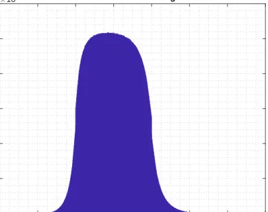
6.9 Histogram of all lengths in 10 million sample division. . . 65
6.10 Histograms of Length # 1 to # 6. . . 66
6.11 Histograms of Length # 7 to # 10. . . 67
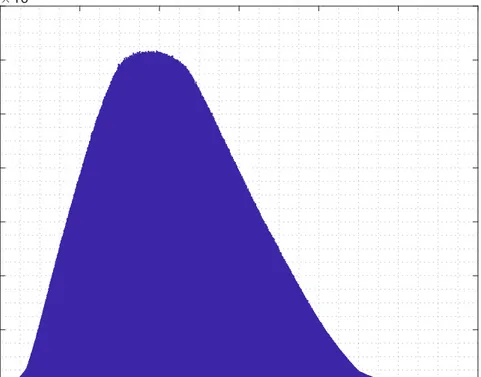
6.12 Histogram of all areas in 10 million sample division. . . 68
6.13 Histograms of Areas # 1 to # 6. . . 69
6.14 Histograms of cluster areas and node counts according k-means strategies. . . 71
LIST OF FIGURES xi
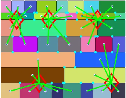
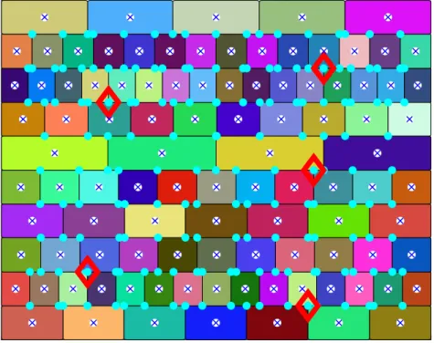
7.1 Smart city example network: M = 5, N = 100. Blue crosses are FCU centers and cyan points are possible CC locations. After using k-means with less crowded CC strategy chosen CC places
are marked with red diamond. . . 75
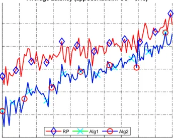
7.2 Average latency (EU = 10, appUseRatioInFCU = 0.05). . . 79
7.3 Average latency (EU = 10, appUseRatioInFCU = 0.1). . . 79
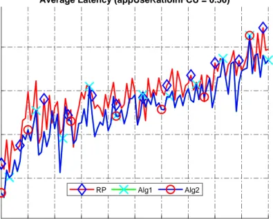
7.4 Average latency (EU = 10, appUseRatioInFCU = 0.5). . . 80
7.5 Average latency (EU = 10, appUseRatioInFCU = 0.75). . . 80
7.6 Average latency (EU = 10, appUseRatioInFCU = 1.0). . . 81
7.7 Average latency (EU = 10, appUseRatioInFCU = 0.05). . . 82
7.8 Average latency (EU = 10, appUseRatioInFCU = 0.1). . . 82
7.9 Average latency (EU = 10, appUseRatioInFCU = 0.5). . . 83
7.10 Average latency (EU = 10, appUseRatioInFCU = 0.75). . . 83
7.11 Average latency (EU = 10, appUseRatioInFCU = 1.0). . . 84
7.12 Average latency (EU = 10, appUseRatioInFCU = 1.0). . . 85
7.13 Average latency (EU = 10, appUseRatioInFCU = 1.0). . . 86
7.14 Average latency (appUseRatioInFCU = 0.2, EU = 2.5). . . 87
7.15 Average latency (appUseRatioInFCU = 0.2, EU = 5.0). . . 87
7.16 Average latency (appUseRatioInFCU = 0.2, EU = 10.0). . . 88
7.17 Average latency (appUseRatioInFCU = 0.2, EU = 2.5). . . 89
7.18 Average latency (appUseRatioInFCU = 0.2, EU = 5.0). . . 89
7.19 Average latency (appUseRatioInFCU = 0.2, EU = 10.0). . . 90
7.20 Total used CC & FCU storage capacities (appUseRatioInFCU = 0.2, EU = 5.0). . . 93
7.21 Total used CC & FCU storage capacities (appUseRatioInFCU = 0.5, EU = 5.0). . . 94
7.22 Total used CC & FCU storage capacities (appUseRatioInFCU = 1.0, EU = 5.0). . . 95
7.23 Total used CC & FCU storage capacities (appUseRatioInFCU = 0.05, EU = 10.0). . . 96
7.24 Total used CC & FCU storage capacities (appUseRatioInFCU = 0.05, EU = 20.0). . . 97
LIST OF FIGURES xii
7.25 Total used CC & FCU storage capacities (appUseRatioInFCU = 0.05, EU = 30.0). . . 98 7.26 Total used CC & FCU storage capacities (Average capacity in an
FCU = 5GB). . . 99 7.27 Total used CC & FCU storage capacities (Average capacity in an
FCU = 7GB). . . 100 7.28 Total used CC & FCU storage capacities (Average capacity in an
FCU = 15GB). . . 101 7.29 CPU run times of algorithms (appUseRatioInFCU = 1.00, EU =
10.0). . . 102 7.30 Network occupancy (appUseRatioInFCU = 0.1, EU = 30). . . 104 7.31 Network occupancy (appUseRatioInFCU = 0.1, EU = 30). . . 104
List of Tables
4.1 Notations of problem formulation. . . 23
6.1 Mean and variances of generated lengths. . . 65
6.2 Mean and variances of generated areas. . . 68
6.3 Mean and variances of cluster areas and node counts. . . 70
Chapter 1
Introduction
The idea of enabling communication between any pair of devices has led to the emergence of Internet of Things (IoT), which encompasses all techniques and technologies to interconnect all kinds of devices with each other via the Internet. This evolution has started first with the design of radio frequency identifiers (RFIDs) for small devices and things by using RFID technology and monitoring the states of tagged devices, and then continued with the developments in wireless sensor networks (WSN) [1].
There is an extensive amount of research and development going on in the IoT field [2]. As the types and the number of nodes constituting IoT are increasing ev-ery day, new and interesting IoT applications are envisioned and built [3] as well. Not only the applications, but also the different types of technologies depending on IoT are increasing. There are a lot of studies explaining the evolution in IoT applications and technologies with future trends and research challenges [4–8].
Advances in IoT and development of new IoT products enable new kinds of IoT concepts. For example, the advances make wearable smart devices connected to the Internet popular, and now they are named as Wearable IoT (WIoT) [9]. Also, it is expected in the near future that the concept of smart cities [10] will be implemented and deployed, and there are a lot of research activities going on to
tackle the related challenges [11–13].
While IoT technologies were evolving, new communication and networking technologies supporting IoT have been designed as well. One of these is the low-power wide area networks (LPWAN) technology [14, 15], which is a long-range low-rate wireless communication technology that consumes low power. With up-coming communication technologies, releasing the potential of IoT will become faster. For example, 5G technology will increase the communication speed and coverage between devices to support high-rate and high-quality demanding ap-plications [16].
Various applications can use IoT technology nowadays. Some of these applica-tions include, but not limited to, crowd-sensing [17], smart home [18] and smart grid [19]. Since the number of potential applications is growing steadily, a classi-fication can help to see the trends and analyze the requirements, and Scully [20] does this by classifying all IoT applications into ten different groups. These ap-plications are reviewed and explained in various papers, such as [21–23], and one of the common problems of these applications is handling big data.
Since the number nodes forming IoT can increase exponentially, the volume of data generated and consumed by these nodes can increase to an unprece-dented level [24]. Storing and processing such a big volume of data is a daunting task [25]. This becomes especially challenging when IoT nodes are geographically distributed to a very large region [26].
Distributed cloud computing technology is an attractive alternative to store and process large volumes of data [27]. Cloud computing can be used to as-sign complicated and resource hungry tasks to capable data centers distributed around the world [28]. New architectures are needed, however, to integrate cloud computing with IoT [29]. Cisco is one of the first companies suggesting the idea of edge and fog computing that extends the cloud computing capabilities closer to the places where data is generated and consumed [30]. In this architecture, besides large cloud computing data centers, there are a lot of smaller data centers distributed in the region of interest providing fog computing capabilities, storing
and processing data in the field.
Fog computing data centers are small projections of more capable cloud data centers. Applications, research challenges and other issues related to fog comput-ing are reviewed in various articles [31–34].
Integration of cloud and fog computing paradigms together with IoT requires the adaptation of the applications to this approach. One problem to consider is how to place and use application data in the components of the distributed and centralized cloud infrastructure [35,36]. Such an infrastructure will enable a lot of new data-intensive applications, and these applications may share the generated IoT data. The dependency relationship of the applications to the data becomes critical in designing data placement strategies.
In this thesis, we focus on this problem of designing a cloud and fog based IoT data storage architecture and related data placement methods on this in-frastructure. We first propose a hybrid hierarchical architecture consisting of geographically distributed cloud and fog computing data centers to extend the capabilities of IoT devices, and to store and process large volumes of IoT data. Leaves of the hybrid architecture are IoT devices and they are the least capable components available in the architecture. Primary services offered by the cloud and fog data centers in the proposed architecture is data-as-a-service (DaaS) [29], which may enable commercially valuable data-driven IoT applications in a cost-efficient manner.
With data-as-a-service, a network consisting of IoT nodes with both cloud and fog computing data centers can create a data market [37]. In such data market, there are data generators, consumers, and marketplaces. Data is provided to the market by various types of sensors, which are less capable IoT nodes, and applications running in smarter IoT nodes consume the generated data. Fog and cloud computing data centers are the marketplaces where data storages and exchanges occur. Therefore, IoT nodes can be considered as data generators, data consumers or both, and data centers are the places where data resides.
We propose the IoT nodes in a certain local region to be considered together with the fog data center(s) near them to constitute an architectural element called Fog Computing Unit (FCU). These units are built by the combination of heterogeneous IoT nodes and one or more fog computing data center(s). In each unit, capabilities of all elements can be shared among others.
A lot of customers, i.e., applications, may share common demand for data and this may become an important optimization factor, since the amount of data shared by applications may be quite large. If each application stores the needed data separately to maximize its benefits, which we name as application-centric approach, storing and handling such a large amount of data can become very costly and inefficient. This raises the question of how to handle huge amount of data efficiently without disrupting application requirements.
To overcome the inefficient data storage problem, we propose that data gener-ated by IoT nodes to be considered in types and each type of data to be stored only in one location which is optimum for multiple applications requiring it. We call this approach as data-centric approach. Based on this approach, we pro-pose methods about where to store different types of data efficiently so that the applications can reach their required data with the lowest feasible latency.
Part of this thesis is based on our work in [38], which is proposing consideration of IoT data in different types, and at the same time proposing methods to place different types of data efficiently and effectively into fog and cloud data centers. While considering the needs of geographically distributed IoT nodes, we also consider how to decrease the storage costs without affecting the performance, which is important from the DaaS providers point of view.
Since there is no known deployed or well-known verification environment to test fog based IoT algorithms, we also developed a model for hybrid fog-cloud based IoT networks. By using this model we tested our heuristic algorithms.
1. We propose a hybrid hierarchical fog-cloud computing data center network architecture involving IoT nodes for storing and processing IoT data effi-ciently.
2. We propose the consideration of IoT data in various and well-defined types, based on the consideration that multiple IoT application may need to access the same data. This allows efficient data storage, since data can be stored only in one place and can be shared. While doing this, we also care about not increasing network overhead and satisfying delay requirements.
3. According to the proposed data classification architectural model, we de-velop a mathematical model for average data access latency that applica-tions encounter, and provide an integer programming solution.
4. To achieve the best performance according to the given analytical model without using linear solvers, we propose efficient data placement heuristic algorithms to place the data in the mesh network of fog computing units, which can provide efficient storage, low latency and reduced network over-head compared to application-centric approach.
5. Since there is no known deployed fog-cloud based IoT architecture, we pro-pose a method to model hybrid fog-cloud computing networks, and use this model for the evaluation of our data placement algorithms.
1.1
Thesis Outline
The rest of this thesis is organized as follows. In Chapter 2, we give the state-of-the-art and related work in IoT and handling of IoT data. In Chapter 3, we specify the IoT data placement problem and propose a hybrid and hierarchical fog-cloud based IoT storage architecture. In Chapter 4, we explain our analytical model and give linear programming solution for the data placement problem in the proposed storage architecture. In Chapter 5, we propose heuristic data placement algorithms that can be used in the proposed architecture when the network of fog and cloud data centers gets larger. In Chapter 6, we explain the
methods and our model for the simulated IoT network, which is required for the evaluation of the algorithms. In Chapter 7, we present the results of our extensive simulation experiments done based on the proposed IoT network model. Finally, we give our conclusions and future work in Chapter 8.
Chapter 2
Related Work
Fog computing, an extension of cloud computing, tries to push clouds through edges of the network, and can be employed in IoT networks to store and process IoT data more effectively and efficiently. All of the work done in the literature related to cloud and fog computing together with IoT have significant importance to this research. On top of these studies, we focus on an important challenge of big data placement in networks consisting of these elements where some of them have limited resources (especially in IoT nodes). Under the light of these, we can group fog-cloud enabled IoT related research studies into three major groups:
1. Network architecture and use cases. 2. Allocation of available resources. 3. Data placement strategies.
2.1
Network Architecture
The first group of related work consists of architectural and theoretical work done in cloud and fog enabled IoT. In one of these works, Bonomi et al. [26] explain the
interplay of data in combination with IoT and fog-cloud computing paradigms, and give some architectural structures for applications running in IoT nodes.
Since deploying and designing a smart city from network perspective is chal-lenging and competitive; verifying the algorithms and use cases of the smart city requires effort. For making these easier Santos et al. define a framework and testbed called City of Things (CoT) [39] and deploy it in Antwerp, which enables researchers to test possible IoT applications in smart cities. In another work, Zanella et al. [21] describe a proof-of-concept system architecture for a smart city application which is deployed in Padova.
Architectural designs vary according to use cases, and Santos et al. [40] explain a hypothetical network structure for smart city applications using the 5G net-work. Most of the network architectures enabling fog computing concept require intelligent gateways and routers in the edges. As an example of these, including, but not limited to, Aazam and Huh explain the smart gateway concept in [41], and Jutila gives an efficient edge router in [42].
2.2
Resource Allocation
The second group of related work is resource provisioning or allocation, which is inevitable where resources are limited and lots of demanders such as customers, users, applications, etc., need to use them. Proper resource allocation is one of the most important problems not only in cloud and fog computing but also in IoT where the capabilities of nodes are limited, and therefore resources should be used efficiently by applications and users. There is a lot of work done on resource provisioning in cloud computing data centers and examples of this research are including, but not limited to [43–46].
An important resource in IoT nodes that needs to be used carefully is the network bandwidth, which is usually shared by a lot of applications. Angelakis et al. [47] propose an allocation model for heterogeneous resource demands by
considering activation and utilization metrics of available network interfaces in IoT devices. Tsai [48] proposes a network resource allocation algorithm for IoT devices, called SEIRA, based on search economics for exploring solution space for getting close to the optimum. Lera et al. [49] consider reducing network usage by placing IoT data on fog computing nodes according to centrality indices. However, they do not consider the characteristics of the distributed applications running in the network, such as their quality-of-service requirements, data access patterns, or where they are running.
In another group of the resource allocation studies, researchers want to answer how IoT modules should be decoupled into fog and cloud computing nodes such that the quality-of-service requirements are met. In one of these works, Taneja and Davy consider partitioned application module layers and aim to place each of these modules to computing nodes efficiently [50]. In another work, Rezazadeh et al. [51] try to place IoT modules in fog and cloud nodes using simulated anneal-ing. The same group propose a heuristic called LAMP to decrease the latency applications encounter by placing different IoT application modules to fog and cloud computing nodes [52]. Natesha and Guddeti use another heuristic called First-Fit Decreasing (FFD) aiming again to decrease the latency applications encounter together with the power consumption of computing nodes [53].
Resource provisioning is also another very important problem in more limited fog computing data centers. Tocze and Nadjm-Tehrani [54] classify resources in fog computing and survey the related research works and issues based on their taxonomy. In their work, they discuss that data and storage mechanisms are not well-studied in the literature. Another important shared resource in fog data centers is computational components, and their utilization is considered in some workload allocation studies. Deng et al. [55] model a hybrid fog-cloud com-puting architecture by dividing the network into four subsystems and propose a mathematical framework for optimizing workload sharing mechanism among data centers while considering power consumption and delay. Tong et al. [56] present a workload allocation strategy for mobile computing nodes by pushing cloud data centers to the edges hierarchically and naming them as hierarchical edge cloud. They try to allocate available computational resources on data centers used by
mobile workloads efficiently. Besides computational resources, I/O interfaces and resources are also limited in fog computing nodes, and Zeng et al. [57] consider these in a fog computing enabled embedded system.
There are also studies focusing not only on one specific type of resource but also considering the general concept of resource sharing in fog computing. Arkian et al. [58] describe MIST, which is a less dense communication scheme for fog computing, and model the resource provisioning problem with a mixed-integer nonlinear programming (MINLP) model by considering limited capabilities of fog nodes in mobile crowd-sensing applications. They mainly focus on a specific application and the reduction of their nonlinear MIST model to a linear one. Skarlat et al. [59] discuss a software-based resource allocation scheme in fog en-abled IoT environments with the help of fog colonies. They try to distribute task requests or data among these colonies by using an entity called fog cell. Al-though fog colonies resemble fog computing units, they do not include IoT nodes and their work does not consider data and applications independently. Yu et al. [60] tackle resource sharing problem mainly focusing on applications. They investigate real-time application provisioning in a fog enabled IoT network with the aim of satisfying applications’ quality-of-service (QoS) requirements such as bandwidth and delay. Although they consider latency encountered by applica-tions in their work, they do not focus on where data resides or how it is placed.
2.3
Data Placement
The third group of related work is data placement strategies. Qin et al. [61] dis-cuss the differences between data characteristics of IoT and traditional Internet applications while focusing on the data taxonomy in IoT. They emphasize that in the conventional Internet, data is mainly generated by human beings, but it is generated and consumed by IoT devices. Since it is easy to distribute these smart and interconnected devices all around the world, data can be generated and consumed by geographically distributed nodes, and as the number of smart devices increase, data placement for these devices becomes an important issue.
Problems relevant to fog computing are also valid in other more mature domains such as Online Social Networks (OSN) where the users are geographically dis-tributed as well. Yu and Pan [62] handle data placement problem in OSNs by using hypergraph partitioning techniques in geographically distributed data cen-ters and nodes. In their work, they do not consider the capacity limitations of data centers, which is crucial in fog computing enabled IoT networks. Tang et al. [63] discuss the advantages of the geographical distribution of fog computing nodes in smart cities for handling the big data generated by IoT nodes in various use cases.
Various other researchers also consider data-centric use cases and placement. Oteafy and Hassanein [64] discuss the importance and advantages of data-centric placement in fog enabled IoT architectures for reducing access latencies, and envision that applications requiring low latency can proliferate. An example of these applications is streaming based traffic monitoring [65]. Publish-subscribe models are also investigated and one model for DaaS on clouds has been proposed in IoT architectures by defining a quality of data metric, which relies on extracting useful and required data in smart city applications [66].
Chapter 3
Proposed Hybrid Fog-Cloud
Based IoT Data Placement
System Architecture
We focus on networks which are composed of cloud and fog computing data cen-ters together with the geographically distributed and less capable IoT nodes. By grouping and using these incapable nodes in each group with harmony, complex applications may run and each of these may need some sort of data produced by other nodes or groups. As the number of these less capable nodes increase, processing, distributing and storing data become problematic. Therefore, we try to answer the question of how to distribute and store data required by the geographically distributed nodes in this section.
In this chapter, we start with defining our hierarchical hybrid fog-cloud based network architecture (Chapter 3.1) which consists of both fog and cloud data cen-ters together with less capable IoT nodes for overcoming distribution and storage problems. On top of the considered network architecture, we explain a place-ment strategy which we call data-centric approach (Chapter 3.2). And finally, we present agents which are called Data Profiler and Data Classifier needed for this solution to work in the defined network efficiently (Chapter 3.3).
3.1
Hybrid Fog-Cloud Based Network
Architec-ture
The network architecture starts with considering the hierarchical structure of geo-distributed IoT data that is mentioned in the work of Bonomi et al. [26]. In their geo-distributed structure, latency increases as data goes from IoT nodes to cloud computing centers and this creates a problem for applications requiring low latencies. A lot of IoT applications are inherently geo-distributed, like smart-city applications, and therefore increased latency in such a geo-distributed system is inevitable if proper precautions are not applied. Bearing these in mind, we propose a hierarchical system and network architecture consisting of IoT nodes and cloud computing data centers, and fog computing centers in between. This is similar to the neighborhood concept in smart cities which includes fast responsive edge computing nodes connected to IoT nodes [63]. In our proposed architecture, we replace the edge nodes by (F)og (C)omputing data centers (FC), which are small projections of cloud data centers and located near to the field. IoT nodes in a region are connected to a fog computing data center located near them and together they form a storage and processing unit called (F)og (C)omputing (U)nit (FCU). The remaining building block of the architecture is (C)loud (C)omputing data centers (CC), as usual, and they are possible candidates for storing and serving data together with fog computing nodes. If the available resources of fog computing data centers are not enough for storing data, the cloud data centers are the ultimate places to store data.
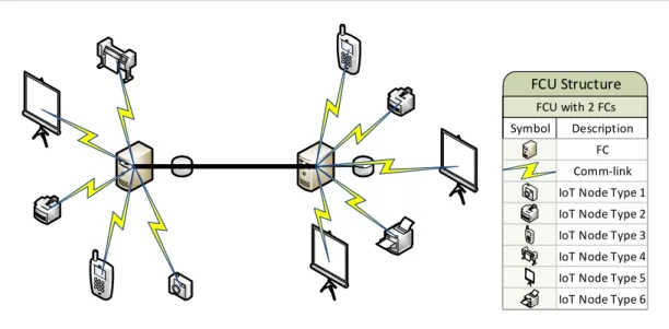
A large volume of data is generated and consumed by IoT nodes. IoT nodes in a region send and receive data to/from their directly connected FC nodes. In an FCU, IoT nodes and the FC node(s) are connected with star topology (see Figure 3.1). There may be more than one FC in an FCU. All FCUs and CCs are connected via a mesh logical topology. The main difference between FCUs and CCs is the availability of resources. Since FCs are small projections of CCs and IoT nodes have restricted capabilities, available resources in FCUs are limited, but in CCs resources are assumed as unlimited.
Symbol Description FCU with 2 FCs FCU Structure
IoT Node Type 1 FC Comm-link
IoT Node Type 2 IoT Node Type 3 IoT Node Type 4 IoT Node Type 5 IoT Node Type 6 Symbol Description
FCU with 2 FCs FCU Structure
IoT Node Type 1 FC Comm-link
IoT Node Type 2 IoT Node Type 3 IoT Node Type 4 IoT Node Type 5 IoT Node Type 6
Figure 3.1: An example FCU consisting of 2 FCs and 10 IoT nodes.
3.2
Data-Centric IoT Data Placement Strategy
In Section 3.1, we define the network architecture which only shows the possible places of data, in this section we want to explain the data placement problem and present a solution strategy. The big data generated for possible consump-tion needs to be first stored in the network efficiently and effectively. It can either be stored regionally in the FCUs or the corresponding CCs. Since a lot of applications may need the same type of data, we can develop clever place-ment approaches and algorithms for storing data. Instead of storing the needed data for each application separately, it is possible to store it once and distribute it among all IoT applications in need. This requires first the categorization of data. We propose the generated data to be partitioned, i.e., classified into several well-defined types and all data of some certain type to be stored only once and shared by all interested applications. Also, some applications may require several different types of data for doing their jobs correctly. In this case, they access all the required data of different types from the locations where they reside. We call this as data-centric approach for placing, storing and using data by multiple ap-plications. We call the other approach where data of some certain type is stored separately for each interested application as application-centric data placement. Data is not shared in the application-centric approach.
As a motivational example, consider an accident between a car and a pedestrian in a smart city. Smart poles observing the accident can generate health data of the pedestrian and can monitor the traffic nearby. Connected cars in the city can also generate information about the traffic. Let another case be an emergency situation related to a resident in one of the smart homes which is also happening almost at the same time as the traffic accident. Sensors in the home generate vital data of the patient and send it to health services for an emergency rescue. By gathering both health and traffic data, the emergency services can easily optimize available resources, which are ambulances in these cases, and give the task of reaching emergency incident places with the ambulances in the fastest way. In the example, traffic and health data are two different types of data generated by IoT nodes distributed all over the city. Assigning and routing ambulances for two distinct incidents as fast as possible is an application requiring these two different types of data. Now, consider the navigation application which is popular and commonly used in a smart city as another application running. It also requires traffic data as in the case of health services and if the application-centric data placement is used, the traffic data will be duplicated. By using the data-centric approach and classifying data into types and placing them accordingly, we avoid the unnecessary replication of data and reduce the storage costs accordingly.
3.3
Data Classifier and Data Profiler Agents
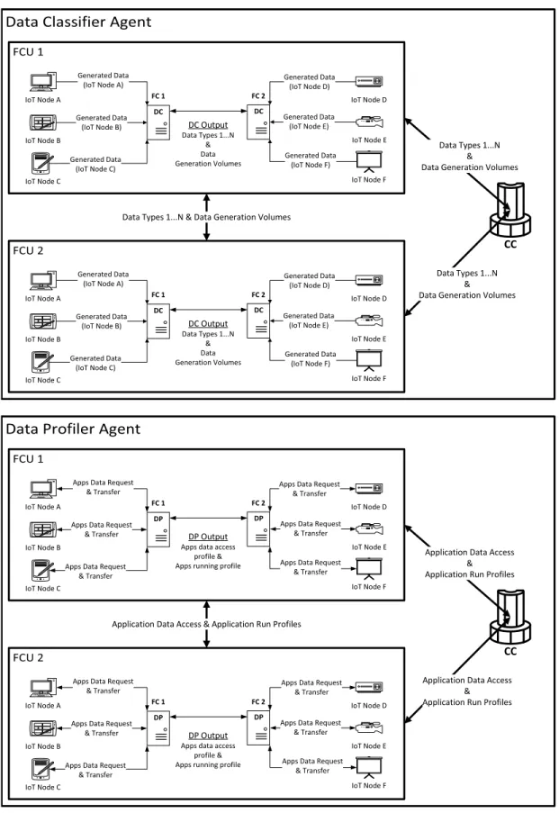
The data-centric approach requires decoupling of data from applications. Using the structural elements defined in [67] with intelligent classification agents running in them, enable the decoupling of data from applications, and make data-centric placement approach possible. IoT nodes are connected to an FC and they are the sources of generated data. An agent process, called (D)ata (C)lassifier (DC), running in all FCs can be used to classify data generated in the network. DC can also monitor the data generation volumes of each data type in each FCU during the classification process. IoT nodes are the places where applications run and consume data, so their access characteristics to data and their running frequencies need to be profiled for intelligent data placement as well. Another
agent called (D)ata (P)rofiler (DP) works as profiling mechanism of applications. DC and DP agents together can measure and derive the data characteristics of IoT nodes, and notify the central mechanism for data placement procedures (see Figure 3.2). Since IoT nodes are elements of FCUs, outputs of DC and DP agents running in FCs give an idea about the data generation and usage characteristics in FCUs. According to the outcome of the agents, data placement decisions can be done adaptively.
An important benefit of classifying data and storing it once for each class is added flexibility for designing new applications without considering the data needs. Designers can use a publish-subscribe mechanism for accessing the avail-able data types in the network. From data management perspective, duplication is not needed in the case where data is used by more than one application and this enables the reduction of storage costs. Regarding that point of view, the data-centric approach can perform better than the application-data-centric data placement approach dramatically.
Decreasing the storage costs by using the data-centric approach is an important benefit. However, latencies encountered by applications have to be kept in mind as well. We can achieve this by placing required data to the geographically close places where interested applications run. The issue here is that more than one application may want to use the data of the same type and these applications can be at distinct and far away locations. Another assumption in the architecture is that each application running in IoT nodes need to access a small amount of data (compared to whole data stored) in the interaction time. Therefore, propagation delay in accessing the needed data of certain type dominates the response time. Effect of the processing delay is negligible. 1 With the help of
1The reason is although optical fiber connections are used, a request has to be made from
the demanding node and it is transmitted at the speed of light. A small response message is transmitted back to the requested node from the destination which also travels at the speed of light. So the propagation delay becomes “(2 × Distance) / Speed of light”, and it is roughly 0.4msec for a 60km distance. If small amount of data is assumed to be 1KB, then its processing time becomes in the order of nanoseconds when a simple RAID 0 architecture used with two SSDs whose read speeds are 500MB/s with SATA III interface. In today’s data centers, much faster SSDs with PCI-Express interfaces can be used and this also reduces the processing times significantly since their read/write speeds are in the order of GB/s.
CC IoT Node D IoT Node E IoT Node F Generated Data (IoT Node D) Generated Data (IoT Node E) Generated Data (IoT Node F) FC 1 IoT Node A IoT Node B IoT Node C Generated Data (IoT Node A) Generated Data (IoT Node B) Generated Data (IoT Node C) DC DC Output Data Types 1...N & Data Generation Volumes Data Types 1...N &
Data Generation Volumes
Data Types 1...N & Data Generation Volumes
Data Types 1...N &
Data Generation Volumes
FC 2 DC IoT Node D IoT Node E IoT Node F Generated Data (IoT Node D) Generated Data (IoT Node E) Generated Data (IoT Node F) FC 1 IoT Node A IoT Node B IoT Node C Generated Data (IoT Node A) Generated Data (IoT Node B) Generated Data (IoT Node C) DC DC Output Data Types 1...N & Data Generation Volumes FC 2 DC CC IoT Node D IoT Node E IoT Node F Apps Data Request
& Transfer
Apps Data Request & Transfer
Apps Data Request & Transfer
FC 1
IoT Node A
IoT Node B
IoT Node C
Apps Data Request & Transfer
Apps Data Request & Transfer
Apps Data Request & Transfer
DP
DP Output Apps data access
profile & Apps running profile
Application Data Access & Application Run Profiles
Application Data Access & Application Run Profiles
Application Data Access & Application Run Profiles
FC 2 DP
IoT Node D
IoT Node E
IoT Node F Apps Data Request
& Transfer
Apps Data Request & Transfer
Apps Data Request & Transfer
FC 1
IoT Node A
IoT Node B
IoT Node C
Apps Data Request & Transfer
Apps Data Request & Transfer
Apps Data Request & Transfer
DP
DP Output Apps data access
profile & Apps running profile
FC 2 DP
Figure 3.2: Example scenarios of Data Classifier & Data Profiler agents in the proposed architecture.
DP, running frequencies of applications can be compared and for reducing the average latency encountered, the shared data type can be placed near to the application which runs and accesses it more. This reduces data placement to an optimization problem where the average data access latency of applications running in the geographically distributed FCUs needs to be minimized without duplicating the data. We formulate this optimization problem and give its linear model in Chapter 4.
Under the scope of our model, the mobility of applications or fast changes that affect the outcomes of DC and DP agents are not considered. Our placement model assumes that all outcomes of agents are available and placement decisions are made accordingly. If significant changes are detected in the outcomes of the agents, placement algorithms have to be rerun.
3.4
Summary
In this chapter, we start with explaining a network model consisting of cloud computing data centers, IoT nodes and fog computing data centers in between. We merge the geographically close fog computing data centers and IoT nodes, and name each of these merged groups as fog computing unit (FCU).
By using the available storage resources of FCUs with harmony, we want to decrease storage burden on cloud computing data centers. For doing it so, we need to split data into well-known types and store in types. We call it as the data-centric placement approach.
Finally, we describe two agents required to make data-centric placement ap-proach feasible. One of the agents is responsible for splitting data and we name it data classifier (DC), and the second agent is responsible for monitoring the data access and running characteristics of the applications in FCUs.
Chapter 4
IoT Data Placement Problem in
Hybrid Fog-Cloud Based
Architecture
In the previous chapter, we explain a structural solution for data placement prob-lem, and in this chapter we present the analytical model of the problem. As mentioned at the end of Section 3.3, when multiple applications and data types exist in network, data placement turns into a problematic task. By using the outputs of agents defined, we can reduce it to an optimization problem and give the solution in Section 4.1. According to the optimization model we define any of the commercial linear solvers such as Gurobi [68] or CPLEX [69] can give the optimum solution of the problem.
One of the important obstacles for developing new IoT applications is the data to be used. Since we consider data in well-defined types, new applications can be developed easily using existing data types. Under the light of this circumstance, we foresee the gap between number of applications and available data types in-creases. So we need a metric to define the relation between applications and data types. We name this metric excess use and explain it in Section 4.2.
We conclude this chapter by explaining the linearity of the proposed model with a numerical example in Section 4.3.
4.1
Analytical Model of Data Placement in
Hy-brid Fog-Cloud Architecture
As mentioned in Section 3.1, there are three main building blocks of fog supported IoT system: IoT nodes, fog computing data centers, and cloud data centers. In our architecture, all IoT nodes in a local region are connected to one FC node, and there may be more than one FC node in the region. All of these IoT and FC nodes in that region are called an FCU, and data is generated/consumed or both in these. Generated data is placed either in FCUs or CCs, and applications running in FCUs use the generated data. We consider the data in types and an application may require one or more types of data. Multiple applications can use the same data type, but that data type does not have to be handled and stored separately for each application. In other words applications can share the same data types.
If there are more than one FCs in an FCU, we consider them as a single larger FC. Hence, we assume there is one FC with high capacity serving all of the connected IoT devices deployed in a certain region. A geographical area, like a city, has many regions and in each of these, there exists a different FCU.
Since the FCUs are geographically distributed and far away from each other and the CCs, and there is a non-negligible latency in the communication of FCUs with each other and with the CCs. We assume that this latency is directly proportional with the physical distance, therefore we model the latency of two points as the geographical distance in between.
Our system model has the following parameters: M → Total number of CCs
N → Total number of FCUs
D → Total number of different data types existing A → Total number of different applications running
L → Latency matrix showing the latency between any CC or FCU and any other CC or FCU
where L is a (M + N ) × (M + N ) matrix which is directly related to the geographical locations of data centers. Placement of the elements in L matrix starts from CCs, for example l1,M +1 denotes the latency of the first CC to the
FCU numbered as 1. la,b indicates the latency between data centers a and b and
we define it as:
la,b=
(
x ∈ R+, if a 6= b 0, if a = b
An application does not necessarily run in every FCU. It may either run in a few of or in all FCUs. Additionally, an application may not always access data or require all types of data. After getting data, an application may spend time for a while to process the gathered data. So, the DP agent running in FCs can measure, for a certain time interval, how often applications run in the IoT nodes (i.e., in FCUs), and which data types they access and how often. We define these frequencies as follows:
AR → Application running frequencies in the FCUs AF → Data access frequencies of the applications
where AR is an (N × A) matrix, and AF is an (A × D) matrix. AR is normalized according to the most frequently running application.
Every FCU may have different number of IoT nodes and every type of data may not be generated in every FCU. Hence, the amount of data produced may change from one FCU to another. After the generation of data, it has to be stored in one of the fog or cloud data centers in the network. We denote the data
generation volume of each type of data and where they are placed as follows: GV → Data generation volume for each type of data in each FCU DG → Total data generation volume for each type of data
P → Final placement matrix, where each data type is stored
where GV is an (N × D) matrix, DG is a (D × 1) vector and P is a (D × (M + N )) matrix. If the elements of these matrices are considered individually, gvki indicates data generation volume of data type i in FCU k, dgi describes
the total data generation volume of data type i, and finally pik indicates whether
data type i is placed or not in data center k which is either an FCU or a CC. DG is the transpose of the column sum of the GV matrix, and the elements of DG satisfy Equation 4.1. dgi = N X j=1 gvj,i (4.1)
P is a binary matrix because partial data placement and replication are not allowed, and it has to satisfy Equation 4.2.
M +N
X
k=1
pi,k = 1, ∀i ∈ D (4.2)
According to the architecture we describe in Section 3.1, FCs have limited storage capacities, since they are small-scale versions of CCs. Therefore, we define a variable for denoting the storage capacity constraint for each FCU, and there is also another variable which indicates how much of the available capacity in an FCU is used:
SC → Storage capacity of FCUs U C → Used capacity of FCUs
where SC and U C are (1 × N ) vectors. After the placement of all the available data types, we need to satisfy the following equation:
uci ≤ sci, i ∈ {1, 2, . . . , N } (4.3)
Referring back to the verbal definition of the problem in Chapter 3, the goal is to minimize the average latency that applications encounter while obtaining
Table 4.1: Notations of problem formulation.
Symbol Definition
Indices
M Set of cloud computing data centers
N Set of fog computing units
D Set of data types
A Set of applications
Parameters
lij Latency from data center i ∈ M ∪N to data center
j ∈ M ∪N
uci Used storage capacity of FCU i ∈ N
sci Total storage capacity of FCU i ∈ N
gvj,i Data generation volume for data type i ∈ D in FCU
j ∈ N
dgi Total data generation volume for data type i
arij Running frequency of application j ∈ A in FCU i ∈ N
afij Access frequency of application i ∈ A to data type
j ∈ D Decision Variable
pij 1 if data type i ∈ D is placed in data center j ∈ M ∪N ,
0 otherwise
the required data from the data centers (fog or cloud centers) where it is stored. Table 4.1 summarizes all of the notation used for describing the model, and Equation 4.4 describes the average latency applications encounter while accessing data by using these variables.
A X i=1 N P k=1 ark,i D P y=1 sgn(afi,y)( M +N P z=1 lz,(M +k)py,z) D P j=1 sgn(afi,j) A P w=1 N P q=1 arq,w = A X i=1 N P k=1 D P y=1
ark,isgn(afi,y)( M +N P z=1 lz,(M +k)py,z) D P j=1 sgn(afi,j) A P w=1 N P q=1 arq,w (4.4)
The denominator of Equation 4.4 is a scaling factor depending on the ap-plication running frequency in the FCUs, and the numerator is total latency
applications encounter while gathering the required data. To explain the details, “L × P” denotes the latency application encounter while reaching the required data types where they reside, and it is multiplied by the sign function of the data access frequencies of the application which is “sgn(AF)”. The output of this multiplication gives the latency for an application to access all the required data types, and finally it is multiplied by the application’s running frequency “AR” in an FCU which is obtained from the output of DP agent.
sgn(.) is the sign function with the following definition:
sgn(x) = 1, if x ∈ R+ 0, if x = 0 −1, if x ∈ R−
Why we use the sign function in the formulation is caching. As we mention in Chapter 3, for a considered time-interval applications need a small amount of data and when they gather required data type, they cache it inside the FCU.
We can reduce the Equation 4.4 into a matrix by form using the matrices AR, AF , L and P . Then we have the following equations in matrix form:
DL = P × L (4.5) =h−dl→1 −→ dl2 . . . −−−−→ dlM +N i F L =h−−−→dlM +1 −−−→ dlM +2 . . . −−−−→ dlM +N i (4.6) DD = sgn(AF ) (4.7) = −→ dd1 −→ dd2 .. . −−→ ddA AL = DD × F L (4.8) ARL = AL ◦ ART (4.9) SF =h−→sf1 −→ sf2 . . . −−→ sfN i (4.10)
−→ sfi = kARk1,1× −→ dd1 1 −→ dd2 1 .. . −→ dd2 A (4.11) AAL = SF ◦ ARL (4.12)
Average Latency = kAALk1,1 (4.13)
In Equation 4.5, DL is a (D × (M + N )) matrix and denotes the latencies of obtaining each data (type) from where it is stored. Matrix DL can be denoted as a row vector of (N × 1) column vectors and each of these column vectors is displayed as−dl→i. If we choose the last N column vectors to form another matrix
F L whose size is (D × N ), we obtain the latency of each FCU for reaching each data type (Equation 4.6). From the applications point of view, data dependencies are important and it is shown by DD matrix, whose size is (A×D). It is a binary matrix and indicates that if an application has a dependency on the following data or not. We can also show this as a column vector of row vectors, −dd→i,
and each of these indicate the dependency of an application i on the data types. When the matrices obtained in Equation 4.6 and Equation 4.7 are multiplied (Equation 4.8), we obtain the latency matrix AL expressing the latencies that applications encounter while reaching the needed data. It is an (A × N ) matrix. Until now, application running frequencies in the FCUs are not taken into account. In order to consider the effect of these profiled running frequencies on latencies, we obtain the ARL matrix by using the Hadamard product operator (◦) in Equation 4.9. This operation is an element-wise product of the entries in matrices AL and ART, and ARL is the weighted sum of the latencies appli-cations encounter in which FCU they run. For normalizing the weighted laten-cies obtained by ARL matrix, we define a scaling factor SF in Equations 4.10 and 4.11. In Equation 4.11, k.k1 and k.k1,1 denote L1 norms of a vector and a
matrix respectively. Lp,q norm of an (m × n) matrix A is defined as: kAkp,q = n X j=1 m X i=1 |aij|p !(p/q) (1/p) (4.14)
If the scaling factor and the weighted sum latency matrices are multiplied element-wise, we obtain the AAL matrix, whose size is (A×N ) (Equation 4.12). It denotes the average weighted latency of each application running on each FCU. As described in Chapter 3, the aim is to minimize average latency that applica-tions encounter. Therefore, if the sum of each element in matrix AAL denoted as k.k1,1 is minimized, then the goal is achieved. Equation 4.13 is the matrix form of the Equation 4.4.
Equations 4.15 to 4.18 give the integer programming model of the problem. Minimize: X i∈A P k∈N P y∈D
ark,isgn(afi,y)(
P z∈M ∪N lz,(M +k)py,z) P j∈D sgn(afi,j) P w∈A P q∈N arq,w (4.15) Subject to: pi,j ∈ {0, 1} (4.16) X j∈M ∪N pi,j = 1, ∀i ∈ D (4.17) X i∈D dgi× pi,(M +j) ≤ scj, ∀j ∈ N (4.18)
In integer programming model, Equation 4.15 is the objective function, which is same as the cost function defined in the Equation 4.4. Equation 4.16 ensures that partial data placement and replication are not allowed, while Equation 4.17 guarantees every data type is placed. Finally, Equation 4.18 indicates that the storage capacities of the FCUs are not exceeded.
4.2
Relation Between Applications and Data
Usage
We envision that multiple applications may need the same type of data. Since our approach to efficiently store, access and process IoT data involves considering data in different types,e.g. traffic data, health data, applications can use any of these available data types to run correctly and this requires the sharing of data. In the emergency application given in Section 3.2, the data is classified as health and traffic data, and two running applications, navigation and health services, depend on either one or both of them: for the navigation service, only traffic data is required, but for the health service, both data types are required. Hence, multiple applications may require the same type of data, and an application may require several different types of data. The application-centric data placement approach stores the data for each application separately, but the data-centric approach that our architecture is using enables the sharing of the stored data by multiple applications. The question is how efficient the proposed architecture is instead of using the application-centric data storage. Before answering this question, we need to formulate the relationship between applications and their data requirements.
The matrix AF, defined in Section 4.1, indicates required data types by the applications. But this is not a compact form to express the sharing amount of data among the applications (i.e., data overlap ratio), so we need to define a metric to indicate how many applications require a specific data type.
We use a simple bipartite graph to show the relationship between the applica-tions and the data types. The vertices are partitioned into two sets: applicaapplica-tions and data types. The edges of the bipartite graph denote the dependencies of applications on the data types, which are the non-zero elements of AF matrix. An example of this bipartite graph is given in Figure 4.1.
If we consider the example graph, we can easily say that both applications a1
Applications Data T ypes a1 a2 a3 ... aA−2 aA−1 aA d1 d2 ... dD−1 dD
Figure 4.1: An example of application - data type relation graph.
in such a case that some of the data types are required by multiple applications, and if the application-centric data storage is used, the data would be replicated and the storage cost would increase.
In our model, whenever data of some type is generated, it has to be required by one or more applications to be stored. Unused data types are not stored. Therefore, each stored data type is needed by at least one application. This gives the baseline definition of data excess use (sharing amount or overlap ratio) and is defined in Equation 4.19. ExcessUse = A P i=1 D P j=1 sgn (afij) D (4.19)
Equation 4.19 gives a general idea about how data types set is enclosed. It defines whether a data type is used by more than one application or not.
ExcessUse = 1 (4.20)
If Equation 4.20 is satisfied in the network then all data types are used by different applications, there is no data type which has been used by multiple
applications.
ExcessUse > 1 (4.21)
If Equation 4.21 is the case, then there is at least one data type used by multiple applications.
Relation Between AF and Excess Usage
The value of excess use depends on AF matrix (Equation 4.19) whose size is defined by A and D. Therefore, the values of excess use is related with both A and D parameters, and there exists three possible conditions:
1. A > D : This is the most probable case, since lots of applications can be developed by using existing data types.
Lemma 4.2.1. If this is the case then:
ExcessUse > 1 and values of excessive usage is limited with [A/D, A].
Proof. At least one data type is required for an application to run correctly, this is the condition and obligation to the data types in the network. If data and applications are assumed as two different sets, each data type and ap-plication become a member of these sets. By using the pigeonhole principle, at least A − D applications are left, after one-to-one mapping of these sets are done. Since the number of non-zero elements in AF is A, the following equation has to be satisfied:
ExcessUse = A/D A > D → ExcessUse > 1.
In the most extreme case, all applications may use all data types. In that case then:
2. A = D : This case is a probable case in a scenario, since there is no limitation on application and data counts.
Lemma 4.2.2. If this is the case then:
ExcessUse ≥ 1 then the values of excessive usage is limited with [1, A].
Proof. Since application and data type counts are equal in this case, if all applications require one data type, which is a valid assumption throughout the architecture, then in one-to-one mapping of application and data type sets cover each other. This means no excess usage occurs, which sets
ExcessUse = 1.
In the most extreme case, all applications may use all data types. In that case: ExcessUse = A.
3. A < D : This case is the most unlikely among others. In general, application count is greater than data type count, since many more applications can be designed with the available data types.
Lemma 4.2.3. If this is the case then:
ExcessUse ≥ 1 and values of excessive usage is limited with [1, A].
Proof. If one-to-one mapping of applications and data types is assumed, then there exists some data types not used by any of the applications. It is a con-tradiction, since unused data types are not stored. So at least one application requires these uncovered data types. Again by using the pigeonhole principle, all data set is covered by applications, which makes at least D non-zero ele-ments in AF matrix. So excessive usage satisfies
ExcessUse = 1.
In the most extreme case, all applications may use all data types. In that case then:
Given cases are the theoretical limits of excess use in the proposed architecture and help us during the setup of our simulations.
4.3
Proof of the Linearity of Mathematical
Model
Formal problem formulation given in Section 4.1 with Equation 4.4 seems com-plicated, and it can easily be confused with quadratic optimization although it is linear. In this section we want to review the formulation in detail and prove it is a linear optimization problem with an example.
Let’s start with Equation 4.4. In the denominator of the formal problem definition, there exists a constant when we collect the outputs of DP agent from all FCUs. It is a normalization factor for running frequencies of all applications in all FCUs, and it is given in Equation 4.22. It is the sum of all elements in the AR matrix and for the sake of simplicity let us denote it with C.
C = A X w=1 N X q=1 arq,w (4.22)
After changing the summation with constant C, the formal form of the problem becomes the following:
1 C A X i=1 N P k=1 D P y=1
ark,isgn(afi,y)( M +N P z=1 lz,(M +k)py,z) D P j=1 sgn(afi,j) (4.23)
The denominator of Equation 4.23 is a column sum of a binary matrix sgn(AF ) and each element of this sum indicates total number of different data types requird by the corresponding application. We can easily replace this summation with a row vector −→B whose elements are the column sums:
− → B = D X j=1 sgn(afi,j) (4.24)
And finally let us define a new matrix called SAF:
SAF = sgn(AF) (4.25)
The formal form of the equation becomes the following: 1 C A X i=1 1 bi N X k=1 D X y=1
ark,isafi,y( M +N
X
z=1
lz,(M +k)py,z) (4.26)
It is definite based on Equation 4.26 that only variable left after obtaining the outputs of DP and DC agents in the network is placement matrix P. When the outputs of agents are available, AF, AR matrices, constant C and the row vector B are calculated. Also, latency matrix L has been already known in the beginning, and this concludes that there exists only one variable left to be decided which is the placement matrix P. Since the defined cost function is not in the quadratic form according to decision variable P, our formulation is linear.
Although we show the decision variable (placement matrix P) is not multiplied with itself, we need to check that there is no multiplication between the elements of the placement matrix. When we expand the equation element-wise, we see that there is no multiplication between the elements of the decision matrix, and this makes it possible to obtain optimal solution with commercial state of the art linear solvers.
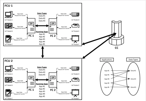
Let us consider the following example to expand the equation in element-wise to see the linearity of the problem. There exists 5 applications using 3 data types running in 2 FCUs, and there is an CC between these 2 FCUs. This example is given graphically in Figure 4.2.
CC IoT Node D IoT Node E IoT Node F FC 2 Apps Data Request & Transfer
Apps Data Request & Transfer
Apps Data Request & Transfer
DP FC 1 IoT Node A IoT Node B IoT Node C Apps Data Request & Transfer
Apps Data Request & Transfer
Apps Data Request & Transfer
DP IoT Node D IoT Node E IoT Node F FC 2 Apps Data Request & Transfer
Apps Data Request & Transfer
Apps Data Request & Transfer
DP FC 1 IoT Node A IoT Node B IoT Node C Apps Data Request & Transfer
Apps Data Request & Transfer
Apps Data Request & Transfer
DP IoT Node D IoT Node E IoT Node F FC 2 Apps Data Request & Transfer
Apps Data Request & Transfer
Apps Data Request & Transfer
DP FC 1 IoT Node A IoT Node B IoT Node C Apps Data Request & Transfer
Apps Data Request & Transfer
Apps Data Request & Transfer
DP Running Apps App #1 App #2 App #3 App #4 App #5 Data Types Data #1 Data #2
Data #3 IoT Node D
IoT Node E IoT Node F
FC 2
Apps Data Request & Transfer
Apps Data Request & Transfer
Apps Data Request & Transfer
DP FC 1 IoT Node A IoT Node B IoT Node C Apps Data Request & Transfer
Apps Data Request & Transfer
Apps Data Request & Transfer
DP Running Apps App #1 App #2 App #3 App #4 App #5 Data Types Data #1 Data #2 Data #3 Data Types Data #1 Data #2 Data #3 Running Apps App #1 App #2 App #3 App #4 App #5 App #1 App #2 App #3 App #4 App #5 Data #1 Data #2 Data #3
Applications Data Types
Figure 4.2: An example of network & data dependency graph (2 FCUs, 1 CC, 5 applications and 3 data types).
If we put the numbers in Equation 4.26, we get the following: 1 C 5 X i=1 1 bi 2 X k=1 3 X y=1
ark,isafi,y( 3
X
z=1
lz,(1+k)py,z) (4.27)
After writing all the elements together with constant C and column sum vector B in the equation, we obtain the following:
1 C 5 X i=1 1 bi 2 X k=1 3 X y=1
ark,isafi,y( 3 X z=1 lz,(1+k)py,z) = 1 C 5 X i=1 1 bi 2 X k=1 3 X y=1
ark,isafi,y(l1,(1+k)py,1+ l2,(1+k)py,2+ l3,(1+k)py,3)
= 1 C 5 X i=1 1 bi 2 X k=1
ark,i(safi,1l1,(1+k)p1,1+ safi,1l2,(1+k)p1,2+ safi,1l3,(1+k)p1,3+
safi,2l1,(1+k)p2,1+ safi,2l2,(1+k)p2,2+ safi,2l3,(1+k)p2,3+
safi,3l1,(1+k)p3,1+ safi,3l2,(1+k)p3,2+ safi,3l3,(1+k)p3,3)
= 1 C 5 X i=1 1 bi
(ar1,isafi,1l1,2p1,1+ ar1,isafi,1l2,2p1,2+ ar1,isafi,1l3,2p1,3+
ar1,isafi,2l1,2p2,1+ ar1,isafi,2l2,2p2,2+ ar1,isafi,2l3,2p2,3+
ar1,isafi,3l1,2p3,1+ ar1,isafi,3l2,2p3,2+ ar1,isafi,3l3,2p3,3
ar2,isafi,1l1,3p1,1+ ar2,isafi,1l2,3p1,2+ ar2,isafi,1l3,3p1,3+
ar2,isafi,2l1,3p2,1+ ar2,isafi,2l2,3p2,2+ ar2,isafi,2l3,3p2,3+
ar2,isafi,3l1,3p3,1+ ar2,isafi,3l2,3p3,2+ ar2,isafi,3l3,3p3,3)
. . .
Equation continues, and it is obvious that there exists no multiplication be-tween any of the decision variables which concludes that the proposed formulation is linear.
4.4
Summary
We start this chapter with a mathematical model of the data placement problem explained in Chapter 3. We can obtain optimal solutions by using this model with any of the linear-solvers available. As it can be clear in the performance evaluation part that finding optimal solution become time-consuming when the values of the parameters increase, so we propose four heuristic algorithms as an alternative to this optimization model in Chapter 5.
Since we envision that the gap between the number of different applications and data types increases, we define a metric called excess use to be used for defining the dependencies of applications and data types.
At the end of this chapter, we expand the complex mathematical equation with a numerical example to prove its linearity. This guarantees when the math-ematical model is solved with linear solvers, the output is optimal, and the best decisions given in the performance evaluation part are comprised of these results. In other words, we evaluate our proposed algorithms according to the linear model given in this chapter.