6 IEEE TRANSACTIONS ON CIRCUITS AND SYSTEMS-I: FUNDAMENTAL THEORY AND APPLICATIONS, VOL. 42, NO. I , JANUARY 1995
Pole-Zero Computation
in Microwave Circuits
Using Multipoint Pad6 Approximation
Mustafa Celik, Ogan Ocali, Mehmet A. Tan, Senior Member, IEEE, and Abdullah Atalar, Senior Member, IEEE
Abstruct- A new method is proposed for dominant pole- zero (or pole-residue) analysis of large linear microwave circuits containing both lumped and distributed elements. The method is based on a multipoint Pad6 approximation. It finds a reduced- order rational s-domain transfer function using a data set ob- tained by solving the circuit at only a few frequency points. We propose two techniques in order to obtain the coefficients of the transfer function from the data set. The proposed method provides a more efficient computation of both transient and frequency domain responses than conventional simulators and more accurate results than the techniques based on single-point PadC approximation such as asymptotic waveform evaluation.
I. INTRODUCTION
OLE-ZERO computation in a linear circuit is alge-
P
braically equivalent to the computation of the eigenvalues of a circuit matrix. There exist many numerical eigenvalue algorithms including QR, QZ, deflation-QZ, Muller, MD-QR algorithms. A detailed comparison of them is given in [l].Another approach in pole-zero computation is to obtain a
rational network function in the s-domain and find the poles and zeros from the polynomials of this rational function by means of a standard root finding algorithm. A review of symbolic frequency domain network analysis methods can be found in [6]. Among these methods the most popular one is
the numerical interpolation method. It is based on polynomial interpolation with arbitrary selection of frequency points. It is shown in [7] that the best result is obtained when the interpolation points are uniformly distributed on the unit circle, which is known as interpolation using FFT algorithm. Most of the symbolic analysis methods, including the interpolation algorithm, try to compute an exact form of the network functions in the frequency domain.
The methods mentioned above are not practical for mi- crowave circuits for two reasons:
1) Usually, practical microwave circuits are of large size, therefore difficult to analyze. Even a simple circuit may have a very large equivalent circuit due to highly complex device models and parasitic elements that may be obtained by means of layout extractors.
2 ) Circuits which contain distributed elements are infinite-
dimensional systems and have an infinite number of poles. Therefore, the methods which attempt to find an exact solution would not be successful.
Manuscript received June 7, 1993; revised March 1, 1994 and September 15, 1994. This work was supported by NATO-SFS project TU-MIMIC. This paper was recommended by Associate Editor Amedeo Premoli.
The authors are with the Department of Electrical and Electronics Engi- neering, Bilkent University, Bilkent 06533, Ankara, Turkey.
1057-7 122/95$04
One solution to these problems is the dominant pole-zero (or pole-residue) approximation using the Asymptotic Waveform Evaluation (AWE) [ 2 ] method. The AWE technique employs
a form of PadC approximation to approximate the behavior of the higher order linear circuit with a reduced order model. The moments of the circuit, which result from a Taylor series expansion of the circuit response about s = 0, are matched to a reduced order rational function. Since the moments convey information about the low-frequency characteristics of the circuit, the AWE technique can only extract the low- frequency poles. However, for some applications, e.g., the interconnect circuits, the mid and high frequency ranges are more important.
In order to improve the accuracy and generality of the AWE method, many techniques have been proposed. It has been extended to handle lossy coupled transmission lines 131,
1141, [lo]. In addition to the moments, the Markov parameters, which are the coefficients of the Taylor series expansion at s =
m, are used to improve the accuracy of the transient response near
t
= 0 [5]. Moment matching techniques have been refined in order to obtain accurate and stable low-frequency poles [11]-[13].Recently, Chiprout and Nakhla have introduced the complex frequency hopping (CFH) technique [9] in order to find all of the dominant poles within the frequency range of interest. In this technique, a number of single point expansions is performed at different frequency points. The expansion points are chosen on the j w axis using a binary search technique and then the poles which are considered to be accurate under some criteria are collected.
This paper proposes a new pole-zero (or pole-residue) ap- proximation technique for the analysis of large linear circuits. The novelty of this method over AWE based methods is that the approximation holds for the entire frequency range under consideration rather than for the low frequencies only. This method also provides a better approximation than the previously proposed work which uses multipoint moment matching methods such as the CFH technique, as will be shown to reader in the following sections.
The proposed approach requires the solution of the circuit matrix at a few frequency points. The derivatives of the network function with respect to s are obtained efficiently from these solutions. By using these derivatives at different complex frequency points, a multipoint Pad6 approximation is used in order to obtain a reduced order s-domain network function. Poles and zeros (or poles and residues) can be found from this rational network function using standard techniques.
CELIK er al.: POLE-ZERO COMPUTATION IN MICROWAVE CIRCUITS 7
In the next section, the order reduction technique is ex- plained briefly. Frequency-shifted moments are defined in Section 111. We propose two methods for the calculation of the coefficients of the network function in Section IV. Practical and numerical considerations of the proposed method are given in Section V. In Section VI we present some examples to show the performance of the proposed method.
11. ORDER REDUCTION
Consider a linear system modeled by a coupled set of linear algebraic equations in Laplace domain,
T(s)x = w (1)
where T is the system matrix, the vector x is the system
response and the vector w is the system excitation. In gen- eral, the system matrix T is an arbitrary function of s. Let
the system output be any linear combination of the system response,
H = dTx. (2)
Using Cramer's rule one can obtain
(3) If the elements of the system matrix are polynomials in s (e.g., in lumped networks T = T1
+
ST^), the expansion of the determinants in (3) leads to polynomials in s ,(4) In this paper, we consider the circuits containing distributed components as well as lumped elements. Those circuits can be regarded as infinite-dimensional systems and the network functions for an infinite-dimensional system cannot be ex- pressed as a ratio of two polynomials of finite-degree. Our aim is to approximate the network function H ( s ) - regard- less of whether it is a rational or irrational function of s, with a rational function
B(s)
which has approximately the same frequency characteristics as the original circuit. Let the approximate function be of the formbo
+
b l s+
. . .
+
bq-1sq-'H ( s ) = ( 5 )
1
+
a1s+
. . .
+
a&Since there are 29 parameters to compute in the reduced model, we need 2q constraints from the actual circuit. In the AWE technique 2q unknowns are calculated by matching the first T moments and the first (2q - T ) Markov parameters of the
original circuit to the approximate rational function [ 5 ] .
In this work, we propose a method which uses a data set obtained from the circui! to construct the approximate s-domain rational function, H ( s ) . This data set contains the
frequency-shifed moments obtained at different complex fre-
quency points. In the following section, we present the eval- uation of the frequency-shifted moments.
111. FREQUENCY-SHIFTED MOMENTS
The system response x(s), can be expanded into a Taylor
series at s = S k as:
m
i=O
provided that x(s) is analytic at s = Sk. The coefficient xki in (6) is called the vector of ith frequency-shifted moments' at s = S k and
(7) The first moment vector is the solution of the circuit at s = s k , X ~ O = T - ' ( s ~ ) w . (8)
It can be shown that the higher order moments can be evaluated recursively as,
. .
r = l
where superscript ( T - ) indicates the rth derivative with respect to s. If the circuit contains only lumped components, then
T(') = 0 for T-
>
1. If it contains distributed elements, then the derivatives can be found efficiently using either the eigenvalue moment method [3],[ 141 or the matrix exponential method [lo].are obtained from the moment vectors xki's as,
The moments for a particular output of the circuit at s = S k .
where nk is the number of the moments at s = sk. We denote the point s = 0 by S O and the moments at s = 0 are represented with moi. Note that, the frequepcy-shifted moments at s = sz
are complex conjugates of the frequency-shifted moments at
s = sk. We represent the frequency point
SE
by s - k and the moments at s = s-k by m - k i . Let N be the total number of moments, then we haven n
k=-n k = l
where n is the number of expansion points in the upper half
s-plane.
IV. MULTIPOINT MOMENT MATCHING
We match the moment set, which contains N frequency-
shifted moments obtained from 2n
+
1 points, to a qth order proper rational function (q = N / 2 , which implies N shouldbe even), which is denoted by [(q - l)/q]:
k = - n
,..,
0,..,
n We propose two methods for the calculation of the coefficients of the rational function. In the first method a set of linear8 IEEE TRANSACTIONS ON CIRCUITS AND SYSTEMS-1: FUNDAMENTAL THEORY AND APPLICATIONS, VOL. 42, NO. 1 , JANUARY 1995
equations is obtained for the coefficients and solved directly. The second method finds the coefficients in a recursive manner without requiring a matrix inversion.
matrix equation is formed:
A. Method 1
In this part we will show that finding the coefficients of the rational function is equivalent to solving a set of linear equations.
Let us first consider the one-point moment matching case at s = sk. If we write the polynomials of the rational function in terms of i = s - S k rather than s, we obtain:
60
+
b 1 i+
...
+
b q - $ - l - - &I+
i i 1 i+
...
+
i i q i q m k O+
m k l i+
...+
m k ( n k - l ) i n k - l+
0 ( i 7 ' n ) , (12) where, 6 0 = 1+
E;-
a&6
t --E"-'
l=z bl(;)s;-z, (13) iiz =E;='=,
a l ( Z ) S ; - Z ,-11
i = 1 , 2 , . . . q i = 0 , 1 ,...
9 - 1 .Multiplying the denominator polynomial with right hand side in (12) and equating the coefficients gives
bo = mkoao
-
b n b - 1 - m k 0 6 ~ ~ ~ - 1
+
...+
m k ( n ~ - l ) ~ o or in the matrix form,Mkc = m k . (15)
In (151, c = [bo...b,-lal . . . a , ] T is the coefficient vector
and,
m k = [ m k o
. . .
m k ( r ~ ~ - l ) ] *and the n k by N matrix Mk is equivalent to
[C1
i
C Z BC2 B C a ] . where ...I
mkO B = [mkl mkO : mk(nk-1) mk(nk-2) mkOand C1, Cz and C3 are defined as: [ C I
I
cz
I
C a ] =Note that, M-k = M; and m-k = m;, Finally, collecting the equations obtained from all points, the following N by N
The solution of this matrix equation yields the coefficients of the rational transfer function we are seeking.
B. Method 2
Alternatively, the coefficients of the rational function can be found by means of a recursive computation scheme starting from a polynomial which interpolates the given data set. This method corresponds to the computation of a cross- diagonal sequence in Pad6 table, i.e., it gives all [m/Z] Pad6 approximations such that m
+
1 = N-
1.We denote the rational function that corresponds to the [(N-l-Z)/Z] Pad6 approximation by p l / q l . In other words, for a denominator polynomial the degree is its subscript and for a numerator polynomial the degree is the difference between its subscript and N - 1. Now, let us suppose that the rational function p l / q l interpolates the given data set. That is,
lc
= -n,..,
0, ..n Let us also define the polynomial g( s ) of degree N as71
k=-n
Now, assuming p l ( s ) and q ( s ) are co-prime with g ( s ) , we claim that if
P l ( s ) q m ( s )
-
P m ( S k l ( S ) = d s ) r ( s ) , (22)where ~ ( s ) is a polynomial such that deg[r(s)] = max(l -
m - 1, m - 1 - l), then the rational function p , / q , also interpolates the given set. We can prove this claim as follows. Dividing both sides of (22) by q l ( s ) q m ( s ) we obtain,
(23)
Pl(s)
- P , o = g(s)r(s)q l ( s ) 4 m ( s ) 4 1 ( . 5 ) 4 m ( S ) . From the definition of g ( s ) we have
IC
= -n, ..,0, ..n. (24) Therefore,i = 0,1,
..,
nk - 1, IC = -72, ..,0, ..TI,. (25) The converse of the claim is also true. That is, if p l / q l andp , /qm are two rational polynomials interpolating the moment
CELIK et al.: POLE-ZERO COMPUTATION IN MICROWAVE CIRCUITS 9 Now, we can construct our method as follows. Let pl/ql and
p l P l / q l - be two consecutive solutions, then (22) becomes: P l ( s ) q l - l ( s ) - P l - l ( s ) q l ( s ) = s ( s ) r o , (26) where T O is any real number. Now if we divide the polynomial p l - l ( s ) by p l ( s ) we obtain
P l - l ( S ) = P l ( S ) C ( S ) - 4 s ) , (27) where, c ( s ) is the quotient polynomial with degree 1 and d ( s )
is the remainder polynomial with degree N - 1 - 2. If we add and subtract the polynomial p l ( s)ql ( s ) c ( s ) to the left hand
side of (26) we obtain
(28) where e ( s ) = q l ( s ) c ( s ) - q l - I ( s ) with degree 1+1. Now since
d ( s ) and e(s) have degrees of N - 1 - 2 and 1
+
1, respectively and since they satisfy (22), we conclude that d / e is nothingbut [ ( N - 1 - 2)/(1
+
l ) ] Pad6 approximation:d ( s ) q l ( s ) - P l ( s ) e ( s ) = s ( s ) r o ,
P l + l ( S ) = 4 s ) (29) q l + l ( s ) = 4 s ) . (30) As a summary, given p l - l / q l - I and p l / q l , we can find pl+l/ql+1 simply by evaluating one polynomial division, one polynomial multiplication and one polynomial addition. The first two approximations are found as follows: Let f ( s ) be a polynomial of degree N - 1 interpolating the computed moment set,
IC = -n
,..,
O,..n. (31) The polynomial f ( s ) is, in fact, [ ( N - 1)/0] Pad6 approxi- mation and to obtain [ ( N - 2)/1] approximation we rewrite (26),P l ( S ) - f(s)q1(s) = g(s)ro, (32) which means that the quotient of the division of g(s) by f ( s ) gives q1(s) and the remainder is p l ( s ) . Therefore, having found the data interpolating polynomial
f
( s ) , we can compute recursively the cross diagonal sequence of the Pad6 table.V. PRACTICAL CONSIDERATIONS
In the previous sections, we treated the subject theoret- ically. Now, we will discuss some topics on the practical implementation of the proposed method.
A. Calculation of Frequency-Shijled Moments
A recursive scheme for computing the frequency-shifted moments at a point is given in (9). Since the LU factorization of the circuit matrix T(sk) is known from the solution of the first moment vector, each higher order moment vector can be obtained by one forward and one back substitution (FBS) only. Totally, we need n
+
1 LU decompositions of the circuit matrix which is equivalent to obtaining the ac response of the circuit at dc and n points. In addition to LU decompositions we alsoneed ni FBS’s in order to calculate the N moments.
B. Selection of Frequency Points
A crucial step in our method is the selection of frequency points. Only the poles close to the j w axis are important in both time and frequency analyses. Therefore, we choose the expansion points on the j w axis. Once the frequency region of interest is specified, which is generally between dc and a maximum frequency, the location and the number of expansion points can be chosen using the complex frequency hopping (CFH) algorithm [9]. This algorithm first performs one-point expansions at the points s = 0 and s = j w m a z . The poles are
calculated separately from these expansions and if there exists any common pole, then the search is completed. Otherwise, more frequencies are selected using a binary search and, an expansion is performed at every new point until every two suc- cessive expansions result in at least one common pole. In the CFH method, the poles about an expansion point are calculated independently from the other expansions, and this conse- quently decreases the accuracy. In contrast, in our algorithm, all of the poles and the corresponding residues are obtained considering all the expansion points simultaneously. This approach yields a more compact and accurate approximation. The CFH technique gives the number of accurate poles about an expansion point. We can choose the number of moments at each frequency point using this information but not less than 8 moments at one point. Having chosen the expansion points and the number of moments at each point, we can find the coefficients of the rational transfer function using one of the two methods presented in Section IV.
C. Finding the Coeflcients Using Method 1
The complex conjugate of every row also exists in (19). Therefore, this N by N complex equation set is equivalent to
an N by N real equation set and can be solved using ordinary
elimination algorithms.
Since our method is proposed for relatively complex cir- cuits, the orders of approximations (10 N 50) are generally
large compared to the orders of typical approximations (< 12) seen in the AWE technique. Hence, very large numbers can appear in the entries of the matrix given in (19) because of the powers of the expansion points, and consequently, the matrix can become ill-conditioned. Therefore, we use double precision arithmetic, and, we also perform a frequency scaling such that the absolute values of the expansion points,
I
S k l’s, are reduced to around unity.Another important topic is the stability of the approxi- mated poles. Similar to the AWE technique, multipoint Pad6 approximations may also result in spurious right hand side poles. When some unstable poles appear in an approximation, we discard them and solve a new matrix equation for the coefficients of the numerator polynomial. The new matrix equation is obtained as follows. First, let q’ be the number of stable poles of the q approximated poles. Now, let us rewrite (19) in the form,
(33) or
10 IEEE TRANSACTIONS ON CIRCUITS AND SYSTEMS-I: FUNDAMENTAL THEORY AND APPLICATIONS, VOL. 42, NO. I , JANUARY 1995
where the vector b’ contains the coefficients of the numerator polynomial to be solved, the vector a’ corresponds to the coefficients of the stable denominator polynomial and the other primed quantities are obtained in a similar manner defined in Section IV, but this time the number of moments are reduced such that 2q’ = 7th
+
2E;=,
nk. Equation (34) isoverdetermined and a solution in the least square sense can be obtained. However, this solution does not exactly match the first q’ moments. Therefore, we form the primed quantities in
(34) by taking the first n k / 2 moments from each point which
results in a q’ by q’ matrix equation.
D. Finding the CoefJicients Using Method 2
In contrast to the first one, this method does not require any matrix inversion. It is more efficient than the first method. Moreover, this method allows a search on the Pad6 table in order to choose stable and accurate approximations. The major difficulty with this method is the construction of the data interpolation polynomial,
f(
s). This polynomial is obtained using the method of divided differences [8] and, generally, itis numerically hard to obtain the coefficients for higher order interpolations. Our experiments show that approximations having orders up to about 20-25 can be found. However, the first method yields accurate results up to 40-50 poles. E. Finding the Poles and the Residues
After having obtained the coefficients of the network func- tion, to find the poles and residues, a partial fraction de- composition routine is employed which requires a polynomial factorization with an associated extra CPU time. This extra cost becomes important only when the order of approximation must be increased to about 50. For this size, this task is about
1.6 million floating point operations. Even in this case, this is
less than the CPU time required for the moment computation. As the circuit size grows, moment computation gets more costly, but the cost of the polynomial factorization remains the same.
The obtained set of poles and residues may be inaccu- rate due to round-off errors both in the computation of the coefficients of the network function and in the polynomial factorization. This set of poles and residues can be verified for accuracy by using an error criterion defined in the following. Consider the approximated transfer function:
where the p j are the q approximate poles, and the k j their corresponding residues. Then, the approximate moments of this transfer function can be computed as,
IC
= -n,..,
O,..n. (36)In the absence of round-off errors, we should have
i = O , l , . . , n k - l , r i Z k i = mki, IC = -n, ..,O, ..n (37) 0, 1 exact Methcd 1 AWE _ _ _
- - I
C -60 -70 -80Fig. 1. Frequency response of the lowpass filter.
where mki are the exact moments obtained from the circuit. A normalized error can be defined as
The error increases as the order of approximation increases and an error beyond a tolerance limit indicates that the approxima- tion is inaccurate. In this case, a new lower order multipoint Pad6 approximation should be performed. However, our ex- periments have revealed that, even for an approximation of order 50, this error is less than 1 x which corresponds to a good accuracy.
VI. EXAMPLES
The following examples demonstrate the performance of the proposed method on both transient and frequency analyses.
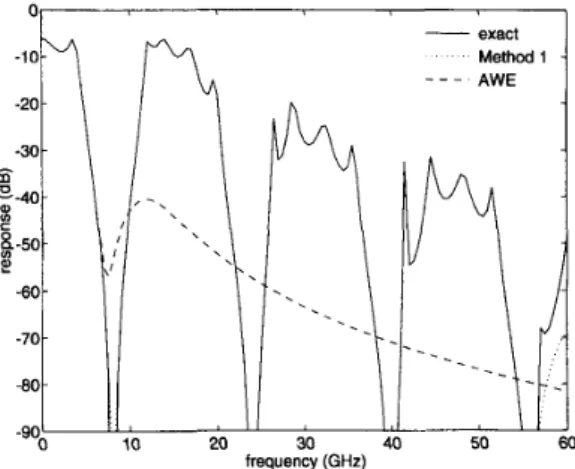
Example I : The first example is a lowpass filter imple-
mented with transmission lines. It has a cutoff frequency of
4 GHz. Because of the repetitive properties of the transmission lines, the response is significant also at higher frequencies.
The actual frequency response of the filter is shown in Fig. 1 . Applying the enhanced moment matching techniques [ll], we found that the best AWE result is the [6/9] Pad6
approximation which is plotted in Fig. 1 . We have chosen the
maximum frequency as 50 GHz, and, found the expansion points to be 0, 12.5, 25, 37.5, and 50 GHz using CFH
technique (so = 0, s1 = j27r12.5
x
l o 9 , s-1 = -j27r12.5x
lo9,
...,
s4 = j27r5Ox1O9, s V 4 = -j27r5Ox1O9). Solving (19),we have found the 47th order approximation (no = 14,ni = 10, for i = 1, - 1 ,
...,
4 , -4) which resulted in 41 stablepoles. Then solving (34), we have obtained the stable [40/41]
approximation whose frequency response is also shown in Fig. 1 .
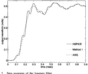
The step response of the filter is also computed from the approximations mentioned above. The results are shown in Fig. 2 together with the HSPICE simulation result for
comparison.
Using this circuit again, we have compared the accuracies of the CFH technique and our first method. Let 0 and 1 1 GHz be
CELIK er al.: POLE-ZERO COMPUTATION IN MICROWAVE CIRCUITS 0.5 0.4 - Y
-
P2
€0.3- s 11 - - Proposed method HSPICE CFH method Method 1j
0.1t
,I
A W E _ _ _ 0 0.1 0.2 0.3 0.4 0.5 0.6 0.7 0.8 0.9 time (nsec) A W E _ _ _ 0 0.1 0.2 0.3 0.4 0.5 0.6 0.7 0.8 0.9 time (nsec)Fig. 2. Step response of the lowpass filter.
I -2.3329803591e11 I I I -1.4459214949ell I
1
-9.2186239031e08 f j1.231099147Oell -4.2213073890e09 f j1.0631300764ell -5.131872946449 f j8 7044023156e10 -4.2316598128e09 f j1.0636483876e11 -5.131869963749*
j8 7044023398elOc
-1.9776350608eO9 f j7.5409512193elO -1.9776350608eO9 f j7.5409512192elOI -2.2627219713elO
*
j3.7198003498e10 I -2.2790993205elO f j3.7221048203elO I I -3.6133889942elO I -3.6137020835e10 I I -2.7169584289p09 zi i2.3731095682elO 1 -2.716954635Oe09 f i2.3731023229elO 1I -9.7407610673e09 1 -9.7407610672e09 I
two hopping frequencies. Then, following the steps explained in [9], we have found 12 accurate poles using 16 real moments (s = 0) and 16 complex moments (s = j27r11 x lo9). Our method, using 16 real moments and 12 complex moments, has been able to find a stable 18-pole approximation. The approx- imated poles are listed in Table I for reference. The accuracy of these two sets of poles and residues have been compared using the error criterion given in (38). The errors have been calculated as cm = 1.554 x 10⁻¹ and ,t = 7.035 x 10-l2, in CFH's and our results, respectively. Normalized errors in the frequency response2 with respect to actual response are plotted in Fig. 3. Since the filter has a zero at 8 GHz, normalized errors become very large around that frequency. As it is seen from the figure, the accuracy is considerably improved by using multipoint moment matching rather than collecting the poles from a set of single-point moment matches. The price we pay is to solve an extra 40 by 40 matrix. In comparison to the other computations this is a very small price.
Example 2: We consider the interconnect circuit shown in
Fig. 2 of [3]. It contains 7 transmission lines, 8 inductors, 12 capacitors and 9 resistors.
@( J ) ) / H ( J U!)
I.
*Normalized error in frequency response is defined as, E, = ~ ( H ( J Z P ) -
Fig. 3. Normalized error in the frequency response of the lowpass filter.
-10, - exact Method 1 Method 2 A W E _ _ . _ _ _ 1 2 3 4 5 6 frequency (GHz)
Fig. 4. Frequency response of the interconnect circuit.
Using the CFH technique, we have found the expansion points as 0, 1.25, 2.5, and 5 GHz. Taking 10 moments at each point we have obtained a 35th order approximation or the stable [30/3 11 approximation using the first method proposed in this work. The exact and approximated frequency responses are shown in Fig. 4. The 11th order AWE result is plotted in the same figure.
We have also tested our second method in this circuit. We
have chosen the expansion points as 0, 1.25, and 2.5 GHz, and, found the [17/18] approximation. The result is shown in Fig. 4. In Fig. 5, normalized errors of all approximations are plotted as a function of frequency.
In Fig. 6, we present the step responses obtained from the above approximations. Our results and the HSPICE result are indistinguishable to the resolution of figure. In Fig. 7 the errors of the approximated step responses with respect to the HSPICE result are plotted. Figs. 5 and 7 show clearly how far the accuracy is improved by solving the matrix equation directly.
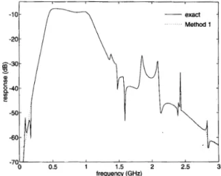
Example 3: A circuit which contains six band-pass filters in parallel is considered. It has a total of 20 transmission lines, 23 inductors, 32 capacitors and 26 resistors. The filters are switched by finite isolation PIN diodes resulting in a very complicated frequency response.
12 IEEE TRANSACTIONS ON CIRCUITS AND SYSTEMS-] FUNDAMENTAL THEORY AND APPLICATIONS, VOL. 42, NO. 1, JANUARY 1995
Fig. 5.
circuit
Normalized errors in the frequency response of the interconnect
- HSPICE Method 1 Method 2 AWE _ _ _ - - - _ 1.5
Fig. 6. Step response of the interconnect circuit
Using CFH technique the expansion points have been found as 0.5, 1 .O, 1.5, 2.0, and 2.5 GHz. Since the circuit has a band- pass type characteristics, the expansion about s = 0 does not give any useful information. Therefore, we have chosen the first expansion point as 0.5 GHz (no = 0). Taking 8 moments at each point we have found a 40th order approximation which resulted 36 stable poles. The magnitude and the phase of the
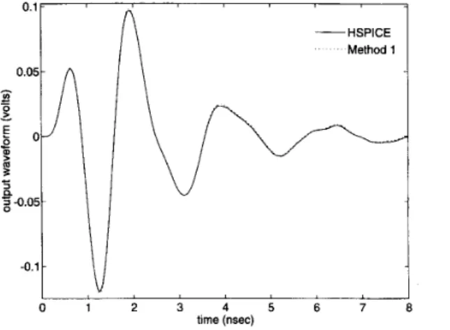
frequency response are compared with the exact response in Figs. 8 and 9. The step response of the filter is shown in Fig. 10 together with the HSPICE result for comparison.
VII. CONCLUSIONS
A new dominant pole-zero (or pole-residue) computation method for microwave circuits has been presented. This method uses a multipoint Pad6 approximation to find a reduced order s-domain network function. In order to find the coefficients of the multipoint Pad6 approximant, we proposed two techniques. The poles obtained from the network function are not necessarily low-frequency approximations as it is the
I
0.5 1 1.5 2
time (nsec)
Fig. 7. Errors in the step responses of the interconnect circuit.
-20t
I
-50 - -60-\
-
exact Method 1I/-
-70;'
0.5 1 1.5 2 2.5 frequency (GHz)Fig. 8. Frequency (magnitude) response of the band-pass filter
2001 I 1 I 0.5 1.5 2 2.5 3 frequency (GHz) Fig. 9.
case in AWE. This method can also be used to compute pole- zero sensitivity in a similar way to the approach presented in [4].
CELIK et al.: POLE-ZERO COMPUTATION IN MICROWAVE CIRCUITS 13
~ HSPICE
Method 1
7 8
Fig. 10. Step response of the band-pass filter
VIII. ACKNOWLEDGMENT
The authors thank the reviewers for their helpful sugges- tions. They especially thank the reviewer who suggested the use of the complex frequency hopping algorithm in the method presented here.
REFERENCES
S. B. Haley, “The generalized eigenproblem: Pole-zero computation,” Proc. IEEE, vol. 76, pp. 103-120, Feb. 1988.
L. T. Pillage and R. A. Rohrer, “Asymptotic waveform evaluation for timing analysis,’’ IEEE Trans. Computer-Aided Design, vol. 9, no. 4, pp. 352-366, Apr. 1990.
T. K. Tang and M. S. Nakhla, “Analysis of high-speed VLSI inter- connects using the asymptotic waveform evaluation technique,” IEEE Trans. Computer-AidedDesign, vol. 11, no. 3, pp. 341-352, Mar. 1992. J. Y. Lee, X. Huang, and Ronald A. Rohrer, “Pole and zero sensitivity calculation in asymptotic waveform evaluation,” IEEE Trans. Computer- Aided Design, vol. 11, no. 5, pp. 586597, May 1992.
X. Huang, V. Raghavan, and R. A. Rohrer, “AWEsim: A program for the efficient analysis of linear(ized) circuits,” in Tech. Dig. ICCAD’90, Nov. 1990, pp. 534-537.
T. Matsumoto, “Symbolic network analysis,” in Analog Methods for Computer-Aided Circuit Analysis and Diagnosis. Marcel Dekker, 1988.
J. Vlach and K. Singhal, &omputer Methods for Circuit Analysis and Design. New York: Van Nostrand Reinhold, 1983.
S. D. Conte and C. de Boor, Elementary Numerical Analysis. Singa- pore: McGraw-Hill, 1981.
E. Chiprout and M. Nakhla, “Transient waveform estimation of high- speed MCM networks using complex frequency hopping,” inProc. Multi-Chip Module Con$, Mar. 1993.
__, “Addressing high-speed interconnect issues in asymptotic wave- form evaluation,” in Proc. Design Automat. Con$, May 1993.
- , “Generalized moment-matching methods for transient analysis of interconnect networks,” in Proc. Design Automat. Con$, June 1992. -, “Optimal pole selection in asymptotic waveform evaluation,” in Proc. Int. Symp. Circuits, Syst. 1992 (ISCAS ’92), May 1992.
D. F. Anastasakis, N. Gopal, S. Y. Kim, and L. T. Pillage, “On the stability of approximations in asymptotic waveform evaluation,” in Proc. Design Automat. Con$, June 1992.
J. E. Bracken, V. Raghavan, and R. A. Rohrer, “Simulation distributed elements with asymptotic waveform evaluation,” in Proc. IEEE Int. Microwave Symp. (MTT-S), June 1992.
Mustafa Celik was born in Konya, Turkey, in 1966.
He received the B.S. degree from the Middle East Technical University, Ankara, Turkey, in 1988, and the M.S. and Ph.D. degrees from Bilkent University, Ankara, Turkey, in 1991 and 1994, respectively, all in electrical engineering.
His research interest is in circuit simulation.
Ogan Ocali was born in Izmir, Turkey, in 1965.
He received the B.S. degree from the Middle East Technical University, Ankara, Turkey, in 1987, and the M.S. in electrical engineering from Bilkent University in 1990. He is currently working toward the Ph.D. degree in electrical engineering at Bilkent University.
His research interests include sampled-data con-
trol theory and computer-aided simulation of elec- tronic circuits.
Mehmet A. Tan (S’85-M’88-SM’94) was born in
1959 in Adana, Turkey. He received the B.S. and M.S. degrees from Istanbul Technical University, Is- tanbul, Turkey, in 1980 and 1982, respectively, and the Ph.D. degree from the University of Minnesota, Minneapolis, MN, in 1988.
In 1988, he joined the faculty of the Department of Electrical and Electronics Engineering at Bilkent University, Ankara, Turkey, where he is currently Associate Professor of Electrical Engineering. His active research interests include analog integrated -
-circuits and signal processing, electronic implementation of artificial neural networks, and computer-aided design of electronic circuits. .
Dr. Tan served as Chairman of IEEE Circuits and Systems Turkey Chapter from 1992 to 1994. He is currently the Chairman of IEEE Turkey Section.
Abdullah Atalar (M’88-SM’90) was born in
Gaziantep, Turkey, in 1954. He received the B.S. degree from the Middle East Technical University, Ankara, Turkey, in 1974, and the M.S. and Ph.D. degrees from Stanford University, Stanford, CA, in 1976 and 1978, respectively, all !n electrical engineering. His thesis work was on reflection acoustic microscopy.
From 1978 to 1980, he was first a Post-Doctoral Fellow and later an Engineering Research Associate at Stanford University, continuing his work on acoustic microscopy. For 8 months he was with Hewlett Packard Labs., Palo Alto, CA, engaged in photoacoustics research. From 1980 to 1986, he was on the faculty of the Middle East Technical University as an Assistant Professor. From 1982 to 1983, on leave from the University, he was with Ernst Leitz Wetzlar, Wetzlar, West Germany, where he was involved in the development of the commercial acoustic microscope. In 1986 he joined the Bilkent University and served in the founding of the Electrical and Electronics Engineering Department where he is currently a Professor. His current research interests include acoustic imaging, linear acoustics, and computer-aided design in electrical engineering.