Pipelined fission for stream programs with dynamic selectivity and partitioned state

(1)

Contents lists available atScienceDirect

J. Parallel Distrib. Comput.

journal homepage:www.elsevier.com/locate/jpdc

Pipelined fission for stream programs with dynamic selectivity and

partitioned state

B. Gedik

∗

,

H.G. Özsema,

Ö. Öztürk

Department of Computer Engineering, Bilkent University, 06800, Ankara, Turkey

h i g h l i g h t s

• Formalizes the pipelined fission problem for streaming applications. • Models the throughput of pipelined fission configurations.

• Develops a three-stage heuristic algorithm to quickly locate a close to optimal pipelined fission configuration. • Experimentally evaluates the solution and demonstrate its efficacy.

a r t i c l e i n f o Article history:

Received 19 February 2015 Received in revised form 2 December 2015 Accepted 3 May 2016 Available online 14 May 2016

Keywords:

Data stream processing Auto-parallelization Pipelining Fission

a b s t r a c t

There is an ever increasing rate of digital information available in the form of online data streams. In many application domains, high throughput processing of such data is a critical requirement for keeping up with the soaring input rates. Data stream processing is a computational paradigm that aims at addressing this challenge by processing data streams in an on-the-fly manner, in contrast to the more traditional and less efficient store-and-then process approach. In this paper, we study the problem of automatically parallelizing data stream processing applications in order to improve throughput. The parallelization is automatic in the sense that stream programs are written sequentially by the application developers and are parallelized by the system. We adopt the asynchronous data flow model for our work, which is typical in Data Stream Processing Systems (DSPS), where operators often have dynamic selectivity and are stateful. We solve the problem of pipelined fission, in which the original sequential program is parallelized by taking advantage of both pipeline parallelism and data parallelism at the same time. Our pipelined fission solution supports partitioned stateful data parallelism with dynamic selectivity and is designed for shared-memory multi-core machines. We first develop a cost-based formulation that enables us to express pipelined fission as an optimization problem. The bruteforce solution of this problem takes a long time for moderately sized stream programs. Accordingly, we develop a heuristic algorithm that can quickly, but approximately, solve the pipelined fission problem. We provide an extensive evaluation studying the performance of our pipelined fission solution, including simulations as well as experiments with an industrial-strength DSPS. Our results show good scalability for applications that contain sufficient parallelism, as well as close to optimal performance for the heuristic pipelined fission algorithm.

1. Introduction

We are experiencing a data deluge due to the ever increasing rate of digital data produced by various software and hardware sensors present in our highly instrumented and interconnected world. This data often arrives in the form of continuous streams.

∗_{Corresponding author.}

E-mail addresses:bgedik@bilkent.edu.tr(B. Gedik),

habibe.ozsema@bilkent.edu.tr(H.G. Özsema),ozturk@bilkent.edu.tr(Ö. Öztürk).

Examples abound, such as ticker data [41] in financial markets, call detail records [7] in telecommunications, production line diagnostics [3] in manufacturing, and vital signals [35] in healthcare. Accordingly, there is an increasing need to gather and analyze data streams in near real-time, detect emerging patterns and outliers, and take automated action. Data stream processing systems (DSPSs) [37,20,36,1,5] enable carrying out these tasks in a natural way, by taking data streams through a series of analytic operators. In contrast to the traditional store-and-process model of data management systems, DSPSs rely on the process-and-forward model and are designed to provide high throughput and timely response.

http://dx.doi.org/10.1016/j.jpdc.2016.05.003

(2)

Since performance is one of the fundamental motivations for adopting the stream processing model, optimizing the throughput of stream processing applications is an important goal of many DSPSs. In this paper, we study the problem of pipelined

fission, that is automatically finding the best configuration of

combined pipeline and data parallelism in order to optimize application throughput. Pipeline parallelism naturally occurs in stream processing applications [39]. As one of the stages is processing a data item, the previous stage can concurrently process the next data item in line. Data parallelization, aka.

fission, involves replicating a stage and concurrently processing

different data items using these replicas. Typically, data parallelism opportunities in streaming applications need to be discovered (to ensure safe parallelization) and require runtime mechanisms, such as splitting and ordering, to enforce sequential semantics [33,15].

Our goal in this paper is to determine how to distribute processing resources among the data and pipeline parallel aspects within the stream program, in order to best optimize the throughput. While pipeline parallelism is very easy to take advantage of, the amount of speed-up that can be obtained is limited by the pipeline depth. On the other hand, data parallelism, when applicable, can be used to achieve higher levels of scalability. Yet, data parallelism has limitations as well. First, the mechanisms used to establish sequential semantics (e.g., ordering) have overheads that increase with the number of replicas used. Second, and more importantly, since data parallelism is applied to a subset of operators within the chain topology, the performance is still limited by other operators for which data parallelism cannot be applied (e.g., because they are arbitrarily stateful). The last point further motivates the importance of pipelined fission, that is the need for performing combined pipeline and data parallelism.

The setting we consider in this paper is multi-core shared-memory machines. We focus on streaming applications that pos-sess a chain topology, where multiple stages are organized into a series, each stage consuming data from the stage before and feed-ing data into the stage after. Each stage can be a primitive operator, which is an atomic unit, or a composite [22] operator, which can contain a more complex sub-topology within. In the rest of the pa-per, we will simply use the term operator to refer to a stage. The pipeline and data parallelism we apply are all at the level of these operators.

Our work is applicable to and is designed for DSPSs that have the following properties:

•

Dynamic selectivity: If the number of input data items con-sumed and/or the number of output data items produced by an operator are not fixed and may change depending on the contents of the input data, the operator is said to have dynamic selectivity. Operators with dynamic selectivity are prevalent in data-intensive streaming applications. Examples of such oper-ators include data dependent filters, joins, and aggregations.

•

Backpressure: When a streaming operator is unable to

con-sume the input data items as fast as they are being produced, a bottleneck is formed. In a system with backpressure, this even-tually results in an internal buffer to fill up, and thus an up-stream operator blocks while trying to submit a data item to the full buffer. This is called backpressure, and it recursively prop-agates up to the source operators.

•

Partitioned processing: A stream that multiplexes several sub-streams, where each sub-stream is identified by its unique value for the partitioning key, is called a partitioned stream. An opera-tor that independently processes individual sub-streams within a partitioned stream is called a partitioned operator. Partitioned operators could be stateful, in which case they maintain in-dependent state for each sub-stream. DSPSs that support par-titioned processing can apply fission for parpar-titioned stateful operators—an important class of streaming operators [34,4].

There are several challenges in solving the pipelined fission problem we have outlined. First, we need to formally define what a valid parallelization configuration is with respect to the execution model used by the DSPS. This involves defining the restrictions on the mapping between threads and parallel segments of the application. Second, we need to model the throughput as a function of the pipelined fission configuration, so as to compare different pipelined fission alternatives among each other. Finally, even for a small number of operators, processor cores, and threads, there are combinatorially many valid pipelined fission configurations. It is important to be able to quickly locate a configuration that provides close to optimal throughput. There are two strong motivations for this. The first is to have a fast edit–debug cycle for streaming applications. The second is to have low overhead for dynamic pipelined fission, that is being able to update the parallelization configuration at run-time. Note that, the optimal pipelined fission configuration depends on the operator costs and selectivities, which are often data dependent, motivating dynamic pipelined fission. In this paper, our focus is on solving the pipelined fission problem in a reasonable time, with high accuracy with respect to throughput.

Our solution involves three components. First, we define valid pipelined fission configurations based on application of

fusion and fission on operators. Fusion is a technique used for

minimizing scheduling overheads and executing stream programs in a streamlined manner [25,13]. In particular, series of operators that form a pipeline are fused and executed by a dedicated thread, where buffers are placed between successive pipelines. On the other hand, using fission, series of pipelines that form a parallel

region are replicated to achieve data parallelism.

Second, we model concepts such as operator compatibility (used to define parallel regions), backpressure (key factor in defin-ing throughput), and system overheads like the thread switchdefin-ing and replication costs (factors impacting the effectiveness of paral-lelization), and use these to derive a formula for the throughput.

Last, and most importantly, we develop a heuristic algorithm to quickly locate a pipelined fission configuration that provides close to optimal performance. The algorithm relies on three main ideas: The first is to form regions based on the longest compatible sequence principle, where compatible means that a formed region carries properties that make it amenable to data parallelism as a whole. The second is to divide regions into pipelines using a greedy bottleneck resolving procedure. This procedure performs iterative pipelining, using a variable utilization-based upper bound as the stopping condition. The third is another greedy step, which resolves the remaining bottlenecks by increasing the number of replicas of a region.

We evaluate the effectiveness of our solution based on exten-sive analytic experimentation. We also use IBM’s SPL language and its runtime system to perform an empirical evaluation. Our SPL-based evaluation shows that we can quickly locate a pipelined fis-sion configuration that is within 5%–10% of the optimal using our heuristic algorithm.

In summary, we make the following contributions:

•

We formalize the pipelined fission problem for streaming appli-cations that are organized as a series of stages and can poten-tially exhibit dynamic selectivity, backpressure, and partitioned processing.

•

We model the throughput of pipelined fission configurations and cast the problem of locating the best configuration as a combinatorial optimization one.

•

We develop a three-stage heuristic algorithm to quickly locate a close to optimal pipelined fission configuration and evaluate its effectiveness using analytical and empirical experiments.

(3)

Fig. 1. Pipelined fission terminology.

2. Background

In this section, we summarize the terminology used for the pipelined fission problem, and outline a system execution model that will guide the problem formulation and solution used in the rest of the paper.

2.1. Terminology and definitions

A stream graph is a set of operators connected to each other via streams. As mentioned earlier, we consider graphs with chain

topology in this work.Fig. 1summarizes the terminology used to

define our pipelined fission problem.

There are two operator properties that play an important role in pipelined fission, namely selectivity and state.

•

Selectivity of an operator is the number of items it produces per number of items it consumes. It could be less than one, in which case the operator is selective; it could be equal to one, in which case the operator is one-to-one; or it could be greater than one, in which case the operator is prolific.

•

State specifies whether and what kind of information is main-tained by the operator across firings. An operator could be

state-less, in which case it does not maintain any state across firings. It

could be partitioned stateful, in which case it maintains indepen-dent state for each sub-stream determined by a partitioning key. Finally, an operator could be stateful without a special structure. We name a series of operators fused together as a pipeline. A series of pipelines replicated as a whole is called a parallel

region. Series of pipelines that fall between parallel regions form

simple regions. Each replica within a parallel region is called a parallel channel. A parallel channel contains replicas of the pipelines and operators of a parallel region. In order to maintain sequential program semantics under selective operators, split and

merge operations are needed before and after a parallel region,

respectively. The split operation assigns sequence numbers to tuples and distributes them over the parallel channels, such as a hash-based splitter for a partitioned stateful parallel region. The merge operation unions tuples from different parallel channels and orders them based on their sequence numbers. A parallel region cannot contain a stateful (non-partitioned) operator [33] and thus such regions are formed by stateless and partitioned stateful operators.

Listing 1 shows a toy SPL (Stream Processing Language) [21] application for illustrating some of the concepts introduced. This application counts the number of appearances of each word in a file. It consists of 4 operators organized into a chain. The first operator, named

Lines

, is a source operator producing lines of text. The second operator, named

Words

, divides each line into words, and outputs one tuple for each word. Note that this operator has a selectivity value over 1. The exact selectivity value is not known at development time, as it is dependent on the data. As

stream<rstring line> Lines = FileSource() { param file: "in.txt";

}

stream<rstring word> Words = Custom(Lines) { logic

onTuple Lines:

for (rstring word in tokenize(line, " \t", false)) submit({word=word}, Words);

onPunct Lines:

submit(currentPunct(), Words); }

stream<rstring word, uint32 count> Counts = Aggregate(Words) { window

Words: tumbling, punct(), partitioned; param

partitionBy: word; output

Counts: count = Sum(1u); }

() as Results = FileSink(Counts) { param file: "counts.txt"; }

Listing 1: Sample SPL application.

such, this stream program does not follow the synchronous data flow model and cannot be scheduled statically at compile-time. The

Words

operator is stateless, as it does not maintain state across tuple firings. The next operator in line is the

Counts

operator, which performs a simple Sum aggregation over the window of tuples. Importantly, this operator is partitioned stateful and it is highly selective. Finally, the last operator is named

Results

, which is a file sink. In this application the pipeline formed by the

Words

and

Counts

operators can be made into a parallel region. Since the

Counts

operator is partitioned on the

word

attribute, we should have a hash-based split before the parallel region, and a re-ordering merge after it.

2.2. Execution model

A distributed stream processing middleware typically executes data flow graphs by partitioning them into basic units called

processing elements. Each processing element contains a sub-graph

and can run on a different host. For small and medium-scale applications, the entire graph can be mapped to a single processing element. Without loss of generality, in this paper we focus on a single multi-core host executing the entire graph. Our pipelined fission technique can be applied independently on each host when the whole application consists of multiple distributed processing elements.

In this paper, we follow an execution model based on the SPL runtime [20], which has been used in a number of earlier studies as well [39,33,15,32,13]. In this model, there are two main sources of threading, which contribute to the execution of the stream graph. The first one is operator threads. Source operators, which do not have any input ports, are driven by their own operator threads. When a source operator makes a submit call to send a tuple to its output port, this same thread executes the rest of the downstream operators in the stream graph. As a result, the same thread can traverse a number of operators, before eventually coming back to the source operator to execute the next iteration in its event loop. This behavior is because the stream connections in a processing element are implemented via function calls. Using function calls yields fast execution, avoiding scheduler context switches and explicit buffers between operators. This optimization is known as

operator fusion [25,13].

The second source of threading is threaded ports. Threaded ports can be inserted at any operator input port. When a thread reaches a threaded port, it inserts the tuple at hand into the threaded port buffer, and goes back to executing upstream logic. A separate

(4)

Fig. 2. A chain topology with 5 operators.

thread, dedicated to the threaded port, picks up the queued tuples and executes the downstream operators. In pipelined fission, we use threaded ports to ensure that each pipeline is run by a separate

thread. For instance, inFig. 1there are 8 threads. The scheduling of

threads to the processor cores is left to the operating system. The goal of our pipelined fission solution is to automatically de-termine a parallelization configuration, that is the pipelines, re-gions, and number of replicas, so as to maximize the throughput. It is important to note that our solution is designed for asynchronous data flow systems [36,31,38,20,37,5,1] that support dynamic selec-tivity and partitioned stateful operators. In contrast, synchronous data flow systems (SDF) [16,28] assume that the relative flow rates (selectivities) are specified at development time. They produce a static schedule at compile-time, which is executed at runtime. We assume a programming model that does not require specification of selectivities and accordingly, a runtime system that does not rely on a static schedule. We emphasize the speed of finding a paral-lelization configuration, as this has to be performed at runtime.1 We model backpressure in our solution in order to handle rate dif-ferences at runtime. Furthermore, data parallelism in SDF systems is limited to stateless operators. Our work supports partitioned stateful operators [34,4], which are typical in asynchronous data flow systems.

3. Problem formulation

In this section, we model the pipelined fission problem and present a brute-force approach to find a parallelization configura-tion that maximizes the throughput.

3.1. Application model

We start with modeling the topology, the operators, and the parallelization configuration.

Topology. We consider applications that have a chain topology. The operators that participate in the chain can be composite and have more complex topologies within, as long as they fit into one of the operator categories described below.

Let O

= {

oi

|

i

∈ [

1

..

N

]}

be the set of operators in the

application. Here, oi

∈

O denotes the ith operator in the chain. o1

is the source operator and oNis the sink operator. For 1

<

i

≤

N,

operator oihas oi−1as its upstream operator and for 1

≤

i

<

N, oi

has oi+1as its downstream operator.Fig. 2shows an example chain

topology with N

=

5 operators.

Operators. For o

∈

O, k

(

o

) ∈ {

f

,

p

,

s

}

denotes the operator kind: f is for stateful, p is for partitioned stateful, and s is for stateless. For a partitioned stateful operator o (that is k

(

o

) =

p), a

(

o

)

specifies the partitioning key, which is a set of stream attributes.

s

(

o

)

denotes the selectivity of an operator, which can go over 1 for

prolific operators—operators that can produce one or more tuples

per input tuple consumed. As an example, the

Words

operator from Listing 1 is a prolific operator and the operator

Counts

is a partitioned stateful operator with a partitioning attribute of

word

and selectivity of less than 1. We use c

(

o

)

to denote the per-tuple cost of an operator.

1 It has been shows that lightweight profiling can be used to determine selectivities and costs at runtime [39].

For o

∈

O, f

⟨

o

⟩ :

_N+

→

_{R is a base scalability function for} operator o. Here, f

⟨

o

⟩

(

x

) =

y means that x copies of operator o will raise the throughput to y times the original, assuming no

parallelization overhead. We have k

(

oi

) =

s

⇒

f

⟨

oi

⟩ =

fl, where flis the linear scalability function, that is fl

(

x

) =

x. In other words,

for stateless operators, the base scalability function is linear. For partitioned stateful operators, including parallel sources and sinks,

bounded linear functions are more common, such as: fb

(

x

;

u

) =



x if x

≤

u

u otherwise

.

Here, fb

(;

u

)

is a bounded linear scalability function, where u

specifies the maximum scalability value. For partitioned stateful operators, the size of the partitioning key’s domain could be a limiting factor on the scalability that could be achieved. For parallel sources and sinks, the number of distinct external sources and sinks could be a limiting factor (e.g., number of TCP/IP end points, number of data base partitions, etc.).

Parallelization configuration. Let us denote the set of threads used to execute the stream program as T

= {

ti

|

i

∈ [

1

..|

T

|]}

. The

number of replicas for operator o

∈

O is denoted by r

(

o

) ∈

_N+_.

Note that, we have k

(

o

) =

f

⇒

r

(

oi

) =

1, as stateful operators

cannot be replicated.

Let us denote the jth replica of an operator oias oi,jand the set

of all operator replicas as V

= {

oi,j

|

oi

∈

O

∧

j

∈ [

1

..

r

(

oi

)]}

. We

define m

:

V

→

T as the operator to thread mapping that assigns

operator replicas to threads. m

(

oi,j

) =

t means that operator oi’s jth replica is assigned to thread t. An operator is assigned

to a single thread, but multiple operators can be assigned to the same thread. There are a number of rules about this mapping that restrict the set of possible mappings to those that are consistent with the execution model we have outlined earlier. We first define additional notation to formalize these rules.

Given O′

_⊆

_{O, we define a Boolean predicate L}

₍

_O′

₎

_{that captures}

the notion of a sequence of operators. Formally, L

(

O′

_{) ≡ {}

_o i1

,

oi2

} ⊂

O′

⇒ ∀

_i₁≤i≤i2

,

oi

∈

O

′

. There are two kinds of sequences we are interested in. The first one is called a non-replicated sequence and is defined as Ls

(

O′

,

r

) ≡

L

(

O′

) ∧ ∀

o∈O′

,

r

(

o

) =

1. In a

non-replicated sequence, all operators have a single replica. The second is called a replicated sequence and is defined as Lp

(

O′

,

r

) ≡

L

(

O′

) ∧ ∀

o∈O′

, (

k

(

o

) ̸=

f

∧

r

(

o

) =

l

) ∧ 

o∈O′,k(o)=pa

(

o

) ̸= ∅

.

That is, a group of operators are considered a replicated sequence if and only if they form a sequence, they do not include a stateful operator, they all have the same number of replicas, and if there are any partitioned stateful operators in the sequence, they have compatible partitioning keys.2 _{We will drop r, that is the} function that defines the replica counts for the operators, from the parameter list of the sequence defining predicates, L_sand L_p, when it is obvious from the context.

With these definitions, we list the following rules for the operator replica to thread mapping function, m:

•

m

(

oi1,j1

) =

m

(

oi2,j2

) ⇒

j1

=

j2. I.e., operator replicas from

different channels are not assigned to the same thread. Here, channel corresponds to the replica index.

•

t

=

m

(

oi1,j

) =

m

(

oi2,j

) ⇒ ∃

O

′_s.t.

_{

_o

i1

,

oi2

} ⊆

O

′

_⊂

_O

_∧

(

Ls

(

O′

) ∨

Lp

(

O′

)) ∧ (∀

oi∈O′

,

m

(

oi,j

) =

t

)

. I.e., if two operator

replicas are assigned to the same thread, they must be part of a replicated or non-replicated sequence and all other operator replicas in between these two on the same channel should be assigned to the same thread.

2 In practice, there is also the requirement that these keys are forwarded by the other operators in the sequence [33], but such details do not impact our modeling.

(5)

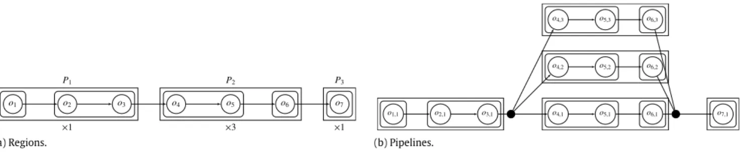
(a) Regions. (b) Pipelines.

Fig. 3. Regions and pipelines.

•

m

(

oi1,j

) =

m

(

oi2,j

) ⇒ ∀

l∈[1..r(o_i1)]

,

m

(

oi1,l

) =

m

(

oi2,l

)

. I.e, if

two operator replicas are assigned to the same thread, their sib-ling operator replicas should share their threads as well. For in-stance, if o1,1and o2,1both map to t1, then their siblings o1,2and

o2,2should share the same thread, say t2.

Regions and Pipelines. The above rules divide the program into

regions and these regions into sub-regions that we call pipelines, as

shown in the example inFig. 3.

In this example, we have 3 parallel regions: P1

= {

P1,1

,

P1,2

}

,

P2

= {

P2,1

,

P2,2

}

, and P3

= {

P3,1

}

. The first region P1has a single

replica, that is r

(

P1

) =

1 and it consists of two pipelines, namely

P1,1and P1,2. The first pipeline has a single operator inside, whereas

the second one has two operators. Concretely, we have P1,1

= {

o1

}

and P1,2

= {

o2

,

o3

}

. The second region has r

(

P2

) =

3, as there are

3 parallel channels, and it consists of 2 pipelines, namely P2,1and

P2,2. We have P2,1

= {

o4

,

o5

}

and P2,2

= {

o6

}

. Finally, the third

region is P3

= {

P3,1

}

, where r

(

P3

) =

1 and P3,1

= {

o7

}

.

Given the thread mapping function m and the replica function

r, the set of regions formed is denoted byP

(

m

,

r

)

orPfor short. To

find the first region, P1

∈

P, we start from the source operator o1

and locate the longest sequence of operators O′

_⊂

_{O s.t. o}

1

∈

O′

∧

(

Ls

(

O′

) ∨

Lp

(

O′

))

. We can apply this process successively, starting

from the next operator in line that is not part of the current set of regions, until the set of all regions,P, is formed. The pipelines for a given region are formed by grouping operators whose replicas for a parallel channel are assigned to the same thread by the mapping m. For each pipeline Pi,j

∈

Pi

∈

P, there are r

(

Pi

)

replicas and

a different thread executes each pipeline replica. Then the total number of threads used is given by



Pi∈Pr

(

Pi

)·|

Pi

|

. In the example

above, we have 9 threads and 13 operator replicas.

3.2. Modeling the throughput

Our goal is to define the throughput of a given configuration P. Once the throughput is formulated, we can cast our problem as an optimization one, where we aim to find the thread mapping function (m) and the operator replica counts (r) that maximize the throughput.

To formalize the throughput, we start with a set of helper definitions. We denote the kind of a region as k

(

Pi

)

, and define:

k

(

Pi

) =







f if

∃

ok

∈

Pi,j

∈

Pis.t. k

(

ok

) =

f s if

∀

_o_k∈Pi,j∈Pik

(

ok

) =

s p otherwise

.

(1)

For instance, inFig. 3, if o4and o6are stateless, and o5is

par-titioned stateful, then the parallel region P2becomes partitioned

stateful (p). As another example, if o2is stateful, then the region P1

becomes stateful.

We denote the selectivity of a pipeline Pi,j as s

(

Pi,j

) =



ok∈Pi,js

(

ok

)

, the selectivity of a region Pias s

(

Pi

) = 

Pi.j∈Pis

(

Pi,j

)

,

and the selectivity of the entire flowPas s

(

P

) = 

_P_i_∈Ps

(

Pi

)

. We

denote the cost of a pipeline as c

(

Pi,j

)

and define it as: c

(

Pi,j

) =



ok∈Pi,j

sk

(

Pi,j

) ·

c

(

ok

).

(2)

Here, sk

(

Pi,j

) = 

ol∈Pi,j,l<ks

(

ol

)

is the selectivity of the sub-pipeline

up to and excluding operator ok.

Region throughput. We first model a region’s throughput in isolation, assuming no other regions are present in the system. Let R

(

Pi

)

denote the maximum input throughput supported by a

region under this assumption. And let Rj

(

Pi

)

denote the output

throughput of the first j pipelines in the region assuming the remaining pipelines have zero cost. Furthermore, let R

(

Pi,j

)

denote

the input throughput of the pipeline Pi,jif all other pipelines had

zero cost (making it the bottleneck of the system). We have R0

(

Pi

) = ∞

and also for j

>

0: Rj

(

Pi

) =



s

(

Pi,j

) ·

Rj−1

(

Pi

)

if Rj−1

(

Pi

) <

R

(

Pi,j

)

s

(

Pi,j

) ·

R

(

Pi,j

)

otherwise

.

(3)

In essence, Eq.(3)models backpressure. If the input throughput of a pipeline, when considered alone, is higher than the output throughput of the sub-region formed by the pipelines before it, then the latter throughput is used to compute the pipeline’s output throughput when it is added to the sub-region. This represents the case when the pipeline in question is not the bottleneck. The other case is when the pipeline’s input throughput, when considered alone, is lower than the output throughput of the sub-region formed by the pipelines before it. In this case, the former throughput is used to compute the pipeline’s output throughput when it is added to the sub-region. This represents the case when the pipeline in question is the bottleneck within the sub-region. Modeling the backpressure is important, as most real-word data stream processing systems rely on it. As a concrete example, the lack of back-pressure in the popular open-source stream processing system Storm [36] has resulted in the development of Heron [29].

The throughput of a pipeline by itself, that is R

(

Pi,j

)

, can be

represented as:

R

(

Pi,j

) = (

c

(

Pi,j

) +

h

(

Pi,j

))

−1

,

(4)

where h

(

Pi,j

)

is the cost of switching threads between sub-regions,

defined as:

h

(

Pi,j

) = δ · (

1

(

j

>

1

) +

1

(

j

< |

Pi

|

) ·

s

(

Pi,j

)).

(5)

Here,

δ

is the thread switching overhead due to the queues involved in-between. The input overhead is incurred for the pipelines except the first one, and the output overhead is incurred for the pipelines except the last one.

With these definitions at hand, we can define the input through-put R

(

Pi

)

as the output throughput of the region divided by the

re-gion’s selectivity. That is:

(6)

Parallel region throughput. The next step is to compute the throughput of a parallel region. For that purpose, we first define an aggregate scalability function f

⟨

Pi

⟩

for the region Pias:

f

⟨

Pi

⟩

(

x

) =

min

ok∈Pi,j∈Pi

f

⟨

oi

⟩

(

x

).

(7)

The aggregate scalability function for a region simply takes the smallest scalability value from the scalability functions of the con-stituent operators within the region.

We denote the parallel throughput of a region Pias R∗

(

Pi

)

and

define it as follows: R∗

(

Pi

) =



cp

·

log2

(

r

(

Pi

)) +

1 R

(

Pi

) ·

f

⟨

Pi

⟩

(

r

(

Pi

))



−1

.

(8)

Here, cpis the replication cost factor for a parallel region. Recall

that a parallel region needs to reorder tuples. In the presence of selectivity, this often requires attaching sequence numbers to tuples and re-establishing order at the end of the parallel region. The re-establishment of order takes time that is logarithmic in the number of channels, per tuple. However, such processing typically has a low constant compared to the cost of the operators.

Let R+

(

Pi

)

be the parallel throughput of the region when it

is considered within the larger topology that contains the other regions, albeit assuming that all other regions have zero cost. We have: R+

(

Pi

) =



h

(

Pi

) +

1 R∗

(

_P i

)



−1

.

(9)

Here, h

(

Pi

)

is the cost of switching threads between regions,

which can be expressed as:

h

(

Pi

) = δ · (

1

(

i

>

1

) +

1

(

i

< |

P

|

) ·

s

(

Pi

)).

(10)

Throughput of a program. Given these definitions, we are ready to define the input throughput of a program, denoted as R

(

P

)

. We follow the same approach as we did for regions formed out of pipelines.

Let us define the output throughput of the first k regions as

Rk

(

P

)

, assuming the downstream regions have zero cost. We have R0

(

P

) = ∞

, and for i

>

0: Ri

(

P

) =



s

(

Pi

) ·

Ri−1

(

P

)

if Ri−1

(

P

) <

R+

(

Pi

)

s

(

Pi

) ·

R+

(

Pi

)

otherwise

.

(11) By dividing the output throughput of the program to its selec-tivity, we get:

R

(

P

) =

R|P|

(

P

)/

s

(

P

).

(12)

Bounded throughput. So far we have computed the unbounded throughput. In other words, we have assumed that each thread has a core available to itself. However, in practice, there could be more threads than the number of cores available. For instance, replicat-ing a region with 3 pipelines 3 times will result in 9 threads, but the system may only have 8 cores. However, replicating the region 2 times will result in an underutilized system that has only 6 threads and thus not all cores can be used.

Let C denote the number of cores in the system. We denote the bounded throughput of a program with parallelization config-uration of m (the thread mapping function) and r (the operator replica counts) as R

(

P

(

m

,

r

),

C

)

. The bounded throughput is sim-ply computed as the unbounded throughput divided by the

utiliza-tion times the number of cores. Formally,

R

(

P

,

C

) =

R

(

P

) ·

C

U

(

P

)

.

(13)

Here U

(

P

)

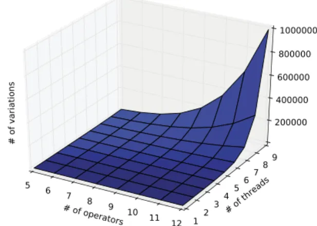
is the utilization for the unbounded throughput. Eq.(13)simply scales the unbounded throughput by multiplying

Fig. 4. # of parallel program configurations as a function of # of threads (M) and #

of operators (|O|).

it with the ratio of the maximum utilization that can be achieved (which is C ) to the unbounded utilization. We assume that the cost due to scheduling of threads by the operating system is negligible. For instance, if the unbounded throughput is 3 units, but results in a utilization value of 6 and the system has only 4 cores, then the bounded throughput is given by 3

· (

4

/

6

) =

2 units.

The computation of the utilization, U

(

P

)

, is straightforward. We already have a formula for the input throughput of the pro-gram, which can be used to compute the input throughputs of the parallel regions and the pipelines. Multiplying input throughputs of the pipelines with the pipeline costs would give us the utiliza-tion, after adding the overheads for the thread switching and scal-ability. Overall utilization can be expressed as:

U

(

P

) =

R

(

P

) ·



1≤i<|P| si

(

P

) · 

cp

·

log2

(

r

(

Pi

))

+

h

(

Pi

) +



1≤j<|Pi| sj

(

Pi

) · 

h

(

Pi,j

) +

c

(

Pi,j

).

(14)

Here, sj

(

Pi

) = 

1≤l<js

(

Pi,l

)

is the selectivity of the region Piup

to and excluding the jth pipeline, and sj

(

P

) = 

1≤l<js

(

Pl

)

is the

selectivity of the programPup to and excluding the jth region. Optimization. Our ultimate goal is to find argmax_m_,_rR

(P

(

m

,

r

),

C

)

, where m is subject to the rules we have outlined earlier. One way to solve this problem is to combinatorially generate all possible parallel configurations. This can be achieved via a recursive pro-cedure that takes the maximum number of threads M and the set of operators O as input, and generates all valid parallelization con-figurations of the operators that uses at most M threads. Let us denote the set of configurations generated by such a generator as

D

(

O

,

M

)

. Then we can compute argmax₍_m_,_r_)∈_D₍_O_,_M₎R

(

P

(

m

,

r

),

C

)

as the optimal configuration. There are two problems with this ap-proach. First, and the more fundamental one, is that, the computa-tion of D

(

O

,

M

)

takes a very long time even for a small number of threads and operators; and this time grows exponentially, since the number of variations increases exponentially (both with increasing number of operators and maximum number of threads).

Fig. 4shows the number of parallel configurations as a function of the number of operators and the maximum number of threads used. Second, we need to pick a reasonable value for M, which is typically greater than C . It can be taken as a constant times the number of cores, that is k

·

C . Unfortunately, using a large constant

will result in an excessively long running time for the configuration generation algorithm. On the other hand, using a small constant will have the risk of finding a sub-optimal solution.

(7)

Algorithm 1:PipelinedFission(O,M,α)

Data: O: operators (with their costs, c; selectivities, s; and state

kinds, k), M: number of cores,α: fusion cost threshold

Result: Pipelined fission configuration

R←ConfigureRegions(O, α) ◃Configure regions t←0;P←∅;r←∅ ◃Initialize best settings

for s∈0.1· [0..10]do ◃Range of utilization scalers P′_←

ConfigurePipelines(R,s·M) ◃Configure pipelines r′_←

ConfigureReplicas(R,P′_,_M₎ _◃_{Configure # of replicas}

t′_←

ComputeTput(R,P′,r′) ◃Compute the throughput

if t′_>_{t then t}_←_t′_;_P_←_P′_;_r_←_r′

return⟨R,P,r⟩ ◃Return the final configuration

4. Heuristic solution

In this section we present an algorithm to quickly solve the pipelined fission problem that was formalized in Section3. Our al-gorithm is heuristic in nature and trades off throughput optimality to achieve reasonable performance in terms of solution time. De-spite this, our results, presented later in Section5, show that not only does our algorithm achieve close to optimal throughput, but also it outperforms optimal versions of fission-only and pipelining-only alternatives.

4.1. Overview

Algorithm 1 presents our solution, which consists of three phases, namely (i) region configuration, (ii) pipeline configuration, and (iii) replica configuration. The region configuration phase di-vides the chain of operators into chains of regions. This is done based on the compatibility of the successive operators in terms of their state, while avoiding the creation of small regions that can-not achieve effective parallelization. The second and third phases are used to configure pipeline and data parallelism, respectively. That is, pipeline configuration creates pipelines within regions, and replica configuration determines the number of replicas for the re-gions. These two phases are run multiple times, each time with a different amount of CPU utilization reserved for them, but always summing up to the number of CPUs available in the system. In par-ticular, we range the fraction of the CPU utilization reserved for pipelining from 0% to 100%, in increments of 10%. The reason for running the pipeline and region configuration phases with differ-ing shares of CPU utilization is that, we do not know, a priori, how much parallelism is to be reserved for pipelining versus how much for fission, in order to achieve the best performance with respect to throughput. Among the multiple runs of the second and the third phases, we pick the one that gives the highest throughput as our final pipelined fission solution. Internally, pipeline configuration phase and replica configuration phase work similarly. In pipeline configuration, we repeatedly locate the bottleneck pipeline and divide it. In replica configuration, we repeatedly locate the bot-tleneck region and increase its replica count. In what follows, we further detail the three phases of the algorithm.

4.2. Region configuration

Algorithm 2 presents the region configuration phase, where we divide the chain of operators into a chain of regions. The algorithm consists of two parts. In the first part, we form effectively paral-lelizable regions. This may leave out some operators unassigned. In the second phase, we merge the consecutive unassigned opera-tors into regions as well.

The first for loop in Algorithm 2 represents the first step. We form regions by iterating over the operators. We keep accumulat-ing operators into the current region, as long as the operators are

Algorithm 2:ConfigureRegions(O,α)

Data: O: operators,α: fusion cost threshold

Result: Regions

R← {} ◃The list of regions that will hold the final result C ← {} ◃The list of operators in the current potential region

for i←1;i≤ |O|;i←i+1 do ◃For each operator ◃The current region borrows the operator’s properties

if k(oi) ̸=f∧(|C| =0∨k(C) =s)then

k(C) ←k(oi) ◃Update the region’s kind

if k(oi) =p then ◃If oiis partitioned

a(C) ←a(oi) ◃Update current region’s key

◃The current region stays partitioned, possibly with a broadened key

else if k(oi) =p∧a(oi) ⊆a(C)then

a(C) ←a(oi) ◃Update current region’s key

◃The current region and the operator are incompatible

else if k(oi) ̸=s then

if ComputeCost(C) > αthen ◃Region is costly enough R←R∪ {C} ◃Materialize the region in R d(o) ←1, ∀o∈C ◃Mark region’s operators as assigned

C← {} ◃Reset the current region

if k(oi) ̸=f then ◃Parallelizable operator

i←i−1 ◃Redo iteration with empty current region

continue

C←C∪ {oi} ◃Add the operator to the current region

◃Handle the pending region at loop exit

if ComputeCost(C) > αthen ◃Region is costly enough R←R∪ {C} ◃Materialize the region in R d(o) ←1, ∀o∈C ◃Mark region’s operators as assigned

◃Merge all consecutive unassigned ops to a region

C ← {} ◃Reset the current region

for i←1;i≤ |O|;i←i+1 do ◃For each operator

if d(oi) =1∧ |C|>0 then ◃We have a complete run

R←R∪ {C} ◃Materialize the region in R

C← {} ◃Reset the current region

else ◃Run of unassigned operators continues

C←C∪ {oi} ◃Add the operator to the current region

return R ◃The final set of regions

not stateful or incompatible. Stateless operators are always com-patible with the current region. Partitioned stateful operators are only compatible if their key is the same as the key of the active re-gion so far, or broader (has less attributes). In the latter case, the region’s key is updated accordingly. When an incompatible opera-tor is encountered, the current region that is formed so far is com-pleted. However, this region is discarded if its overall cost is below the fusion cost threshold,

α

. The motivation behind this is that, if a region is too small in terms of its cost, parallelization overhead will dominate and effective parallelization is not attainable.

Once a region is completed, the algorithm continues with a fresh region, starting from the next operator in line (the one that ended the formation of the former region). The first step of the algorithm ends, when all operators are processed. In the second step, the operators that are left without a region assignment are handled. Such operators are either stateful or cannot form a sufficiently costly region with the other operators around them. In the second step, consecutive operators that are not assigned a region are put into their own region. However, these regions cannot benefit from parallelization in the pipeline and replica configuration phases that are described next.

4.3. Pipeline configuration

Algorithm 3 describes the pipeline configuration phase. We start with each region being a pipeline and iteratively split

(8)

Algorithm 3:ConfigurePipelines(R,M)

Data: R: regions, M: number of cores Result: Pipeline configuration

P←R ◃Initialize the set of pipelines to regions ◃Find the bottleneck pipeline (C ), and compute the total utilization

(U)

⟨C,U⟩ ←FindBottleneckPipeline(R,P)

while U≤M do ◃System is not fully utilized ◃Find the best split for the pipeline (maximizes throughput) oi←argmaxok∈CComputeTput({oj∈C|j<k}, {oj∈C|j≥k})

C0← {oj∈C|j<i} ◃First half of the best split

C1← {oj∈C|j≥i} ◃Second half of the best split

if ComputeTput({C0,C1}) ≤ComputeTput(C)then

break ◃No further improvement is possible P←P\ {C} ∪ {C0,C1} ◃Split the pipeline

⟨C,U⟩ ←FindBottleneckPipeline(P) ◃Re-eval. for next iter.

return P ◃The final set of pipelines

Algorithm 4:ConfigureReplicas(R,P,M)

Data: R: regions, P: pipelines, M: number of cores Result: Set of number of replicas of each region

r[C] ←1, ∀C∈R ◃Initialize the replica counts to 1

◃Find the bottleneck region (C ), and compute the total utilization (U)

⟨C,U⟩ ←FindBottleneckRegion(R,P,r)

while U≤M do ◃System is not fully utilized t←_{CalculateTput}(R,P,r) ◃Baseline throughput r[C] ←r[C] +1 ◃Increase the channel count

if t≥CalculateTput(R,P,r)then ◃Throughput decreased

r[C] ←r[C] −1 ◃Revert back

break ◃No further improvement is possible ⟨C,U⟩ ←FindBottleneckRegion(R,P) ◃Re-eval. for next iter.

return r ◃Return the replica counts

the bottleneck pipeline. The FindBottleneckPipeline procedure is used to find the bottleneck pipeline. This procedure simply computes the unbounded throughput of the program as new pipelines are successively added, using the formalization from Section3, and selects the last pipeline that resulted in a reduction in the unbounded throughput as the bottleneck one. It then reports this bottleneck pipeline, together with the utilization of the current configuration. If the utilization is above or equal to the total utilization reserved for the pipeline configuration phase (recall Algorithm 1), then the iteration is terminated and the pipeline configuration phase is over. Otherwise, i.e., if there is room available for an additional pipeline, we find the best split within the bottleneck pipeline. This is done by considering each operator as a split point and picking the split that provides the highest unbounded throughput. However, if the unbounded throughput of this split configuration of two consecutive pipelines is lower compared to the original single pipeline (which might happen for low cost pipelines due to the impact of thread switching overhead), we again terminate the pipeline configuration phase. This is because, if the bottleneck pipeline cannot be improved, then no overall improvement is possible.

4.4. Replica configuration

Algorithm 4 describes the replica configuration phase. It is sim-ilar in structure to the pipeline configuration phase. However, it works on regions, rather than pipelines. It iteratively finds the bot-tleneck region and increases its replica count. The FindBottle-neckRegion procedure is used to find the bottleneck region. This

procedure simply computes the unbounded throughput of the pro-gram as new regions are successively added, using the formaliza-tion from Secformaliza-tion3, and selects the last region that resulted in a reduction in the unbounded throughput as the bottleneck one. It then reports this bottleneck region, together with the utilization of the current configuration. If the utilization is above the number of CPUs available, then the iteration is terminated and the replica con-figuration phase is over. Otherwise, i.e., if there is room available for an additional parallel channel, we increment the replica count of the bottleneck region. However, if the unbounded throughput of this parallel region with an incremented replica count has a lower unbounded throughput compared to the original parallel region (which might happen for low cost regions due to the impact of replication cost factor and thread switching overhead), we again terminate the region configuration phase. This is because if the bot-tleneck region cannot be improved, then no overall improvement is possible.

5. Evaluation

In this section, we evaluate our heuristic solution and showcase its performance in terms of the achieved throughput, as well as the time it takes to locate a parallelization configuration. We perform two kinds of experiments. First, we evaluate our pipelined fission solution using model-based experiments under varying workload and system settings. Second, we evaluate our algorithm using stream programs written in IBM’s SPL language [20] and executed using the IBM InfoSphere Streams [12] runtime.

In our experiments, we compare our solution against four different approaches, namely: optimal, sequential, fission-only, and pipelining-only.

•

Sequential solution is the configuration with no parallelism.

•

Optimal solution is the configuration that achieves the

maxi-mum throughput among all possible parallel configurations.

•

Fission-only optimal solution is the configuration that achieves

the highest throughput among all possible parallel configura-tions that do not involve pipeline parallelism (that is, each par-allel channel is executed by a single thread).

•

Pipelining-only optimal solution is the configuration with the

highest throughput among all possible parallel configurations that do not involve data parallelism.

5.1. Experimental setup

For the model-based experiments, we used the analytical model presented in Section3to compare alternative solutions. The five alternative solutions we study were all implemented in Java. The SPL experiments rely on the parallelization configurations generated by these solutions to customize the runtime execution of the SPL programs. The SPL programs are compiled down to C++ and executed on the Streams runtime [12].

We describe the experimental setup for the model based ex-periments inTable 1. Each model based experiment was repeated 1000 times, whereas SPL based experiments were repeated 50 times. All experiments were executed on a Linux system with 2 Intel Xeon E5520 2.27 GHz CPUs with a total of 12 cores and 48 GB of RAM.

We discuss the thread switching overhead and replication cost factor for the SPL experiments later in Section5.3.

5.2. Model-based experiments

Streaming applications contain operators with diverse prop-erties. Accordingly, the throughput of the topology is highly de-pendent on the properties of the operators involved. Hence, we evaluate our solution by varying operator selectivity, operator

(9)

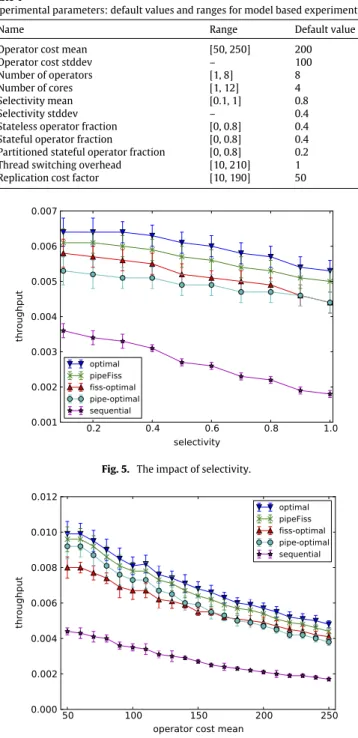
Table 1

Experimental parameters: default values and ranges for model based experiments.

Name Range Default value

Operator cost mean [50, 250] 200

Operator cost stddev – 100

Number of operators [1, 8] 8

Number of cores [1, 12] 4

Selectivity mean [0.1, 1] 0.8

Selectivity stddev – 0.4

Stateless operator fraction [0, 0.8] 0.4

Stateful operator fraction [0, 0.8] 0.4

Partitioned stateful operator fraction [0, 0.8] 0.2

Thread switching overhead [10, 210] 1

Replication cost factor [10, 190] 50

Fig. 5. The impact of selectivity.

Fig. 6. The impact of operator cost.

cost, and operator kind with respect to state. Our default settings use an operator cost that is 200 times the thread switching over-head. When projected on SPL, this corresponds to a per-tuple op-erator cost of 19

µ

s, which is quite reasonable based on our obser-vation of real-world operator costs (seeFig. 17for a sample real-world application and its operator costs). In addition, a variety of other factors impact the throughput of the topology, among which four most important ones are replication cost factor, thread switch-ing overhead, number of cores, and the number of operators. Ac-cordingly, we also perform experiments on these.

5.2.1. Operator selectivity

The impact of operator selectivity on the performance of our solution is shown in Fig. 5. The figure plots the throughput (y-axis) as a function of the mean operator selectivity (x-axis)

Fig. 7. The impact of the operator kind.

for different approaches. We observe that for the entire range of selectivity values, our solution outperforms the fission-only and pipelining-only optimal approaches, and provides up to 2.7 times speedup in throughput compared to the sequential approach. The throughput provided by our approach is also consistent within 5% of the optimal solution, for the entire range of selectivity values. Interestingly, we observe that the pipelining-only approach provides reduced performance compared to fission-only approach, for low selectivity values. This is because with reducing selectivity, the performance impact of the operators that are deeper in the pipeline reduces, which takes away the ability of pipelining to increase the throughput (as speedup due to pipelining is limited by the pipeline depth).

5.2.2. Operator cost mean

The impact of operator cost on the performance of our solution is shown inFig. 6. The figure plots the throughput (y-axis) as a func-tion of the mean operator cost (x-axis) for different approaches. Again we observe that the pipelined fission solution is quite ro-bust, consistently outperforming fission-only and pipelining-only optimal solutions, and staying within 5% of the optimal solution. It achieves up to 2.5 times speedup in throughput compared to the sequential approach. One interesting observation is that, for smaller mean operator cost values, the performance of the fission-only approach is below the pipelining-fission-only approach, but gradu-ally increases and passes it as the mean operator cost increases. The reason is that, the fission optimization has a higher overhead due to the replication cost factor, and thus, for small operator costs, it is not beneficial to apply fission. As the operator cost increases, fission becomes more effective.

5.2.3. Operator kind

The impact of the operator kind on the performance of our solution is shown inFig. 7. Recall that operators can be stateful, stateless, or partitioned stateful. Fig. 7 plots the throughput (y-axis) as a function of the fraction of stateless operators (x-axis) for different approaches. While doing this, we keep the fraction of partitioned stateful operators fixed at 0.2. We observe that the percentage of stateless operators do not impact the pipelining-only solution. The reason is that pipeline parallelism is applicable for both stateful and stateless operators. On the other hand, fission-only solution improves as the percent of the stateless operator increases. The reason is that data parallelism is not applicable for stateful operators. We also observe that our pipelined fission solution stays close to the optimal throughout the entire range of the stateless operator fraction. Again, pipelined fission clearly outperforms pipelining-only and fission-only approaches.

(10)

Fig. 8. The impact of replication cost factor.

Fig. 9. The impact of the thread switching overhead.

5.2.4. Replication cost factor

The impact of the replication cost factor on the performance of our solution is shown inFig. 8. The figure plots the throughput (y-axis) as a function of the replication cost factor (x-axis) for dif-ferent approaches. The results indicate that our solution consid-erably outperforms pipelining-only and fission-only approaches, providing up to 25% higher throughput compared to pipelining-only optimal approach and up to 30% higher throughput compared to fission-only optimal approach. Note that our pipelined fission approach provides performance as good as fission-only optimal ap-proach when the replication cost factor is close to 0 and as good as pipelining-only optimal approach when the replication cost factor is very high. In effect, our solution switches from using fission to using pipelining as the replication cost factor increases. We also observe that the optimal solution’s throughput advantage is big-ger for small replication cost factors, yet the gap with pipelined fission quickly closes as the replication cost factor increases. In the SPL based experiments presented later, we show that for realistic replication cost factors, our solution provides performance that is very close to the optimal.

5.2.5. Thread switching overhead

The impact of the thread switching overhead on the perfor-mance of our solution is shown inFig. 9. The figure plots the throughput (y-axis) as a function of the thread switching overhead (x-axis) for different approaches. We observe that the throughput of all solutions, except the sequential one, decreases as the thread switching overhead increases. It is an expected result as all so-lutions benefit from parallelism via using threads, except the se-quential solution. Again, our pipelined fission solution outperforms

Fig. 10. The impact of the number of cores.

Fig. 11. The impact of the number of operators.

pipelining-only and fission-only optimal solutions, and is able to stay close to the optimal performance throughout the entire range of thread switching overhead values. We also observe that as the thread switching overhead increases, all approaches start to get closer in terms of the throughput. This is due to the reducing paral-lelization opportunities, as a direct consequence of the high thread switching overhead values.

5.2.6. Number of cores

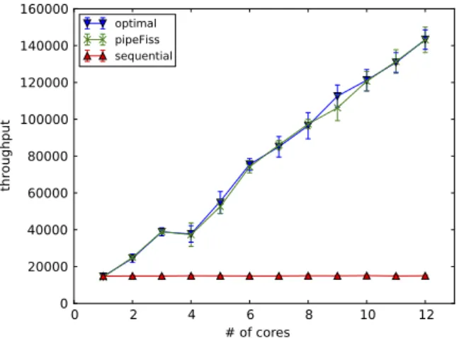
The impact of the number of cores on the performance of our solution is shown inFig. 10. The figure plots the throughput (y-axis) as a function of the number of cores (x-axis) for different approaches. We observe that for all approaches, the throughput only increases to a certain degree, after which it stays flat. There are two reasons for not being able to achieve linear speedup: (i) not all operators are parallelizable, (ii) the thread switching and replication cost factor introduce overheads in parallelization. We again observe that our pipelined fission approach outperforms the pipelining-only and fission-only optimal solutions. With increasing number of cores, the gap between the optimal approach and alternatives increases, as the search space gets bigger. However, since the throughput flattens quickly, the increase in the gap eventually stops. At that point, our approach is still within 8% of the optimal.

5.2.7. Number of operators

The impact of the number of operators on the performance of our solution is shown inFig. 11. The figure plots the throughput (y-axis) as a function of the number of operators (x-axis) for

(11)

Fig. 12. Running time (in milliseconds).

different approaches. We observe that as the number of operators increases, the performance of the pipelining-only solution relative to the fission-only solution increases. The reason is that the pipeline parallelism cannot help a single operator, so it is not as effective for small number of operators. Our pipelined fission solution provides up to 18% higher throughput compared to the closest alternative. While the gap between the optimal solution and ours increases with increasing number of operators, eventually throughput flattens due to the fixed number of cores available. Importantly, our approach stays within 5% of the optimal solution.

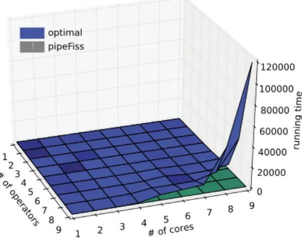
5.2.8. Running time

We also evaluate the running time of our pipelined fission algorithm. Fig. 12 plots running time in terms of milliseconds, for our pipelined fission solution and the exhaustive optimal approach. Unfortunately, the running time of the optimal solution dramatically increases with increasing number of operators and cores. For 9 operators and 9 cores, the running time reaches 2 min, which makes it inapplicable for runtime adaptation. Furthermore, the time grows very quickly, reaching hours for 10 operators and 10 cores (not shown), and becomes practically unusable even for static optimization for larger setups. However, even if the number of operators and cores are high, our pipelined fission algorithm completes much faster (under 5 ms).

5.3. SPL experiments

In our second set of experiments, we use IBMs SPL language and its InfoSphere Streams runtime to evaluate the effectiveness of our solution. In order to perform this experiment, we need to determine the value of the replication cost factor and the thread switching overhead for the InfoSphere Streams runtime.

5.3.1. Thread switching overhead

For determining the thread switching overhead, we use a simple pipeline of two operators. We run this topology twice, once with a single thread and again with two threads. Let c be the cost of the operator. For the case of two threads, the throughput achieved, denoted as Tp, is given by:

Tp

=

1

/(

c

+

δ).

(15)

On the other hand, for the case of a single thread, the throughout achieved, denoted as Ts, is given by:

Ts

=

1

/(

2

·

c

).

(16)

By using Ts and Tp, we can compute the thread switching

overhead,

δ

, without needing to know the operator cost c. More specifically,

δ =

1 Tp

−

1 2

·

Ts

.

(17)

In order to calculate the thread switching overhead for our SPL experiments, we measure the throughput of the topology with and without pipeline parallelism for varying tuple sizes, and use Eq.(17)to compute the thread switching overhead. The use of different tuple sizes is due to the implementation of thread switching within the SPL runtime, which requires a tuple copy (the cost of which depends on the tuple size).

5.3.2. Replication cost factor

For determining the replication cost factor, we use a simple pipeline of three operators, where the first and the last operators are the source and the sink operators with no work performed and the middle operator has cost c. We then run this topology with different number of parallel channels used for the middle operator. Let n denote the number of channels used. We can formulate the throughput as: Tp

(

n

) =



2

· δ +

c n

+

log2n

·

cp



−1

.

(18)

If we know the throughput for two different number of channels, say T

(

n1

)

and T

(

n2

)

, then we can compute the replication

cost factor, cp, independent of other factors, such as the cost c, as

follows: cp

=

1 n2·Tp(n1)

−

1 n1·Tp(n2) log2n1 n2

−

log2n2 n1

.

(19)

In order to calculate the replication cost factor for our SPL experiments, we measure the throughput of our sample topology with different number of replicas for varying tuple sizes, and use Eq.(19)to compute the replication cost factor.

By using the calculated thread switching overhead and repli-cation cost factor values, we perform SPL experiments to evaluate our solution for varying operator count, selectivity, cost, and kind. Throughput is again our main metric for evaluation. The applica-tions used for these experiments are similar to the ones from the model-based experiments, but are written using the SPL language. The operators used are busy operators that perform repeated mul-tiplication operations to emulate work (the cost is the number of multiplications performed). To emulate selectivity, they draw a random number for each incoming tuple and compare it to the selectivity value to determine if the tuple should be forwarded or not. This setup enables us to study a wide range of parameter set-tings. To further strengthen the evaluation, we have also applied our pipelined fission solution to a real-world application called

LogWatch, which we detail later in this section. 5.3.3. Operator selectivity

Fig. 13 plots throughput (y-axis) as a function of the mean operator selectivity (x-axis) for the optimal, pipelined fission, and sequential solutions using SPL. We see that all approaches achieve lower throughput as the operator selectivity increases. Pipelined fission solution provides practically the same performance as the optimal solution for selectivities beyond 0.7 and is within 15% of the optimal for selectivities as small as 0.3. When the selectivity gets very low, the variance in results significantly increases as very few tuples make it through the pipeline.