Extended phase diagram of ASEP with two types of particles

EXTENDED PHASE DIAGRAM OF ASEP

WITH TWO TYPES OF PARTICLES

a thesis

submitted to the department of physics

and the institute of engineering and science

of bilkent university

in partial fulfillment of the requirements

for the degree of

master of science

By

Ay¸se Ferhan Ye¸sil

December, 2010

I certify that I have read this thesis and that in my opinion it is fully adequate, in scope and in quality, as a thesis for the degree of Master of Science.

Prof. Dr. M. Cemal Yalabık (Advisor)

I certify that I have read this thesis and that in my opinion it is fully adequate, in scope and in quality, as a thesis for the degree of Master of Science.

Prof. Dr. Bilal Tanatar

I certify that I have read this thesis and that in my opinion it is fully adequate, in scope and in quality, as a thesis for the degree of Master of Science.

Assoc. Prof. Dr. Azer Kerimov

Approved for the Institute of Engineering and Science:

Prof. Dr. Levent Onural Director of the Institute

ABSTRACT

EXTENDED PHASE DIAGRAM OF ASEP WITH TWO

TYPES OF PARTICLES

Ay¸se Ferhan Ye¸sil M.S. in PHYSICS

Supervisor: Prof. Dr. M. Cemal Yalabık December, 2010

The ASEP (Asymmetric Simple Exclusion Process) model system with two types of particles is studied. The system is interesting because it exhibits spontaneous symmetry breaking when parameters controlling the dynamics of the two types of particles of the same system. By using Mean Field approximation its extended phase diagram was obtained for non-symmetric values of entering rates of the two types of particles. The system is understood to be the combination of two decoupled ASEP systems with one type of particle system for the values of equal hopping and exchange rates. (Evans et al.,PR E, 74 208, (1995)) It is understood that for the exchange rates different from the hopping rates the system can no longer be analyzed as combination of two decoupled one particle ASEP. The “tiny phase” first observed by Evans et al, is examined in more detail. It is found that this phase still exists when entering rates are not symmetric. Also, Monte Carlo simulations for certain values of parameters of the system were carried out to determine the particle density profiles. The phase diagram of the system displays unexpectedly rich structure for the relatively simple dynamics.

Keywords: ASEP, spontaneous symmetry breaking, phase diagram, non-equilibrium, steady state.

¨

OZET

˙IK˙I PARC¸ACIKLI ASEP MODEL˙IN˙IN GEN˙IS¸LET˙ILM˙IS¸

FAZ D˙IYAGRAMI

Ay¸se Ferhan Ye¸sil

F˙IZ˙IK, Y¨uksek Lisans

Tez Y¨oneticisi: Prof. Dr. M. Cemal Yalabık Aralık, 2010

Bu ¸calı¸smada iki t¨ur par¸cacık i¸ceren ABDS (Asimetrik Basit Dı¸slama S¨ureci)

model sistemi incelendi. Sistem, iki t¨ur par¸cacı˘gın dinami˘gini kontrol eden

parametrelerin aynı oldu˘gu durumda kendili˘ginden simetri kırılması g¨osterdi˘gi

i¸cin ilgi ¸cekmekte. Ortalama alan yakınla¸stırması kullanılarak sistemdeki iki t¨ur

par¸cacı˘gın giri¸s olasılıksal hızlarının simetrik olmadı˘gı durum icin genelle¸stirilmi¸s faz diyagramı elde edildi. E¸sit yer de˘gi¸sme ve zıplama olasılıksal hızları i¸cin sis-temin iki ayrı tek par¸cacıklı ABDS’nin birle¸simi oldu˘gu bilinmektedir (Evans ve

ark., PR E, 74 208, (1995)). Yer de˘gi¸sme olasılıksal hızları ile zıplama hızlarının

aynı olmadı˘gı durumlarda sistemin artık iki ayrı tek par¸cacıklı ABDS olarak ince-lenemeyece˘gi anla¸sıldı. Evans ve ark. tarafından ilk kez g¨ozlenen “ince faz”ın giri¸s olasılıksal hızların e¸sit olmadı˘gı zamanlarda da var oldu˘gu g¨ozlemlendi. Par¸cacık yo˘gunluk da˘gılımlarının bulunması i¸cin belli parametre de˘gerleri i¸cin Monte Carlo benzetimleri yapıldı. Sistemin faz diyagramı, g¨orece basit olan dinamiklerine

kıyasla beklenmedik ¨ol¸c¨ude zengin yapı g¨osterdi.

Anahtar s¨ozc¨ukler: ASEP, faz diyagramı, kendili˘ginden simetri kırılması, dengede olmayan, dura˘gan durum.

v

Acknowledgement

I am heartily thankful to Prof. Dr. M. Cemal Yalabık for his generousity in sharing his enthusiasm, vast knowledge and experience with me. He has not just thaught me physics and coding, he also thaught me how to cope with problems of real life. I’m also very much impressed and inspired by his enthusiasm and meticulous care about teaching and advising new scientists.

I also would like to express my grattitude to Prof. Dr. Ne¸se Yalabık for letting me know her inspiring character as a succesful scientist, a dedicated teacher and a caring mother.

I am also indebted to Prof. Dr. Bilal Tanatar, Assoc. Prof. Azer Kerimov for their time and interest in reading and reviewing this thesis and also giving me the exciting physics and mathematics lectures that I have learned a lot.

Also, I would like to thank to M.Sc. Ba¸sak Renklio˘glu, Asst. Prof. Levent Suba¸sı and M.Sc. Ertu˘grul Karademir for fruitful discussions on the subject matter and their technical support.

I am also thankful to T ¨UBA for supporting my participation in 17. IFG and

2. Turkish-Greek Meeting.

I would like to thank to Bet¨ul G¨urzel, Merve Tanık, Semih C¸ akmakyapan who

listened and and supported me with their appearance in my thesis defense. I also would like to add special thanks to all my colleagues in Bilkent Physics Department with whom I spent nice time during and after work.

Lastly, I want to say this thesis would not have been possible unless my father

M¨ukerrem Ye¸sil, my mother Ya¸sag¨ul Ye¸sil and my sister ˙Ilay Ye¸sil did not show

me their warm support and kind tolerances.

Contents

2.2 ASEP with one type of particle . . . 5

2.3 ASEP with two types of particles . . . 8

3 Methods of Analysis 10 3.1 Matrix Product Method . . . 11

3.2 Mean Field Theory . . . 12

3.2.1 Present Work . . . 13

3.3 Renormalization Group Theory . . . 14

3.4 Monte Carlo Method . . . 15

CONTENTS _viii

4 Results 16

4.1 Mean Field Approximation . . . 16

4.2 Monte Carlo Simulation . . . 23

5 Conclusion and Future Work 24

List of Figures

1.1 The detailed balance and the steady state are shown

schemati-cally, choosing different line styles in the second figure indicates the probability flow for going from one state to another state is

not equal to the flow for the reverse process. . . 2

1.2 Transition between liquid and gas phases as a function of pressure

and time. The point (Tc, Pc) is the critical point. . . 3

2.1 Schematic display of ASEP with one type of particle. . . 5

2.2 Exact phase diagram for one type of particle ASEP system. The

dotted line shows the first order transition. . . 5

2.3 Exact renormalization phase diagram of ASEP system with one

type of particle, adapted from Georgiev et al.’s graph [10]. . . . . 6

2.4 Phase diagram of approximate renormalization group solution to

ASEP system with one type of particle, adapted from the work of

Hanney et al. [11]. . . . 7

2.5 Schematic display of ASEP with two types of particles. . . 8

2.6 This is the phase diagram of ASEP with two classes of particles,

adapted from the phase diagram found by Evans et al.[3] . . . . . 9

LIST OF FIGURES _x

4.1 Phase diagram of ASEP with two types of particles as function of

α2, for the case α1 = γ1 = γ2 = δ = 1. . . 17

4.2 The phase diagram obtained through MF for β = β1 = β2 and

γ1 = γ2 = δ = 1. The line where metastability can be observed is

also added to the Fig. 4.1 . . . 18

4.3 First order hysteresis curves for density. Hysteresis indicates the

double-valuedness of density for small values of β. . . 19

4.4 The tiny phase, where the symmetry starts to be broken but the

difference of the values of states are close to each other. ∆β

indi-cates the β width of the phase. . . 20

4.5 ∆β vs α both drawn on logarithmic scale. Here the ∆β is the

width in Fig.4.4 . . . 21

4.6 3-D graph of current changes, first order changes are indicated

by discontinuities in the lines. Here the currents are also double-valued for small values of β , however it is cut off to show how the

current values jump. . . 21

4.7 The current difference graph for some values of δ. It is seen that

for values bigger than δ = 1, current values exceed the maximum

value 0.25 . . . 22

4.8 Behavior of tiny phase for different values of δ. The tiny phase

does not exist for values δ < 0.8 . . . 22

4.9 Some density profiles of the phases as density vs site of the chain.

The order of the density profiles from left to right MM, ML, HL,

List of Tables

2.1 The density and current expressions for each phases of ASEP with

one type of particle. . . 6

Chapter 1

Introduction

Equilibrium systems have been studied extensively since the work of Gibbs[1] and Boltzmann[2]. However nonequilibirum systems are not that well-understood, al-though they are very common in nature.

In this thesis, a non-equilibrium model is studied. The model is chosen since although it is a relatively simple model it shows interesting characteristics of

non-equilibrium systems. In steady state, it has a symmetry broken phase

transition[3]. In some versions of the model avalanches and shock profiles are also observed[4]. On the other hand the model can be applied to real life problems, such as traffic flow[5], inter-cellular transportation[6] and bio-polymerization[7]. To study the model Mean Field and Monte Carlo methods are applied. Extended phase diagram of the system has been found.

1.1

Equilibrium

Equilibrium in this context, is the probabilistic equilibrium. Nonequilibrium is the lack of this probabilistic equilibrium and steady state is a special case of the non-equilibrium state. To be more precise, in equilibrium probabilities are not changing with time, and in addition the rate of probability flow for changing from one state to another is equal to the flow for coming back to the previous

CHAPTER 1. INTRODUCTION ₂

state. Probability flow is related to the change of the probability of a state. Since

total probability is conserved the quantity Piwi→j (where Pi is the probability

of i’th configuration and wi→j is the rate of change of i’th configuration to the

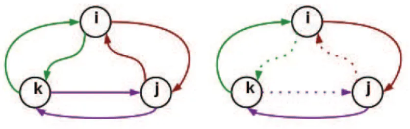
j’th configuration) gives the probability flow from state i to j. This property is known as detailed balance. In this sense the non-equilibrium state is the state where probabilities are changing with time or when there is no detailed balance in the probability among states. A special case of the non-equilibrium state is the steady state which is a state when probabilities are not changing with time as in the equilibrium case but there are currents in the system. These currents can be energy currents, particle density currents etc. Fig. 1.1 shows the schematic explanation for detailed balance and steady state.

Figure 1.1: The detailed balance and the steady state are shown schematically, choosing different line styles in the second figure indicates the probability flow for going from one state to another state is not equal to the flow for the reverse process.

1.2

Phase Transitions

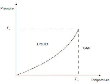
Phase transition is a non-analytic behavior in some macroscopic average quantity as a function of some controllable parameter. This macroscopic quantity can be a thermodynamic quantity such as pressure, density or current. For example in Fig. 1.2 one can see that there are two kinds of possible changes from liquid to gas. One type of change is by crossing the line, and the other one is by turning around that line. Here the phase transition through the line is first order transition, because the density changes discontinuously. However there is no phase transition when turning around the line. Because the density changes continuously, one can see

CHAPTER 1. INTRODUCTION ₃

that the liquid and the gas have similar type of structure. The derivative of the

density changes discontinuously, when one goes through the critical point (Tc, Pc),

which is a second order transition.

Figure 1.2: Transition between liquid and gas phases as a function of pressure

Chapter 2

The Model

2.1

ASEP

Asymmetric Simple Exclusion Process (ASEP) is a one dimensional, open-ended chain model, where particles join into the system from one end, hop to empty sites and jump out of the other end of the system by certain corresponding rates. This kind of processes are also known as “boundary-driven open diffusive system” or “open driven diffusive system” in literature. A special case of this model is Totally Asymmetric Simple Exclusion Process (TASEP) where the particles are allowed to hop only in a certain direction. However most of the papers and also in this thesis TASEP are called ASEP. ASEP is a limit of Katz-Lebowitz-Spohn (KLS) model[8]. KLS model is a two-dimensional lattice model, where particles are allowed to hop forwards, backwards, up and down. The ASEP limit is reached by taking the effective field as infinite which allows hops for only a certain direction.

CHAPTER 2. THE MODEL ₅

2.2

ASEP with one type of particle

In ASEP with one type of particle, particles enter the system from one end in time dt with probability αdt, go out from the system with probability βdt and hop into empty sites with probability γdt.

Figure 2.1: Schematic display of ASEP with one type of particle.

This problem is exactly solvable. It can be solved by the matrix product

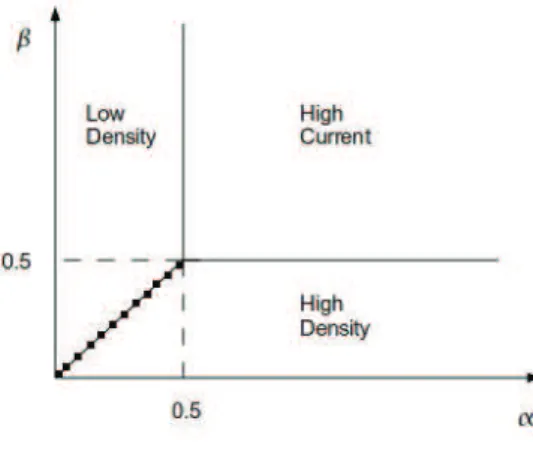
method[9]. Other methods such as exact[10] and approximate[11] renormalization group analysis have also been used. The resulting phase diagram of the system has a relatively simple form. In the region where α is bigger than β, with β less than 0.5 the system is in high density state. In the region where β is bigger than α, and α is at most 0.5 the system is in low density phase. Moreover, if both the values of α and β are bigger then the critical value 0.5, the system is in the maximal current phase. Here high rates cause particles to enter and leave the system more frequently. The exact solution yields the following values for current

Figure 2.2: Exact phase diagram for one type of particle ASEP system. The dotted line shows the first order transition.

CHAPTER 2. THE MODEL ₆

and density:

Phase Current Density

Low Density α(1 − α) α High Density β(1 − β) 1 − β High Current 1 4 1 2

Table 2.1: The density and current expressions for each phases of ASEP with one type of particle.

As can be seen from the table I the change in density when one goes from the low density to high density is discontinuous, however all other changes are contin-uous combined with the discontinuities in higher order derivatives. Discontinuity means the transition is first order while continuity means it is second order. The exact renormalization group study of Georgiev et al., implements renormal-ization of the matrix product method[10]. The RG method is described in section 3.3 of this thesis. Their analysis produces the exact phase transition structure which can be seen in Fig.2.3.

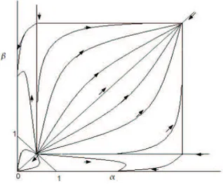
Figure 2.3: Exact renormalization phase diagram of ASEP system with one type of particle, adapted from Georgiev et al.’s graph [10].

In Fig. 2.3 fixed points are shown at points (α, β) equal to (0,0), (0,1), (1,0), (0.5,0.5), (2.929,2.929), (0.5, 2.929) and (2.929, 0.5). The trivial solution of the matrix product method at the line α + β = 1 is also emphasized by phase flow in

CHAPTER 2. THE MODEL ₇

the graph. In the approximate renormalization approach of Hanney et al. they map six-sited ASEP chain to two-sited chain, for a scale factor b = 3 by using matrix product method. Note that this approach would give the exact values if the chain size was infinite but that would mean solving the problem exactly. Since in this work chain size is finite the phase diagram in Fig. 2.4 is somewhat dif-ferent from the exact diagram. Here in Fig.2.4, the capital letters A-G represent

Figure 2.4: Phase diagram of approximate renormalization group solution to ASEP system with one type of particle, adapted from the work of Hanney et al. [11].

the fixed points. These fixed points characterize either the phase separatrixes or the phases. The points A through D correspond to exact values while points E through G would approach exact values when chain size becomes very large. The lines with arrows between these points show the RG flow and the arrows show the direction of this flow. Here A is an unstable fixed point which is found to have

the values ρc=

1

2 and Jc=

1

4. Points B, C and D are zero-current fixed points. And

CHAPTER 2. THE MODEL ₈

2.3

ASEP with two types of particles

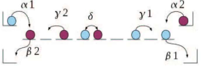
In this thesis we study ASEP with two types of particles. (Fig. 2.5) Here each type of particle can go in one direction which is opposite to the other one. Par-ticles can hop to a site in one direction if it is empty and whenever they meet head to head with a different type of particle they can exchange their sites with rate δ.

Figure 2.5: Schematic display of ASEP with two types of particles.

This system has no exact solution. Matrix product method has not been success-ful in obtaining a solution to this problem[9]. Since then, Evans et al. has applied the mean field approximation on the master equation of this system. They look

at the special case α1 = α2, β1 = β2 and γ1 = γ2 = δ and also scale the time

of the system by taking δ = 1. They found the unexpected result that below

β1 = β2 = 0.333 and α1 = α2 = 1 the system goes into spontaneous symmetry

breaking. In this state the system begins to favor one type of the particles al-though the parameters for both types are the same. Also they found a special phase existing in a very small region of the phase diagram. The phase diagram of this model can be seen in Fig. 2.6.

In the phase diagram of Evans there are four phases, two of them are sym-metric in values of density and currents of the two types of particles while the other two have broken symmetries. Symmetric ones are msximal current (MC), low density (LD) phases, while symmetry-broken phases are low density-low den-sity (LD-LD) and high denden-sity-low denden-sity (HD-LD) phases. Here the origi-nal notation used in the paper of Evans et al. has been used. They used the

phase1 −phase2 notation if the currents of the two types of particles are not

CHAPTER 2. THE MODEL ₉

Figure 2.6: This is the phase diagram of ASEP with two classes of particles, adapted from the phase diagram found by Evans et al.[3]

Chapter 3

Methods of Analysis

For a large number of many-body problems, exact solutions do not exist. Mas-ter equation is the equation which describes how the probabilities change with

respect to time. In mathematical representation d

dtP = LP , where P is vector of

the probability values and L is the Liouville matrix whose elements are rates of changes. As it is defined before, steady state is characterized with time invariant

probabilities. Then this implies d

dtPss= 0 which is the condition for steady state.

Now one has to solve this Lu = 0 equation. Here u is the steady state probabil-ity distribution which corresponds to a zero-eigenvalue eigenvector. The system ending in spontaneous symmetry breaking suggests that there may be degeneracy in the Liouville matrix for the model. In other words there may be at least two steady state probability distributions with eigenvalue 0. The ambiguity in this problem is whether both steady states really exist or one of them is a metastable state that mean field theory generally produces.

For some special cases such as the one particle ASEP, exact solution such as Matrix Product Method exists. This method is described below. Otherwise ap-proximate methods such as Mean Field Theory, Renormalization Group Theory and Monte Carlo are used in the analysis of the system.

CHAPTER 3. METHODS OF ANALYSIS ₁₁

The exact form of the master equation for the one particle ASEP is given by,

d dt                   P000000 P000001 P000010 · · · P111111                   =                −α β 0 0 0 0 0 −α − β γ 0 0 0 · · · 0 0 0 · · ·                                  P000000 P000001 P000010 · · · P111111                   .

This equation is linear, however in a lattice with 200 sites there are 2200

such probabilities. Moreover, in ASEP with two type of particles there are 3 possibilities for each site either particles of first type, second type or non can

be there. That means one has 3200

possible configuration probabilities and a 3200

×3200

Liouville matrix.

3.1

Matrix Product Method

Matrix product steady state is a subgroup of the factorized steady states of one-dimensional models[8]. Factorized steady state is the state whose configuration probabilities can be written as the multiplication of the functions of occupancies. For a state to have factorized state its transition rates have to satisfy some re-strictions. Some of these restrictions are that the systems total energy should be the sum of one particle energies in the equilibrium. Or if the system is not in equilibrium, the hopping rates should only depend on the occupancy of the target site[8].

In the matrix product method, one substitutes the functions of occupancies with non-commuting matrices of occupancies. Since those matrices are non-commuting the correlations of the occupancy of different sites may be found. For more details one can read Topical Review about the Matrix Product method[8].

CHAPTER 3. METHODS OF ANALYSIS ₁₂

3.2

Mean Field Theory

Since the Liouville operator is an impossibly huge matrix to solve even for rel-atively small systems, we recall the mean field approximation here. Mean Field Theory assumes that the change in the steady state probability due to the the change of one site in the configuration is independent of other lattice sites except its neighboring sites. Probabilities of the configuration of these neighboring sites are assumed to be independent of each other, so that one can multiply individual probabilities to obtain joint probabilities. For example, in a system with six sites,

the exact rate of change of probability for P000001

d

dtP000001 = −(α + β)P000001+ γP000010. (3.1) However mean field approximation results in

dP1(N )

dt = −P1(N )β + P0(N )P1(N − 1)γ,

where P1(k) means probability that k’th site is occupied by a particle of type i,

while P0(k) means it is unoccupied. Here one has to follow the time development

of O(N ) variables, instead of O(3N_{) variables in eqn.3.1.}

Evans et al. apply this theory to the model and obtain the following

equations[3]: In the bulk,

j1 = γp1(i)[1 − p1(i + 1) − (1 − δ/γ)p2(i + 1)]

j2 = γp2(i + 1)[1 − p2(i) − (1 − δ/γ)p1(i)] (3.2)

here i = 1, ..., N − 1 and j1 and j2 are currents of type one and type two particles.

The exchange rate δ and hopping rate γ are set to unit rate as γ = δ = 1. Also

here p1(i) and p2(i) are the densities of the type one and type two particles at

site i, respectively. Within the mean field approximation method it is assumed that there are no density-density correlations.

At the boundaries one has the equations,

j1 = α[1 − p1(1) − p2(1)] = βp1(N )

CHAPTER 3. METHODS OF ANALYSIS ₁₃

where α is the entering rate of the particles to the system from both ends and β is the exit rate of the particles from the system.

The trick in their solution is taking δ = γ which makes these two system equivalent to two independent systems with a single type of particle in the bulk, and are only coupled to each other at endpoints. This can be understood by seeing the system from the eyes of type one particle when the exchange rate and hopping rate is equal, it sees the type two particles and empty sites as if they are equal. Which is also true for type two particles. Simultaneous solution of Eqn. 9 combined with exact one particle ASEP solution yields the phase diagram in Fig.2.6.

3.2.1

Present Work

We solve a MF approximation for a lattice of 200 long, without the restriction

δ = γ, and for α1 6= α2. For the mean field study, p1(i), p2(i) are the occupation

probabilities of the i’th lattice by type one and type two particles, respectively.

Then for the unoccupied i’th lattice site, probability is 1−p1(i)−p2(i). Probability

change in time can be expressed by the master equation as

d

dtp1(i) = −γ1p1(i)p0(i + 1) − δp1(i)p2(i + 1)

+γ1p0(i)p1(i − 1) + δp2(i)p1(i − 1) (3.4)

d

dtp2(i) = −γ2p2(i)p0(i − 1) − δp2(i)p1(i − 1)

+γ2p0(i)p2(i + 1) + δp1(i)p1(i + 1) (3.5)

at intermediate sites and d dtp1(1) = −γ1p1(1)p0(2) − δp1(1)p2(2) +α1p0(1) (3.6) d dtp2(1) = −β2p2(1) + γ2p0(1)p2(2) +δp1(1)p1(2) (3.7)

CHAPTER 3. METHODS OF ANALYSIS ₁₄ d dtp1(N ) = −β1p1(N ) + γ1p0(N )p1(N − 1) +δp2(N )p1(N − 1) (3.8) d dtp2(N ) = −γ2p2(N )p0(N − 1) − δp2(N )p1(N − 1) +α2p0(N ) (3.9)

at the endpoints. Here by using mean field approximation we assume that joint probability for the appearance of two neighboring states is the product of their single appearance probabilities.

As the initial condition, in the lattice with 200 sites, we assigned different and uniform initial probabilities to each particle type. We numerically solve the master equation in time until a steady state is reached. In the steady state, densities and currents can be written as

ρ1 = X i p1(i)/N (3.10) ρ2 = X i p2(i)/N (3.11) j1 = α1p1(1) = β1p1(N ) (3.12)

= γ1p1(i)p0(i + 1) + δp1(i)p2(i + 1) for 1 ≤ i < N

j2 = α2p0(N ) = β2p2(1) (3.13)

= γ2p0(i)p2(i + 1) + δp1(i)p2(i + 1) for 1 ≤ i < N.

3.3

Renormalization Group Theory

Renormalization Group (RG) theory is a powerful theory developed by K. Wilson [12, 13], M.E. Fisher [14], L. Kadanoff[15] and others. In this method correlation lengths are used to characterize the phases. Correlation is in this context how far in the chain is a particle’s type related to another particle’s type. The measure of the correlation is the correlation function C(x), which behaves like A exp(−x/ξ) for large x. Here ξ is the correlation length of the system. At perfectly ordered state ξ is equal to 0, and at critical points ξ is ∞. In this sense correlation length is a measure of the order of the system. In case of scaling a system, one changes

CHAPTER 3. METHODS OF ANALYSIS ₁₅

the correlation length and other parameters of the system by the scaling factor. For example if one scales a system by b, the correlation length changes from ξ to ξ/b. As one can see, the correlation lengths of the perfectly ordered states and critical points are not affected by the scaling operations since ∞/b → ∞ and 0/b → 0. Also the parameters of the systems which characterize these states are not affected by the scaling. If the parameters are K(α, β, γ, ...) after the scaling one has also the same K for these ordered state and critical points. In other words, fixed points characterize the ordered state points or critical points.

In my study, the renormalization group method is applied to the Liouville operator of the system. This application is different than the renormalization applications of Georgiev et al. and Hanney et al. They renormalized the matrix product steady states of the ASEP with one type of particle. By giving correct parameters both Hanney’s and Evan’s results are obtained. However whenever

symmetry of α1 and α2 is broken, very complicated RG flows are generated in the

six-dimensional parameter space. Work is still in progress for obtaining results using this method.

3.4

Monte Carlo Method

Monte Carlo (MC) method can be used to obtain a realistic simulation of a system according the dynamics of the system. Monte Carlo algorithm is simply letting something happen randomly in conformity with the dynamics of a system. To explain it in more detailed way, in MC algorithm one considers the rates of all possible events in the system. The rate for any process to take place is then the total rate

Ω = X

i

wi.

Therefore the next event may be taken to happen after a time ∆t = − ln(r)/Ω. Here r is a uniform random variable. This will result in a Poisson random process with rate Ω. Which event happens at that time is chosen again at random, with

probability proportional to those wi’s. This is the “MC importance sampling”

Chapter 4

Results

In the work leading to the material in this thesis,

· analytical methods were studied,

· Mean Field (MF) theory phase diagrams were obtained,

· Monte Carlo (MC) method was used at certain special points in the phase

diagram.

· Renormalization Group (RG) method was applied to the model; but it’s

application on the problem was not complete.

The use of MF to obtain the approximate phase diagram and MC results will be discussed in this chapter.

4.1

Mean Field Approximation

As was mentioned before, in the case when γ = δ one can treat ASEP with two types of particles system as two independent one particle ASEP systems, which are coupled at the two ends. Since one type of particle ASEP has the 3 phases-low density (L), high density (H) and maximal current (M), the phases in the

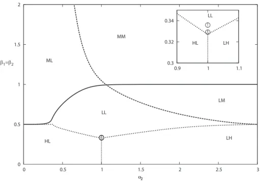
CHAPTER 4. RESULTS ₁₇ 0.3 0.32 0.34 0.9 1 1.1 LL HL LH 0 0.5 1 1.5 2 0 0.5 1 1.5 2 2.5 3 α₂ β₁=β2 MM ML LM LL LH HL

Figure 4.1: Phase diagram of ASEP with two types of particles as function of α2,

for the case α1 = γ1 = γ2 = δ = 1.

extended phase diagram may be labeled by the phases of two decoupled system. The phases are thus labeled as MM, LL, HH, LH, ML, HL, LM. In naming the phases, the first letter stands for the phase of the decoupled ASEP with first type of particles and the second letter stands for the phase of second type of particles.

Fig.4.1 shows the phase diagram when α1 = γ1 = γ2 = δ = 1. Note that the

phases along the α2 = 1 line correspond to the α1 = α2 = 1 line in the phase

diagram found by Evans et al. in Fig. 2.6. As the inset in Fig.4.1 shows the symmetry breaking starts in the LL phase. There is a critical point , which is the endpoint of a line of first order transitions.

In case of densities the order of transitions between phases are also character-ized by the order of phase transitions of one particle ASEP model. Therefore the transition between low density phase and high density phase preserves its first or-der character. When only one of the decoupled systems goes unor-der the transition from L to H or vice versa, the transition is first order but shows no hysteresis. This is the case when there occurs a transition between LL and HL phases or LL and LH phases. If both of the systems undergo the transition from L to H or vice

CHAPTER 4. RESULTS ₁₈

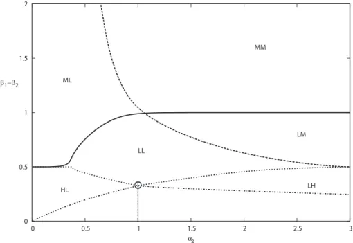
versa, the transition is first order and also shows hysteresis. The reason behind this is the formation of a metastable state due to the initial conditions. To apply MF to a system, it has to be given initial densities. If the initial densities are not consistent with how system has to be due to the α and β values, there occurs a state which is achievable for these initial conditions but not when the parameters are uniformly changed from values for which there is no symmetry breaking. For example HL state, if one chooses the initial conditions which favors higher density for second type of particles, system stays in LH density for a while. When both stable and metastable states exist for certain value of parameters, MF implies infinite life-time. But MC gives finite life-times for transitions between these two states[3]. The line which indicates the where metastability starts when going from β = 0.327 to β = 0 is also added to Fig.4.1. one obtains the diagram in Fig. 4.2. To emphasize the first order transitions, in Fig. 4.3 only the hysteresis

0 0.5 1 1.5 2 0 0.5 1 1.5 2 2.5 3 α₂ β₁=β2 MM ML LM LL LH HL

Figure 4.2: The phase diagram obtained through MF for β = β1 = β2 and

γ1 = γ2 = δ = 1. The line where metastability can be observed is also added to

the Fig. 4.1

curves are drawn for the values β ≤ 0.327.

For α = 1 = α2 = 1 the density symmetric phase ends at about point β = 0.33.

CHAPTER 4. RESULTS ₁₉ 0.2 0.25 0.3 0.35 0.5 1 1.5 2 -1 0 1 ∆ρ β α ∆ρ

Figure 4.3: First order hysteresis curves for density. Hysteresis indicates the double-valuedness of density for small values of β.

at that point. However in between the density symmetric phases and density asymmetric phases there exists a tiny phase. This phase was first observed by Evans et al. For α = 1, β width of this phase is shown in Fig. 4.4 . The phase still exists while α is changing sufficiently away from 1. Taking the logarithm of the β width and corresponding α values one observes linear dependence of these quantities, as can be seen in Fig. 4.5. Mathematically speaking,

log(∆β) ∝ log(α) → ∆β ∝ αA_.

This implies that the change of ∆β with α obeys a power law. Average value of A is found to be 1.17 for right branch, −1.28 for the left branch of the graph.

In case of currents, the characterization of order of phase transition is different. It no more preserves the second order character of current transitions in one type of particle ASEP model. Now it can also be first order. The reason behind this may be the jump in α values itself. As its written before in section 2.2 current value for low density state is given by the formula α(α − 1) and for the high density state it is given by β(β − 1). Therefore no discontinuity in current is expected along the transition line α = β. However, when we solve the simultaneous equation for the two decoupled ASEP system, the solution for

CHAPTER 4. RESULTS ₂₀ -0.8 -0.6 -0.4 -0.2 0 0.2 0.4 0.6 0.8 0.24 0.26 0.28 0.3 0.32 0.34 0.36 0.38 0.4 0.42 β ∆ρ ∆β

Figure 4.4: The tiny phase, where the symmetry starts to be broken but the difference of the values of states are close to each other. ∆β indicates the β width of the phase.

affective values of α itself has a jump along the transition. The graph containing the discontinuities in the current can be seen in Fig.4.6.

In case when δ 6= γ one reaches a system which may no more be characterized by two decoupled ASEP with one type of particles. As can be seen in Fig.4.7 for the values δ is bigger than 1, the current values exceed the maximum value of 0.25. Taking γ = 1 but δ > 1, a particle no more sees empty sites and counter particle sites as indistinguishable. Moreover, it favors the counter particles to the empty sites. This effectively increases the rate at which particles move along the chain.

The tiny phase also exists in this picture for certain values of δ as can be seen in Fig.4.8.

CHAPTER 4. RESULTS ₂₁ 0.0001 0.001 0.01 0.1 1 10 α₂ ∆β

Figure 4.5: ∆β vs α both drawn on logarithmic scale. Here the ∆β is the width in Fig.4.4 0 0.2 0.4 0.6 0.8 1 0 0.5 1 1.5 2 -0.3 -0.25 -0.2 -0.15 -0.1 -0.05 0 0.05 0.1 j1 β α₂ j1

Figure 4.6: 3-D graph of current changes, first order changes are indicated by discontinuities in the lines. Here the currents are also double-valued for small values of β , however it is cut off to show how the current values jump.

CHAPTER 4. RESULTS ₂₂ 0 0.05 0.1 0.15 0.2 0.25 0.3 0.35 0.4 0.45 0.5 0 0.2 0.4 0.6 0.8 1 1.2 1.4 1.6 1.8 2 j1 beta 4 2 1 0.75 0.5

Figure 4.7: The current difference graph for some values of δ. It is seen that for values bigger than δ = 1, current values exceed the maximum value 0.25 .

0.325 0.33 0.335 0.34 0.345 0.35 0.355 0.36 0.365 0.37 0.375 0.5 1 1.5 2 2.5 3 3.5 4 j1 beta

Figure 4.8: Behavior of tiny phase for different values of δ. The tiny phase does not exist for values δ < 0.8

CHAPTER 4. RESULTS ₂₃

4.2

Monte Carlo Simulation

In the Monte Carlo part of the work, computations were done in order to find the density profiles of the system for selected α and β values. Density profiles of the system can be seen in the Fig. 4.9.

0 0.5 1 0 200 1 2 0 0 0.5 1 0 200 1 2 0 0 0.5 1 0 200 1 2 0 0 0.5 1 0 200 1 2 0 0 0.5 1 0 200 1 2 0 0 0.5 1 0 200 1 2 0 0 0.5 1 0 200 1 2 0

Figure 4.9: Some density profiles of the phases as density vs site of the chain. The order of the density profiles from left to right MM, ML, HL, LL for the bottom line HL, LM and LL.

Chapter 5

Conclusion and Future Work

In this thesis, what we did was trying to understand this system via its phase diagram. Mean Field approximation is used to find the phase diagram. Different cross-sections of the system are taken in the six-dimensional space. The idea that

if the hopping rates γ1, γ1 are equal to the exchange rate δ the system ASEP with

two types of particles can be modeled as two decoupled ASEP with one type of

particle systems[3] is generalized to the α1 6= α2 case. Moreover, the new phase

picture of the δ 6= γ is also found. Monte Carlo simulation is used to reach the density profiles of the phases.

As can be seen from the phase diagram of this model; the results are rich in contrast to the simplicity of the model’s dynamics. The model gives a vast oppor-tunity to investigate basic phenomena of the non-equilibrium systems. However, the complexity of the results are challenging to interpret. For a more unified un-derstanding, we will continue on with the Renormalization Group studies which is already in progress.

Bibliography

[1] H. A. Bumstead, R. G. Van Name (eds.), “The scientific papers of J Willard Gibbs (2 volumes)” xi-xxvi (1961).

[2] L. Boltzmann, Wien. Ber. 66 S. 275-370. (1872).

[3] M. R. Evans, D. P. Foster, C. Godr´eche, D. Mukamel, Phys. Rev. E 74, 208 (1995).

[4] B. Derrida, S. A. Janowsky,J. L. Lebowitz, E. R. Speer, J.Stat. Phys. 73, Nos. 5/6 (1993).

[5] T. Antal, G. M. Sch¨utz, Phys. Rev. E 62, 8393 (2000).

[6] Y. Chai, S. Klumpp, M. J. I. Mller, R. Lipowsky, Phys. Rev. E 80, 041928 (2009).

[7] G.M. Sch¨utz, cond-mat/9601082 (1996).

[8] R. A. Blythe, M. R. Evans, J. Phys. A: Math. Theor. 40, R333R441 (2007). [9] B. Derrida, M. R. Evans, V. Hakim, V. Pasquier, J.Phys.A: Math.Gen. 26,

1493 (1993).

[10] I. T. Georgiev, S. R. McKay, Phys. Rev. E, 67, (2003).

[11] T. Hanney, R. B. Stinchcombe, J.Phys.A: Math.Gen. 39, (2006). [12] K.G Wilson, Rev. Mod. Phys. 47, 773-8211;840 (1975).

[13] K. G. Wilson, J. Kogut, Phys. Rep. 12, 75 (1974). 25

BIBLIOGRAPHY ₂₆

[14] M. E. Fisher , Rev. Mod. Phys. 46, 597 8211;616 (1974).

Appendix A

Computer Code

For the calculation of the case δ 6= γ, the following FORTRAN code is used:

double precision prs(7) loop=1000000 prs(1)=1.0 prs(2)=1.0 prs(5)=1. prs(6)=1. prs(7)=1.5 open(3,file="recorddet") do beta=0.33d0 , 0.34d0 , 0.0005d0 prs(3)=beta prs(4)=beta call mean(loop,prs) enddo stop end 27

APPENDIX A. COMPUTER CODE ₂₈

subroutine mean(loop,prs)

implicit double precision (a-h,o-z)

dimension p1(1000),p2(1000),p0(1000),buf1(1000),buf2(1000) dimension prs(7) c write(*,*)"enter a1,a2,b1,b2,g1,g2: " c read(*,*)(prs(i),i=1,6) c prs(7)=1.0 c

c write(*,*)"enter loop no: "

c read(*,*)loop n = 200 dt = 0.1 do i=1,n p1(i)=0.8 p2(i)=0.1 p0(i)=1.0-p1(i)-p2(i) buf1(i)=p1(i) buf2(i)=p2(i) enddo do loopn=1,loop do inner=1,n do i=1,n-1 w10=dt*p1(i)*p0(i+1)*prs(5) w12=dt*p1(i)*p2(i+1)*prs(7) w02=dt*p0(i)*p2(i+1)*prs(6) buf1(i)=buf1(i) -w10-w12 buf1(i+1)=buf1(i+1)+w10+w12

APPENDIX A. COMPUTER CODE ₂₉ buf2(i)=buf2(i) +w02+w12 buf2(i+1)=buf2(i+1)-w02-w12 enddo buf1(1)=buf1(1)+dt*p0(1)*prs(1) buf1(n)=buf1(n)-dt*p1(n)*prs(3) buf2(1)=buf2(1)-dt*p2(1)*prs(4) buf2(n)=buf2(n)+dt*p0(n)*prs(2) dif=0. do i=1,n if(abs(p1(i)-buf1(i)) .gt. dif)dif=abs(p1(i)-buf1(i)) if(abs(p2(i)-buf2(i)) .gt. dif)dif=abs(p2(i)-buf2(i)) p1(i)=buf1(i) p2(i)=buf2(i) p0(i)=1.0-buf1(i)-buf2(i) enddo enddo

c if(mod(loopn,1+loop/20) .eq. 0)write(*,*)loopn," diff=",dif

if(dif .lt. 1e-8)goto 25 enddo 25 ro1=0. ro2=0. do i=1,n ro1=ro1+p1(i) ro2=ro2+p2(i) enddo write(3,*)prs(3),ro1/n,ro2/n,p0(1)*prs(1),p2(1)*prs(4) write(*,*)"final diff=",dif," record: ",prs(3),ro1/n,ro2/n,

APPENDIX A. COMPUTER CODE ₃₀ c open(1,file="probs") c do i=1,n c write(1,*)i,p1(i),p2(i),p1(i)-p2(n+1-i) c enddo return end

APPENDIX A. COMPUTER CODE ₃₁

This following FORTRAN program is used to calculate the extended phase diagram:

open(1,file="record_1.5") alpha1 = 1.0

alpha2 = 1.5

write(1,*)"#R L alpha1 beta1 alpha2 beta2",

1 " J1 J2 d1 d2" do i=200,10,-1 beta1 = 0.01*i beta2 = beta1 call bseps(alpha1,beta1,alpha2,beta2, 1 currp,currm,densp,densm,iphase1,iphase2) write(1,100)iphase1,iphase2,alpha1,beta1,alpha2,beta2, 1 currp,currm,densp,densm 100 format(2i2,8f10.3) enddo stop end subroutine bseps(alpha1,beta1,alpha2,beta2, 1 currp,currm,densp,densm,iphase1,iphase2) densp1= 0.8 denspn= 0.8 densm1= 0.1 densmn= 0.1 alpha1e=alpha1 alpha2e=alpha2

APPENDIX A. COMPUTER CODE ₃₂

do i=1,1000

alpha1e=0.9*alpha1e +

1 0.1*alpha1*(1. - densp1 - densmn)/(1. - densp1)

alpha2e=0.9*alpha2e +

1 0.1*alpha2*(1. - denspn - densm1)/(1. - densm1)

call aseps(alpha1e,beta1,currp,densp,densp1,denspn,iphase1) call aseps(alpha2e,beta2,currm,densm,densm1,densmn,iphase2) if(i .gt. 90 .and. .false.)then

write(1,*)" ae beta curr dens dens1 densn phase"

write(1,200)alpha1e,beta1,currp,densp,densp1,denspn,iphase1 write(1,200)alpha2e,beta2,currm,densm,densm1,densmn,iphase2 200 format(f10.7,5f6.3,i4) endif enddo c stop return end subroutine aseps(alpha,beta,curr,dens,dens1,densn,iphase)

if(alpha .lt. 0.5 .and. beta .gt. alpha)then c LD

iphase=1

curr= alpha*(1. - alpha) dens= alpha

dens1= alpha

densn= alpha*(1. - alpha)/beta return

endif

APPENDIX A. COMPUTER CODE ₃₃

c HD

iphase= 2

curr= beta*(1. - beta) dens= 1.-beta dens1= 1. - beta*(1.-beta)/alpha densn= 1. - beta return endif c MC iphase= 3 curr= 0.25 dens= 0.5 dens1= 0.25/alpha densn= 0.25/beta return end

APPENDIX A. COMPUTER CODE ₃₄

For the Monte Carlo simulation of density profiles the following FORTRAN code is used: dimension lat(1000),rate(1002),n_pos(1002),i_type(1002),params(7) dimension iones(1000),itwos(1000) write(*,*)"enter a1,a2,b1,b2,g1,g2: " read(*,*)(params(i),i=1,6) params(7)=1.0 write(*,*)"enter mcs: " read(*,*)mmcs n=200 m=n+2 num_1=0 num_2=0 do i=1,n iones(i)=0 itwos(i)=0 lat(i)=0 rr=rand() if(rr .lt. 0.25 )then lat(i)=1 num_1=num_1+1 endif if(rr .gt. 0.75 )then lat(i)=2 num_2=num_2+1 c lat(i)=1 c num_1=n c num_2=0 endif

APPENDIX A. COMPUTER CODE ₃₅ enddo call fill(n,m,m_max,r_max,lat,rate,n_pos,i_type,params) t=0. open(2,file="vary") n_stat=0 s_c12=0. ss_c12=0. do mcs=1,mmcs i12=0 c1=0. c12=0. do loop=1,n*n choice=rand()*r_max call select(n,m,m_max,choice,lat,rate,n_pos,i_type, 1 num_1,num_2,jl1,jl2,jr1,jr2) i12=i12+num_1-num_2 c1=c1+jl1*r_max c12=c12+(jl1-jl2)*r_max call fill(n,m,m_max,r_max,lat,rate,n_pos,i_type,params) enddo

c if(i12 .ge. 0)then

n_stat=n_stat+1 do i=1,n

if(lat(i) .eq. 1)then iones(i)=iones(i)+1

APPENDIX A. COMPUTER CODE ₃₆

else if(lat(i) .eq. 2)then itwos(i)=itwos(i)+1 endif

enddo

c endif

c if(i12 .le. 0)then

c n_stat=n_stat+1

c do i=1,n

c if(lat(i) .eq. 1)then

c itwos(n-i+1)=itwos(n-i+1)+1

c else if(lat(i) .eq. 2)then

c iones(n-i+1)=iones(n-i+1)+1

c endif

c enddo

c endif

c n*n samples, density = total/n

d12=float(i12)/(n*n*n)

c one time unit ~ n/r_max; current = count/time

c1=c1/(n*n) c12=c12/(n*n) s_c12 =s_c12+abs(c12) ss_c12=ss_c12+c12*c12 write(2,500)mcs,d12,c1,c12 500 format(i5,1p3e10.2) enddo open(1,file="stats") aa=1.0/n_stat do i=1,n write(1,300)i,iones(i)*aa,itwos(i)*aa, 1 (iones(i)-itwos(n-i+1))*aa 300 format(i4,1p3e9.2)

APPENDIX A. COMPUTER CODE ₃₇ enddo write(*,*)"dj_av: ",s_c12/mcs, 1 " sd: ",sqrt(ss_c12/mcs-(s_c12/mcs)**2) write(1,*)"# dj_av: ",s_c12/mcs, 1 " sd: ",sqrt(ss_c12/mcs-(s_c12/mcs)**2) write(1,400)(lat(i),i=1,n) 400 format("# ",100i1) stop end subroutine fill(n,m,m_max,r_max,lat,rate,n_pos,i_type,params) dimension lat(n),rate(m),n_pos(m),i_type(m),params(7) m_max=0 r_max=0.

if(lat(1) .eq. 0)then

call push(m,1,1,m_max,r_max,rate,n_pos,i_type,params) else if(lat(1) .eq. 2)then

call push(m,1,4,m_max,r_max,rate,n_pos,i_type,params) endif

if(lat(n) .eq. 0)then

call push(m,n,2,m_max,r_max,rate,n_pos,i_type,params) else if(lat(n) .eq. 1)then

call push(m,n,3,m_max,r_max,rate,n_pos,i_type,params) endif

do i=1,n-1 ii=i

APPENDIX A. COMPUTER CODE ₃₈

if(lat(i) .eq. 0 .and. lat(i+1) .eq. 2)then

call push(m,ii,6,m_max,r_max,rate,n_pos,i_type,params) else if(lat(i) .eq. 1 .and. lat(i+1) .eq. 2)then

call push(m,ii,7,m_max,r_max,rate,n_pos,i_type,params) else if(lat(i) .eq. 1 .and. lat(i+1) .eq. 0)then

call push(m,ii,5,m_max,r_max,rate,n_pos,i_type,params) endif enddo return end subroutine push(m,i,k,m_max,r_max,rate,n_pos,i_type,params) dimension rate(m),n_pos(m),i_type(m),params(7) m_max=m_max+1 r_max=r_max+params(k) rate(m_max)=r_max n_pos(m_max)=i i_type(m_max)=k c write(*,200)m_max,r_max,i,k 200 format(i3,f5.1,2i3) return end subroutine select(n,m,m_max,choice,lat,rate,n_pos,i_type, 1 num_1,num_2,jl1,jl2,jr1,jr2) dimension lat(n),rate(m),n_pos(m),i_type(m) jl1=0 jl2=0 jr1=0 jr2=0

APPENDIX A. COMPUTER CODE ₃₉

do i=1,m_max

if(rate(i) .ge. choice) exit enddo k=n_pos(i) if(i_type(i) .gt. 4)then itemp=lat(k) lat(k)=lat(k+1) lat(k+1)=itemp

else if(i_type(i) .eq. 1)then lat(1)=1

num_1=num_1+1 jl1=1

else if(i_type(i) .eq. 2)then lat(n)=2

num_2=num_2+1 jr2=1

else if(i_type(i) .eq. 3)then lat(n)=0

num_1=num_1-1 jr1=1

else if(i_type(i) .eq. 4)then lat(1)=0 num_2=num_2-1 jl2=1 endif c write(*,*)(" ",ii=1,14+k),"-" c write(*,100)choice,i,k,i_type(i),(lat(ii),ii=1,n) 100 format(f5.2,2i4,i2," ",100i1) return end