REGENERATOR PLACEMENT IN OPTICAL
NETWORKS
a thesis
submitted to the department of industrial engineering
and the institute of engineering and science
of bilkent university
in partial fulfillment of the requirements
for the degree of
master of science
By
Onur ¨
Ozk¨ok
January, 2004
I certify that I have read this thesis and that in my opinion it is fully adequate, in scope and in quality, as a thesis for the degree of Master of Science.
Assist. Prof. Dr. Oya Ekin Kara¸san (Supervisor)
I certify that I have read this thesis and that in my opinion it is fully adequate, in scope and in quality, as a thesis for the degree of Master of Science.
Assoc. Prof. Dr. Osman Oˇguz
I certify that I have read this thesis and that in my opinion it is fully adequate, in scope and in quality, as a thesis for the degree of Master of Science.
Assist. Prof. Dr. Bahar Yeti¸s Kara
Approved for the Institute of Engineering and Science:
Prof. Dr. Mehmet B. Baray
Director of the Institute Engineering and Science ii
ABSTRACT
REGENERATOR PLACEMENT IN OPTICAL
NETWORKS
Onur ¨Ozk¨ok
M.S. in Industrial Engineering
Supervisor: Assist. Prof. Dr. Oya Ekin Kara¸san January, 2004
Increase in the number of users and resources consumed by modern applications results in an explosive growth in the traffic on the Internet. Optical networks with higher bandwidths offer faster and more reliable transmission of data and allows transmission of more data. Fiber optical cables have these advantages over the traditional copper wires. So it is expected that optical networks will have a wide application area.
However, there are some physical impairments and optical layer constraints in optical networks. One of these is signal degradation which limits the range of optical signals. Signals are degraded during transmission and below a threshold the signals become useless. In order to prevent this, regenerators which are capable of re-amplifying optical signals are used. Since regeneration is a costly process, it is important to decrease the number of regenerators used in an optical network.
To increase the reliability of the network, two edge-disjoint paths between each terminal on the network are to be constructed. So the second path could be used in case of a failure in transmitting data on an edge of the first path. Considering these requirements, selecting the nodes on which regenerators are to be placed is an important decision.
In this thesis, we discuss the problem of placing signal regenerators on optical networks with restoration. An integer linear program is formulated for this prob-lem. Due to the huge size and other problems of the formulation, it is impractical to use it on large networks. For this reason, a fast heuristic algorithm is proposed to solve this problem. Three methods are proposed to check the feasibility when a fixed set of regenerators are placed on specific nodes. Additionally, a branch and bound algorithm which employs the proposed heuristic is developed to find
iv
the optimal solution of our problem. Performance of both the heuristics and the branch and bound method are evaluated in terms of number of regenerators placed and solution times of the algorithms.
Keywords: optical networks, regenerator placement, branch and bound algorithm,
¨
OZET
OPT˙IK A ˘
GLARDA REJENERAT ¨
OR
KONUMLANDIRILMASI
Onur ¨Ozk¨ok
End¨ustri M¨uhendisli˘gi, Y¨uksek Lisans Tez Y¨oneticisi: Yard. Do¸c. Dr. Oya Ekin Kara¸san
Ocak, 2004
Kullanıcı sayısındaki ve modern uygulamaların kullandı˘gı kaynaklardaki artı¸s, internet ¨uzerindeki trafikte hızlı bir b¨uy¨umeye yol a¸cmı¸stır. Optik a˘glar, daha ¸cok veriyi, daha hızlı ve daha g¨uvenli ¸sekilde iletme imkanı sunmaktadır. Fiber optik kabloların, geleneksel bakır tellere g¨ore bu avantajları vardır. Bu nedenle optik a˘gların geni¸s bir uygulama alanı bulması beklenmektedir.
Ancak, optik a˘glarda bazı fiziksel uyumsuzluklar ve optik katman kısıtları vardır. Bunlardan biri, optik sinyallerin menzilini kısıtlayan sinyal zayıflamasıdır. Sinyaller iletim sırasında zayıflamakta ve belli bir e¸sik de˘gerinin altında kullanılmaz hale gelmektedir. Bunu ¨onlemek i¸cin optik sinyalleri yeniden g¨u¸clendirebilen rejenerat¨orler kullanılmaktadır. Sinyal rejenerasyonu maliyetli bir i¸slem oldu˘gundan, optik a˘glarda kullanılan rejenerat¨or sayısını azaltmak ¨onemlidir.
A˘gın g¨uvenilirli˘gini artırmak i¸cin, a˘g uzerindeki her d¨u˘g¨um ¸cifti arasında iki ayrık yol bulunmalıdır. B¨oylece, ¸calı¸san yol ¨uzerindeki bir ayrıt veri iletiminde ba¸sarısız olursa, onarım yolu kullanılarak veri hedefine iletilebilinir. B¨ut¨un bu gereklilikleri g¨oz ¨on¨une alarak hangi d¨u˘g¨umlere rejenerat¨or yerle¸stirelece˘gini be-lirlemek ¨onemli bir karardır.
Bu tez ¸cal¸smasında, onarımlı optik a˘glarda sinyal rejenerat¨orleri konum-landırılması problemi ¨uzerinde ¸calı¸smaktayız. Bu problem i¸cin bir tamsayılı do˘grusal karar modeli geli¸stirilmi¸stir. Ancak modelin boyutunun ¸cok b¨uy¨uk ol-ması ve modeldeki ba¸ska sorunlar nedeniyle, modelin b¨uy¨uk a˘glarda kullanılol-ması pratik de˘gildir. Bu nedenle, problemin ¸c¨oz¨um¨u i¸cin hızlı ¸calı¸san sezgisel bir al-goritma ¨onerilmi¸stir. Belirli d¨u˘g¨umlere rejenerat¨or yerle¸stirilmesini i¸ceren bir ¸c¨oz¨um k¨umesinin olurlu˘gunu kontrol eden ¨u¸c farklı y¨ontem ¨onerilmi¸stir. ˙Ilaveten,
vi
¨onerilen sezgisel algoritmayı da kullanarak eniyi ¸c¨oz¨um¨u bulan bir dsınır al-goritması geli¸stirilmi¸stir. Hem sezgisel algoritmaların, hem de dal-sınır algorit-masının performansları, konumlandırılan rejenerat¨or sayısı ve ¸c¨oz¨um zamanları a¸cısından de˘gerlendirilmi¸stir.
Anahtar s¨ozc¨ukler : optik a˘glar, rejenerat¨or konumlandırılması, dal-sınır
Acknowledgement
First and foremost, I wish to express my thanks to Dr. Oya Ekin Kara¸san for introducing me to this interesting and challenging subject and her guidance throughout the development of this thesis. I would also like to thank her for her considerable encouragement and tolerance during my graduate study. Without her support it would not have been possible for me to complete my graduate study. I would also like to thank Dr. Osman O˘guz and Dr. Bahar Yeti¸s Kara for their comments and helpful suggestions for the preparation of this text.
I would like to express my gratitude to Dr. ˙Imdat Kara for his support and encouragement during my graduate study. I am grateful to my roommates Demiralp Hatipo˘glu for helping me to draw the figures and Tolga Bekta¸s for his comments. Thanks to Onur Ak¨oz, Erg¨un Eraslan, Yazgı T¨ut¨unc¨u and Bu˘gra C¸ amlıca for their patience, understanding and encouraging support.
I would also like to express my deepest gratitude to my family and my friend Sezen Altınova and appreciate their endless support throughout my education and life.
Contents
1 Introduction 1
1.1 Problem Definition . . . 7
1.2 Organization of the Thesis . . . 9
2 Related Work 10 2.1 Network Reliability and Regenerator Placement . . . 10
2.2 Regenerator Placement . . . 11
2.3 Network Reliability . . . 13
3 Difficulties in Modelling the Problem 16 3.1 Integer Linear Program For the Entire Graph . . . 17
3.2 Integer Linear Program For a Specific Pair . . . 20
3.3 Problem With the Integer Linear Program . . . 21
3.4 Solution Approach to the Problem in Model2 . . . 24
3.4.1 Modified Integer Linear Program . . . 25
3.5 Mathematical Program in Practice . . . 34 viii
CONTENTS ix 4 Feasibility of an Instance 37 4.1 Using Model2 . . . 37 4.2 Exact Feasibility . . . 38 4.3 Approximate Feasibility . . . 44 5 Heuristic Solutions 47 5.1 Proposed Heuristic Algorithm . . . 47
5.2 Computational Analysis . . . 50
6 Finding an Optimal Solution 52 6.1 Lower Bound of the Problem . . . 52
6.2 Branch and Bound Algorithm . . . 53
6.2.1 Adaptation of the Branch and Bound Algorithm . . . 54
6.3 Computational Analysis . . . 58
List of Figures
1.1 Transparent and Translucent Lightpaths . . . 4
1.2 Restoration Methods . . . 6
3.1 14-node network . . . 20
3.2 A small example . . . 22
3.3 a)Original Graph b)Modified Graph (EC=2) . . . 25
3.4 Rings in a path . . . 27
3.5 Visiting a vertex more than twice . . . 33
3.6 Network topology used in experiments . . . 35
4.1 Path matchings . . . 45
6.1 Branch and Bound Tree . . . 55
6.2 Branch and Bound Tree- Eliminated . . . 56
List of Tables
3.1 Path lengths. . . 23
3.2 Modified Graph with EC=2. . . 24
3.3 Rings in a path. . . 29
3.4 Some of the paths which represent P1 . . . 30
3.5 Optimality Ranges. . . 32
3.6 Multi visited vertices. . . 33
4.1 Running Times For Feasibility Check. . . 38
4.2 Path Alternatives. . . 42
4.3 Number of Path Alternatives. . . 43
5.1 Heuristic Solutions for 32 node network. . . 50
5.2 Heuristic Solutions for 50 node network. . . 50
6.1 Optimal and Heuristic Solutions for the 32 node network. . . 59
6.2 Optimal and Heuristic Solutions for the 50 node network. . . 59
To My Family. . .
Chapter 1
Introduction
Since the initial deployment of the original ARPANET which was developed by Advanced Research Projects Agency (ARPA) and became the basis for the Inter-net, Internet architecture has evolved in response to technological progress and user needs. The explosive growth in traffic fed by the increase in the number of users and resources consumed by modern applications has put an ever increas-ing load on the Internet. A report from the U.S Department of Commerce [3] suggests that the rate at which the Internet has been adopted has surpassed all other technologies preceding it, including radio, television, and the personal computer. A common expectation is the convergence of voice, video, and data communications to happen over the Internet. With this rising of the Internet there have arisen corresponding requirements for network reliability, efficiency, and Quality of Service (QoS) [4]. There are different definitions about QoS. In a general context, QoS is a set of methods and processes which a service based or-ganization implements to maintain a specific level of quality. It is also the ability for an application to obtain the network service it requires for successful oper-ation. To respond to this challenge, Internet service providers (ISPs) examine their operational environment to scale their networks and optimize performance. ISPs employ three complementary technical instruments:
Network architecture It is the abstract structure of the network. It involves 1
CHAPTER 1. INTRODUCTION 2
the components or object classes of the network, their functions and the relations between them.
Capacity expansion This is employed as a response to the traffic growth by the large ISPs.
Traffic engineering This is used to address the Internet growth, and has at-tracted significant attention at recent times.
Development of Optical Transport Networks is seen as an important step in the evolution of data transmission. Fiber optic cables are used in the optical networks and the paths through which data are transmitted are referred to as lightpaths. These optical networks have emerged as an alternative to traditional copper wire or wireless networks, because they can transfer more data at higher speeds than copper wire. Optical networks could handle the increasing traffic on the Internet since multiple signals can be sent simultaneously. Copper wires, on the other hand, can send only one signal at a much slower speed. It is expected that the amount of information carried on computer and telecommunication networks will grow very rapidly in the future, therefore optical networks are likely to play an important role.
However, optical networks have some disadvantages, in addition to their ben-eficial properties. Some transmission impairments make some signal routes unus-able in optical networks. These impairments are discussed in [13]. One of these impairments is the degradation of the signal. An optical signal has a
signal-to-noise (SNR) ratio, which may be considered as the quality of the signal. In
optical networks, signals are degraded during emission from a node [13]. Below a threshold value, the signal cannot be used. So an acceptable SNR level, which depends on the properties of the optical network, needs to be maintained at the receiver [13].
The amount of the degradation depends on the length of the fiber optic cable. For this reason, with current technology at hand, the physical layer constraints limit the maximum transmission range for optical signals. Beyond this length, the optical signals are degraded, and the SNR becomes too low to be usable.
CHAPTER 1. INTRODUCTION 3
In such cases the optical signal must be regenerated to increase the transmission range of the optical network. This regeneration process is called 3R Regeneration, which refers to re-amplification, re-shaping and re-timing of optical signals [23].
Since it is possible to transmit data along the fibers, optical networks are represented using undirected graphs. The vertices (nodes) of the graph represent the receivers and the edges of the graph are used to represent the fiber connections of the network.
The nodes on optical networks are called optical cross connects (OXC). There are two types of optical nodes in an optical network. The first one is transparent node and the second is opaque node. Transparent nodes receive and send the optical signal to another node, whereas the opaque nodes receive, regenerate and send the optical signal to its destination. How the opaque nodes regenerate the optical signals is beyond the scope of this work and will not be discussed.
Optical networks can be classified into three main classes according to the regeneration functions of their nodes [18].
Transparent A network is referred to as transparent if its nodes are optical cross connects without any regeneration function.
Opaque When regeneration is available at every node, the network is called an opaque network.
Translucent If regeneration is available on some nodes of the network, then it is called a translucent network.
Each type of network has its advantages and disadvantages. We will briefly men-tion them. In a transparent network, it is required that lightpaths can reach any destination with required signal-to-noise ratios (SNRs) because payload regener-ation is not available en route. Consequently, in such a network there is a critical diameter above which it cannot extend with given optical transmission technol-ogy. Opaque networks do not have this drawback, on the other hand cost, space, power and reliability implications prevent using these networks widely [18].
CHAPTER 1. INTRODUCTION 4
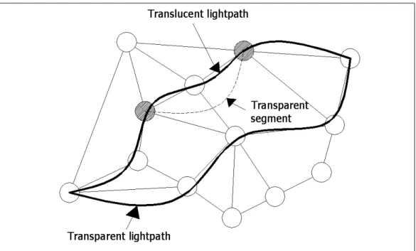
Figure 1.1: Transparent and Translucent Lightpaths
Translucent networks lie between these two extreme cases. To establish a connection under optical impairments, it is necessary to divide some lightpaths into two or more fragments using regenerators [15]. Therefore in a translucent network, there are two types of lightpaths. A lightpath is called translucent
lightpath if there are some opaque nodes en route, otherwise it is called transparent lightpath. Note that the path segments between two opaque nodes are transparent
lightpaths [18, 23]. Transparent and translucent lightpaths can be seen in Figure (1.1).
There is strong interest in implementing transparent all-optical networks due to significant cost saving in not regenerating optical signals in transit nodes. Unfortunately, those impairments mentioned above limit the transparent length of a transparent lightpath. At present and in the foreseeable future, regeneration is necessary to establish a lengthy end-to-end lightpath [23].
Using networks of transparent islands is another way of getting benefits of both transparent and opaque networks. In such networks, the optical network is divided into islands (domains) each of which is a transparent network itself.
CHAPTER 1. INTRODUCTION 5
Regenerators are placed on the boundaries of the islands. In an island, signals reach destinations without regeneration. However, for communication between different islands, signals are regenerated on the boundaries [18].
It is known that translucent networks are superior to opaque networks in the sense of cost structure. Performance, however, is another important aspect. Experiments showed that about 20% of regeneration nodes are needed to achieve a performance close to an opaque network [22]. Therefore, translucent networks could be used instead of opaque networks without a decrease in the performance of the network. However, placing the regenerators on the network such that we achieve the performance of an opaque network using the minimum number of regenerators is a challenging problem [15]. Although the necessity of signal regeneration is discussed, efficient regenerator placement problem is not dealt with widely.
Connectivity is the major concern of the network routing protocols deployed today. An important component of Quality of Service (QoS) is the ability of the network to transport data reliably and efficiently.
Connections of the network may be subject to failure [1]. In case of a failure, we need to respond to this failure and transport the data somehow to its desti-nation. For this reason, some techniques are needed to recover the failure and these techniques are called Recovery Methods. When a lightpath is broken due to a failed connection of the network, another lightpath must be established in order to transport the signal to its destination. Recovering the failure in fact is constructing this new lightpath, rather than to repair the failed connection.
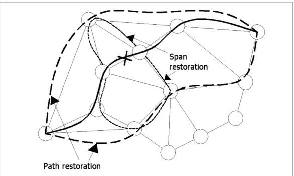
Recovery methods can be classified based on the scope of the recovery action. Some methods are explained in [18, 24]. Local Repair, also known as Span-based
Restoration, aims to protect against single link or node failures. In this case,
failure detection and restoration are carried out between the two terminating nodes of the failed connection. So, the recovery path shares overlapping portions with the working path. Global Repair which is also known as Path Restoration or Path-based Restoration aims to protect against any link or node failure on the working path. In many cases the restoration path may be selected to be link
CHAPTER 1. INTRODUCTION 6
Figure 1.2: Restoration Methods
or node disjoint from the working path to protect against all link and/or node failures on the working path [18, 24]. In a span-restorable network, the failure detection and restoration are carried out between the two terminating nodes of a failed span [18]. Since the response is local, span-restoration is thought of as being fast but with relatively lower space capacity efficiency. In contrast, a path-restorable network is more efficient in spare capacity but often has a slower restoration speed [18]. Examples of span-based and path-based restoration can be seen in Figure (1.2).
The networks, in which path-based restoration is preferred, should be de-signed such that there is a restoration-path disjoint from the working-path in the network. Diversity is a relationship between ligthpaths. Two lightpaths are said to be diverse if they have no single point of failure. Diversity is often equated to routing two lightpaths between a single pair of points, or different pair of points, so that no single failure will disrupt them both [13].
For this reason, the networks must be designed such that in case of a failure the network should still remain active. This problem is called survivable network
CHAPTER 1. INTRODUCTION 7
design problem (SDNP). This problem has applications to the design of survivable
telecommunication networks [10]. With the introduction of optic technology in telecommunication, designing a minimum cost survivable network has become a major objective in the telecommunication industry [12]. In optical networks, 2-edge connected networks in which there are at least two edge disjoint paths between each pair of terminals have shown to be cost effective and provide an adequate level of survivability [10]. The 2-edge connected subgraph problem, a special case of SDNP, is known to be NP-hard [14].
Next step in network survivability is the Two edge-disjoint Hop-constrained
Paths Problem (THPP). Regarding the reliability of a telecommunication
net-work, having two edge-disjoint paths is often insufficient [12]. The alternative path (restoration path) could be too long to guarantee an effective routing, which may result in degradation of the signal. In such cases, L-path requirement guar-antees exactly the needed quality for the paths [12]. L-path requirement means that there can be at most L nodes in a path.
In this thesis, an optical network which is assumed to transmit data between two terminal nodes will be designed. In the design problem, a given transparent network will be transformed into a survivable translucent network to gain the range of an opaque network with minimum cost. Since the cost of regenerator nodes is the dominant factor, deciding on where to place regenerator nodes is an important problem. In this thesis, an effective method is proposed for placing the regenerator nodes and routing the signals through two-edge disjoint paths.
1.1
Problem Definition
Having defined optical networks and their physical impairments, we want to state the problem for which we will propose solution methods in this study.
Let G(V, E) be an undirected graph with n vertices (nodes) and m edges, and
c(E) be the vector representing the lengths of the edges in G. Assume that this
CHAPTER 1. INTRODUCTION 8
attenuation the signal degrades through the edge. Our aim is to send a signal from each vertex to all other vertices within the prespecified degradation limit.
Assume that, path-based restoration as explained before in this chapter, is to be incorporated in this optical network. Therefore, we need to find alternative ways to send the signal. The more number of disjoint paths we have, the more reliable the network is. Nevertheless, as the number of disjoint paths increases, it becomes harder to find these paths. Finding the number of disjoint paths to make the network reliable enough is beyond the scope of this work. Generally, two disjoints paths are assumed to be sufficient in the literature [10] and we adopt this assumption. By this way, the reliability of the network is increased. Therefore, we are going to find two edge-disjoint paths between all pairs of vertices of G.
The second point is the degradation limit. As explained before, a signal attenuates in time after it is sent from a vertex and after a period it will be completely lost. This amount of degradation (threshold value) after which the signal becomes useless is called the degradation limit. Therefore the signal must arrive at its destination within the degradation limit otherwise it would be lost. This means, the lengths of the paths we find through which the signal is sent must be within the degradation limit. There is no problem if we can find paths that have reasonable lengths. What can be done if there are not such paths? In such cases, a device called regenerator could be used to regenerate the signals. Regenerators are devices that receive and resend the signal in order to realize the regeneration process mentioned in this chapter. By this way, the signal will be recovered and will not be lost until degradation limit is reached. Think of a path that passes through a vertex on which there is a regenerator. We can divide this path into two, from the vertex with regenerator. First part starts from the source vertex and ends at the regenerator vertex, and the second part starts from regenerator vertex and ends at the terminal vertex. Each part of the path between neighboring opaque nodes will be referred to as sub-paths. Remember that these sub-paths are the same with the transparent path-segments described previously in this chapter. Having defined what a sub-path is, it can easily be seen that a path could have more sub-paths than two. The number of sub-paths depends on the number of regenerators that the path passes through. If there is one
CHAPTER 1. INTRODUCTION 9
regenerator, then there are two sub-paths. With four regenerators, for example, there will be five sub-paths. Using regenerators, we can relax the degradation limit constraint. Now, it is not necessary for the paths as wholes to be within the degradation limit, it is sufficient if each sub-path is within the degradation limit. It is assumed that there are two edge-disjoint paths between all pairs of the graph. This means that using sufficient number of regenerators, paths that satisfy degradation constraint could be constructed. The regenerator, however, is an expensive device so we want to minimize the total number of regenerators placed on the network. Therefore, our problem is to determine the minimum number of regenerators that would be sufficient to satisfy the degradation constraint and to decide where the regenerators should be placed.
1.2
Organization of the Thesis
In this thesis, we formulate the regenerator placement problem as an integer linear program. Since the solution of this problem, due to its size, is very hard, we develop and implement a heuristic approach. After this, we propose a branch and bound algorithm which employs the heuristic, to find the optimal solution. We obtain numerical results for these approaches on sample networks and compare their results and efficiencies with those of the solution methods which have been proposed in [24, 25].
The thesis is organized as follows: Chapter 2 summarizes the studies in the literature on network reliability and regenerator placement and on finding edge-disjoint paths. In Chapter 3, an integer linear formulation of this problem, the difficulties in modelling and solving the problem are discussed. Chapter 4 includes the methods to check the feasibility of a fixed set of regenerators placed at specific vertices and explains why even the feasibility check is a difficult problem. In Chapter 5, a heuristic algorithm is proposed and numerical results are obtained. Another method which finds the optimal solution of the problem is developed in Chapter 6. Numerical results are also provided in this chapter. Finally, Chapter 7 concludes the thesis.
Chapter 2
Related Work
As stated in Section (1.1) our problem has two main aspects. The first one is network reliability and the second one is respecting the degradation limit i.e. regenerator placement. Both subjects have been studied and research about them could be found in the literature. In this chapter, we will give the research about these subjects. These two subjects seem to be independent but in fact they are inter-related. Therefore we want to discuss the literature in which both problems are studied together first, and then we will look at the studies in which these subjects are examined individually.
2.1
Network Reliability and Regenerator
Place-ment
Our problem consists of two main components, the first one is network reliability and the second one is deciding on the places of regenerators. In our problem, survivable networks are designed according to path-restoration technique, hence two edge-disjoint paths are to be found between each pair (s, t) ∈ V of the graph. Related work about this subject is given in Section (2.3). The work done about the second part of the problem, regenerator placement, is given in Section (2.2).
CHAPTER 2. RELATED WORK 11
In these works, only one part of our problem is studied separately, however, both parts are closely related in our analysis. Works that take both components into account are given in this section. Unfortunately this subject has not been widely studied. We have found only two published work on this problem.
Capacities of the fiber links are also important since data cannot be trans-mitted if the capacity of a link is exceeded. For this reason, the traffic flow on the network should be controlled to prevent exceeding the capacities in data transmission. This control process is called traffic engineering.
Yetginer, who mainly focused on traffic engineering, partially studied regen-erator placement in [24]. In a closely related article [25], the same subject is investigated. In both studies, traffic engineering is the main focus. They have introduced a nonlinear integer program to solve the problem. However, due to its size, they could not solve the program. Two heuristic algorithms are proposed but they have not discussed the efficiency of their solutions. Besides, their non-linear integer program may fail to find the optimal solution even if its size were reasonable. To overcome this, authors in [24, 25] bring in an additional assump-tion to restrict the soluassump-tion space. This will be fully discussed in Chapter 3. Our analysis, however, will relax this assumption.
2.2
Regenerator Placement
In [18], there is a different approach to optical signal recovery, where regener-ators (opaque nodes) are used to detect failures. Two basic restoration tech-niques, path-based and span-based restoration, were described in Chapter (1). The approach in [18] is an intermediate and more general option, called segment-based survivability. Segment-segment-based survivability schemes carry out restoration of a failed path segment between the opaque nodes upstream and downstream of the actual span failure. Remember, this segment is the transparent fragment (sub-path) in other words signals are not regenerated except from the source and terminating nodes of the sub-path. Based on segment-based survivability,
CHAPTER 2. RELATED WORK 12
opaque node (regenerator) placement problem is solved using a heuristic algo-rithm in [18]. A method to find the optimal solution and alternative optima is described and implemented. However the optimal solution technique is nothing but complete enumeration. There is not any intelligent search technique em-ployed to traverse the solution space. Therefore this method is not efficient. The optimal and heuristic solutions are compared. Although the heuristic solutions are worse than the optimal solution, the running times of the heuristic are very effective.
Routing and wavelength assignments are considered jointly in [23]. Although, this study considers the need for regeneration, it uses a different approach. In-stead of adding regenerator nodes to the network, some nodes that have spare capacity, are used as regenerators. We are not interested in the mechanism of using ordinary nodes as regenerator nodes. The nodes which will be used as re-generators are determined using two different algorithms. These algorithms take the blocking probability of the signal due to wavelength unavailability into ac-count. After deciding on the places of the regenerator nodes, routing algorithms are employed. Survivability of the network is not considered in this study [23].
Kim and Seo [15] studied regenerator problem which is similar to the problem in [23]. They did not consider network survivability, but included another factor which is the blocking of the lightpaths throughout the network. They used two approaches to the problem, the first one being a minimal-cost placement which minimizes the blocking of lightpaths using dynamic programming, the second be-ing a heuristic for locatbe-ing the signal regeneration nodes. A comparison between these two algorithms and other ones proposed in different studies is also given in [15].
In the research done by Yang and Ramamurthy [22], regenerator placement problem is examined. In this study, regenerator placement problem is solved offline, i.e. at the design phase of the network. Routing algorithms are used after regenerator places are determined and fixed. They have solved the problem using two heuristic methods and measured the performance of the system with simulation models. Again survivability of the network is not considered.
CHAPTER 2. RELATED WORK 13
2.3
Network Reliability
Network reliability is an important concept in network design problems especially
in communication networks. The problem of network reliability arises from the fact that the edges may be subject to failure [1]. A signal is sent from a vertex to another via some set of edges and vertices. A network reliability problem is to compute the probability that the specified node pair can communicate at a given time i.e. no arc on the path fails to transmit data. Given the probabilities of the edges, the aim is to design more reliable networks. Most network reliability problems are NP-hard [1]. A survey of this problem can be found in [1]. Since we are not interested in probability of communication, we will not go into details here.
The concept of network reliability or network survivability is a bit different in our problem. No matter how reliable a path between a node pair is, the path may fail to transport data from source to the terminal. If a failure occurs, there is a need for a responding strategy about transporting the data from the source to its destination. The responding strategies have been mentioned in Chapter (1). In our problem, path restoration strategy is preferred. Therefore, we need to establish a restoration path in the designing phase of the network. That is to say two paths are to be constructed between a node pair, one as the working path and the other as the restoration path. These two paths can share some edges or can be either edge-disjoint or vertex-disjoint. In our problem edge-disjoint paths are preferred. For this reason, two edge-disjoint paths, lengths of which should be within degradation limit, must be constructed.
Network reliability and survivability are improved if disjoint paths are used between source and terminal nodes in the network [9]. Assuming that the edges and nodes of a network have known reliability, the reliability of a path between two nodes can be computed. The number of edges in a path and the number of disjoint paths are given as an input. In [9], an algorithm is proposed to identify the set of K-most reliable paths. This algorithm calculates the reliability of the paths and outputs them in the decreasing order.
CHAPTER 2. RELATED WORK 14
Survivable network design problem (SNDP) is an important and widely studied
problem. In SNDP problems, a sub-graph of the main graph is formed such that there are two disjoint paths between each pair of the graph. Usually the aim is to minimize the total cost of the subgraph and this resulting problem is NP-hard [11]. Given a graph which is 2-edge connected, a spanning subgraph with minimum number of edges is found. Huh proposed an algorithm is to find the subgraph in [11]. Huygens et al. [12] has also studied such a problem. They try to find a subgraph where the number of the edges in the disjoint paths are constrained. An integer program is formulated and facets of the problem polyhedron are defined. Different versions of this problem in which length of the paths are also constrained could be found in the literature. Kerivin and Mahjoub [14] are also interested in the polyhedron of a special SNDP. Partition inequalities are used in this study and they showed that this problem can be solved in polynomial time in special type of graphs.
Without degradation limit, the problem of finding edge-disjoint paths is widely studied. There are two major kinds of disjoint paths in the literature. In the first type, disjoint paths are found between different pairs of nodes. Such a problem arises in the telecommunication area. Connections interfere with each other if the paths share some edges. The question of how many connections can be made simultaneously could be answered by solving this problem. Most of these problems are NP-complete and an example could be found in [16]. This problem, however is not closely related with our problem.
The second type of problem is to find disjoint paths between a single pair of nodes. Different studies on this problem could be found. Vygen discussed some edge-disjoint problems in his work and showed that they are NP-complete [21]. Brandes et al. developed a software package which includes algorithms for different disjoint problems in planar graphs in [6]. Coupry studied a maximum cardinality set of edge-disjoint paths problem. In this problem, the graph is non-weighted and the aim is to find maximum flow between two nodes where each edge has unit capacity. He proposed a linear algorithm for this problem in [8]. Conforti, Hassin and Ravi used a different approach to this problem. They studied the problem of constructing edge-disjoint paths using previously found
CHAPTER 2. RELATED WORK 15
edge-disjoint paths. Assume that, we look for edge-disjoint paths for the pair (s, t) and say we already know edge-disjoint paths between pairs (s, r) and (r, t). These known paths are combined to solve the problem which is equivalent to the stable matching problem [7].
The problems mentioned above often do not have objective functions. When an objective function, such as minimizing the cost or weighted cost of disjoint paths etc., is inserted to the problem, it gets even harder. It is shown in [17] that the problem of finding two edge-disjoint paths and minimizing the length of the longer one is strongly NP-complete. The underlying network of this problem can be directed or undirected. This problem is of great interest to us, since it is closely related to our problem. Remember the impairments we have discussed in Chapter 1. We have overcome the impairments using regenerator nodes in networks. Assume that we do not want to use regenerator nodes and want to know which pairs can communicate without regeneration. Since two paths are to be established, one working and one restoration path, we should solve the problem stated above. If the length of the longer path is within the degradation limit given, then we can conclude that the pair can communicate without regenerators.
A similar problem to this one, is to find a pair of disjoint paths, shortest pair, so as to minimize the total length of the two paths. Solution techniques to this problem could be found in the literature. For example, Suurballe proposed an algorithm to solve both node disjoint and edge-disjoint versions of the problem [19]. Suurballe and Tarjan improved the algorithm in [19]. They again tried to minimize the total length of the paths, but this time they found the paths between a single source and each possible sink nodes [20]. Banerjee et al. [5] has proposed a parallel algorithm for the two problems, which are single sink and multi sink versions. They used Dijsktra’s shortest path algorithm [2] iteratively to find the shortest pair of disjoint paths. In all problems, the underlying graphs are directed.
Chapter 3
Difficulties in Modelling the
Problem
Our problem, as defined in Section (1.1) is to establish two edge-disjoint paths, one working path and one restoration path, between each pair of vertices of the graph such that the lengths of the paths have to be within the given degradation limit. Remember that our optical network is represented by the undirected graph,
G(V, E). If paths with such lengths cannot be found, regenerators will be placed
on some nodes of the graph. In this case, the paths will be divided into fragments and length of each fragment must be within the pre-specified degradation limit. Here we want to define the length of a path. Although length of a path is a well known term, it is a bit different here, since we are interested in not only the entire path but also the path fragments. Say L(P ) denotes the length of path P and li
denotes the length of path fragment i. Then the length of path P , in which there are k path segments will be, L(P ) = max{l1, l2, . . . lk}
In order to find the optimal solution of our problem, we have attempted to formulate an integer linear program to solve it. Hereafter, this integer linear program will be denoted by Model1. Model1 in its simplest form may fail to find the optimal solution. We have developed a technique to overcome this problem. In this chapter we will introduce Model1, discuss its drawbacks and show how
CHAPTER 3. DIFFICULTIES IN MODELLING THE PROBLEM 17
to use it iteratively to find the optimal solution. Although G is an undirected graph, directions are important in signal transportation. For this reason, we transform G(V, E) into a directed network G(N, A). To do this, each undirectedb
edge {i, j} ∈ E is replaced by two directed arcs (i, j) and (j, i), both with cost c({i, j}) [2]. Therefore, the directed networkG which will be used in formulatingb
Model1 and other integer linear programs (ILPs) has n nodes and 2m directed arcs.
3.1
Integer Linear Program For the Entire
Graph
To find the optimal solution to this problem a mathematical program is formu-lated. This model shows some similarities with the one introduced in [24, 25], however, the latter one is not linear. The model is to find the nodes where the regenerators should be placed and simultaneously decide on a working and a restoration path between any pair of vertices. Definitions of the decision variables and explanations of the constraints used in the model are given below:
Objective: Minimize X i∈N ri (3.1) Subject to: X j:(i,j)∈A xst ijk− X j:(j,i)∈A xst jik = 1, i=s; −1, i=t; 0, i 6= s,t; ∀i ∈ N, ∀k, ∀(s, t)s < t(3.2)
wjkst− ≥ wikst+− M(1 − xstijk) + cijxstijk, ∀(i, j) ∈ A, ∀k, ∀(s, t)s < t(3.3)
wst+
ik ≥ wikst−− Mri, ∀i ∈ N, ∀k, ∀(s, t)s < t(3.4)
wst−
CHAPTER 3. DIFFICULTIES IN MODELLING THE PROBLEM 18 xst ij1 + xstij2 ≤ 1 xst ij1 + xstji2 ≤ 1 , ∀(i, j) ∈ A(3.6) wst− sk = wst+sk = 0, ∀k, ∀(s, t)s < t xst ijk ∈ {0, 1}, ri ∈ {0, 1} all variables ≥ 0 Here xst
ijk, ri, wst+ik , wst−ik are the decision variables and cij is a parameter of
Model1. They are explained below:
In this formulation k takes values of 1 and 2, k equals to 1 represents the working path and k equals to 2 represents the restoration path.
xst ijk =
1, if kth path for pair (s, t) includes arc (i, j)
0, otherwise
ri =
1, if a regenerator is placed on node i 0, otherwise
The length of arc (i,j) is given by cij. wst−ik and wikst+ denote the path lengths
for kth path from s to t into and out of node i, respectively. R
max is the maximum
allowable length (attenuation) of a path segment. M is a large number and it is sufficient to set M equal to Rmax.
Explanation of the constraints:
• Only the number of regenerators placed is included in the objective function
(3.1) of Model1, since we want to make the communication possible with minimum number of regenerators.
• Constraints (3.2) are the flow conservation constraints from node s to node t for both paths.
• The distance (attenuation) travelled up to a node i on path k from s to t is
denoted by variable wst−
ik and called length of inflow. Length of the inflow
into node i is equal to the sum of length of the outflow from node j which precedes node i in the path and length of arc (i, j). If arc (i, j) is on kth
CHAPTER 3. DIFFICULTIES IN MODELLING THE PROBLEM 19
path, constraint (3.3) calculates the length of inflow into node i. Otherwise, no additional constraint is placed on the inflow value for that node.
• Variable wst+
ik denotes the length of the outflow from node i, i.e. the amount
of attenuation of the signal. Constraint (3.4) calculates the length of the outflow. If regeneration occurs at that node then the length is reset to zero and only the length of the path after that node will be taken into account.
• Constraint (3.5) enforces that the length travelled up to any node in a
path is within the given limit. By this way, only the paths that satisfy our degradation limit or length constraint are taken into account.
• We need to find two edge-disjoint paths, so an edge cannot be on both paths.
Constraint set (3.6) forces the paths to be edge-disjoint. These constraints are formed for both arc (i, j) and arc (j, i), resulting in four constraints. For example for arcs (1,2) and (2,1) we have
x121+ x122 ≤ 1
x121+ x212 ≤ 1
x211+ x122 ≤ 1
x211+ x212 ≤ 1
According to these constraints if arc (1,2) is used in the working path arc (1,2) or arc (2,1) cannot be used in the restoration path, but arc (2,1) can be used in the working path since when x121= 1, x122 = 0 and x212 = 0 we have x211 ≤ 1
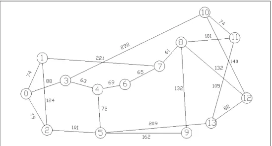
However, size of Model1 is very large, growing in the order of O(mn2), hence this approach is not applicable except for very small networks. For example, Model1 is formulated for a sample network topology (Figure (3.1)), obtained from [18], with 14 nodes and 21 edges. The optimal solution of this problem could not be found in 24 hours. Therefore we are going to examine if Model1 could be used for only one pair of vertices rather than for the entire graph.
CHAPTER 3. DIFFICULTIES IN MODELLING THE PROBLEM 20
Figure 3.1: 14-node network
3.2
Integer Linear Program For a Specific Pair
In Section (3.1), we have given Model1 to solve the problem for the entire graph and have seen that the size of Model1 is too large to be of practical use. Our experimentation has also confirmed that we can’t go beyond n ≥ 10. Here, we are going to formulate another ILP for a specific starting node s and terminating node t and will try to use it to find the optimal solution. New ILP will be referred to as Model2. Objective: Minimize X i∈N ri Subject to: X j:(i,j)∈A xijk− X j:(j,i)∈A xjik = 1, i=s; −1, i=t; 0, i 6= s,t; ∀i ∈ N, ∀k
wjk− ≥ wik+− M(1 − xijk) + cijxijk, ∀(i, j) ∈ A, ∀k
w+
CHAPTER 3. DIFFICULTIES IN MODELLING THE PROBLEM 21 w− ik ≤ Rmax, ∀i ∈ N, ∀k xij1+ xij2 ≤ 1 xij1+ xji2 ≤ 1 , ∀(i, j) ∈ A w−sk = wsk+ = 0, ∀k xijk ∈ {0, 1}, ri ∈ {0, 1} all variables ≥ 0
For a graph with n nodes and m edges, Model2, which includes only a specific pair, has 5n+4m variables and 6n+8m constraints. For example, in a graph with 32 nodes and 50 edges, Model2 would have 368 variables and 608 constraints. Al-though these numbers do not seem excessively large, our experimentation showed that Model2 is hard to solve and needs long solution times. Besides, restricting our attention to a pair of nodes at a time constitutes a major restraint for our problem. It is interesting to note that though the pairs are independent from each other, they are inter-related at the same time. Since an arc included in a path for pair (s1, t1) can also be used in a path for pair (s2, t2), the pairs are independent. However, if a regenerator is placed on node i for pair (s1, t1), it can be used for regeneration for pair (s2, t2), too. For this reason, the pairs cannot be considered separately, otherwise the solution for the entire graph may be sub-optimal, even though each solution for specific pairs is optimal.
We might still employ this formulation to find near optimal solutions nonethe-less. However, there is another major drawback of this model apart from its size and long solution times. This drawback will be explained in Section (3.3).
3.3
Problem With the Integer Linear Program
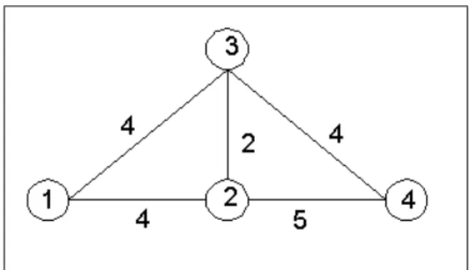
Let us look at the graph given in Figure (3.2). Say this graph represents a communication network with a degradation limit of 7, and we want to solve our problem on this network. Since the graph is very small, we can use Model1 to solve the problem.
CHAPTER 3. DIFFICULTIES IN MODELLING THE PROBLEM 22
Figure 3.2: A small example
Solution of Model1 tells us to place three regenerators on nodes 1, 2 and 3. In addition, Model2 can be used to solve the problem for the pair (1,4) and in the solution two regenerators are placed on nodes 2 and 3. Here one can see that there is a problem with the solutions of both Model1 and Model2. One and two regenerators are sufficient for the pair and for the entire network, respectively. For example, for pair (1,4) 1 → 3 → 4 could be selected as working path and 1 → 2 → 3 → 2 → 4 as the restoration path. With a regenerator placed on node 3, lengths of both paths will be within the degradation limit. In other words our models might end up in suboptimal solutions.
A critical point is that, both Model1 and Model2 will result in simple paths i.e. no vertices are repeated. Looking at constraints (3.3) and (3.4), it can be seen that if a path passes a node more than once, w+ik and wik− variables would have different values to take and they will take the largest value. This seems normal at first. Since the signal attenuates at every edge it passes, it is not logical to use a vertex or edge more than once. However, things get more complicated once we start thinking about regenerators on the paths.
Notice that, the restoration path in the optimal solution is a non-simple path. Since the signal is regenerated at node 3, it is better to select this non-simple path, which is longer than the simple path, rather than to place an additional regenerator on node 2.
CHAPTER 3. DIFFICULTIES IN MODELLING THE PROBLEM 23
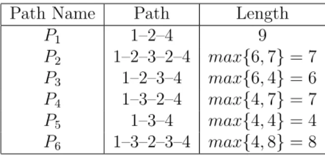
Table 3.1: Path lengths.
Path Name Path Length
P1 1–2–4 9 P2 1–2–3–2–4 max{6, 7} = 7 P3 1–2–3–4 max{6, 4} = 6 P4 1–3–2–4 max{4, 7} = 7 P5 1–3–4 max{4, 4} = 4 P6 1–3–2–3–4 max{4, 8} = 8
In the graph given in Figure (3.2) there are six different paths between pair (1,4). Assuming there is a regenerator on node 3, lengths of the alternatives are calculated. The paths and their lengths are given in Table (3.1).
With a degradation limit of 7, it is seen from Table (3.1) that all paths but P1 and P6 are feasible paths. This shows us that the paths in the feasible solutions do not have to be simple paths. Assuming, P2 is selected; some of the constraints of Model2 for this graph would be realized as follows.
r3 = 1 w+3 = 0 w1+= 0 w−2 ≥ 4 w+2 ≥ w2− w−3 ≥ w2++ 2 w+ 3 = 0 w−2 ≥ 2 w+ 4 ≥ w4− w−4 ≥ w2++ 5 These constraints imply that
w+
2 ≥ w2−≥ 4
w4−≥ 9
This means that, the length of P2 is 9 units, which is equal to the length of P1. In fact, it is smaller as seen from Table (3.1). But, Model2 has treated P2 as P1 and ignored the benefit we gained using the regenerator. This shows that Model2 is not appropriate to work with paths that are not simple. However, as just argued, there may be paths which are not simple but feasible. In addition, it may be
CHAPTER 3. DIFFICULTIES IN MODELLING THE PROBLEM 24
Table 3.2: Modified Graph with EC=2.
Original Graph Modified Graph
Vertices V = {1, 2, ..., n} V0 = {1, 2, ..., n, n + 1, ..., 2n}
Edges E = (i, j) E0 = (i, j) ∪ (i, j + n) ∪ (i + n, j) ∪ (i + n, j + n)
necessary to use those paths to find an optimal solution. Therefore, the model must be modified in order to handle non-simple paths.
3.4
Solution Approach to the Problem in
Model2
Since the model can examine only simple paths, we could try to modify the graph so that the paths that are not simple could be treated as simple paths. Our proposed modification is in fact, forming replicas of nodes and edges. The number of replicas we form is called; the expanding coefficient, which will be denoted as EC. For example, if we have two replicas along with the original node in the modified graph, then the expanding coefficient will be three.
First we want to study the case in which the expanding coefficient is two, which means we duplicate each node. The solution idea is that, if we duplicate each node, some non-simple paths will become simple paths since the path will visit the original node and then its duplicate node. This definition will be used later. By this way, each node is visited only once in the modified graph, although some nodes on the original graph are visited twice. If the nodes are duplicated, the edges must also be multiplied. We will represent the modified graph as G0(V0, E0)
and the corresponding directed network asGb0(N0, A0). The vertices and edges of
the original and the modified graph are shown in Table (3.2).
As it is seen from Table (3.2), we have an additional vertex for each vertex in
V . Since there are n vertices in V , vertices i and i + n represent the same vertex
CHAPTER 3. DIFFICULTIES IN MODELLING THE PROBLEM 25
Figure 3.3: a)Original Graph b)Modified Graph (EC=2)
with i0. In addition, to simplify our representation, we assume that (i0)0 is i, in
fact. This assumption is used to define the domains of the constraints. Similarly, we have four edges in the modified graph, instead of one original edge. By this way, using the modified graph as the input, the model we constructed is able to evaluate the paths in which some vertices are visited twice. Unfortunately, the size of the graph grows very fast. Now we have 2n vertices and 4m edges instead of n and m, respectively. To show how this modification changes a graph, original and modified versions of a simple graph are provided in Figure (3.3). As it is seen, although the original graph is very small, it becomes very complex after the modification.
3.4.1
Modified Integer Linear Program
ILP of the modified graph, which will be referred to as Model3 is very similar to Model2. The domains of the constraints and objective function are changed ac-cording to the modified graph. In addition, new constraints are added to Model2. Model3 is given and the new constraints are explained below:
CHAPTER 3. DIFFICULTIES IN MODELLING THE PROBLEM 26 Objective: Minimize X i∈N0 ri Subject to: X j:(i,j)∈A0 xijk− X j:(j,i)∈A0 xjik= 1, i=s; −1, i=s; 0, i 6= s,t; ∀i ∈ N0, ∀k w− ik ≥ w+ik− M(1 − xij) + cijxij, ∀(i, j) ∈ A0, ∀k w+ ik ≥ wik−− Mri, ∀i ∈ N0, ∀k w−ik ≤ Rmax, ∀i ∈ N0, ∀k
xij1 + xji1+ xij2+ xji2≤ 1
xij1+ xji1+ xij02+ xj0i2≤ 1 xij1+ xji1+ xi0j2+ xji02 ≤ 1 xij1+ xji1+ xi0j02+ xj0i02 ≤ 1 , ∀(i, j) ∈ A0 (3.7) w− sk = w+sk = 0, ∀k ri = ri0, ∀i ∈ N (3.8) xijk ∈ {0, 1}, ri ∈ {0, 1} all variables ≥ 0 In this formulation:
• Constraint (3.7) is a bit different from constraint (3.6). Since we have
expanded the graph, there is no need to use an edge of E0 more than once
in a path. Instead, we use the duplicate of that edge if necessary. Notice that the number of constraints used for disjoint paths gets bigger as EC increases.
• Constraint (3.8) is added to Model3. Since we have duplicated nodes, we
have now two nodes representing the same node. Therefore, if we have placed a regenerator on a node, this means we also have a regenerator on its duplicate node.
CHAPTER 3. DIFFICULTIES IN MODELLING THE PROBLEM 27
Figure 3.4: Rings in a path
Model3 has 10n + 16m variables and 17n + 48m constraints, in other words, its size is more than twice of the size of Model2. We have stated that, solving Model2 takes long time, naturally Model3 is harder to solve. For this reason, we have tried to find additional constraints to make the feasible area of the linear programming relaxation smaller without omitting integer feasible solutions. But before giving the constraints we will propose a theorem which will make the constraints valid.
Here, we want to make some definitions which will be used in the following theorems. The first one is the preference concept. Say there are two paths P1 and P2. If L(P1) ≤ L(P2) we say that P1 is preferred to P2 and show this with
P1 Â P2. The second one is the ring in a path. If each edge appears exactly once in the cycle portion of a non-simple path, then this portion is called a ring and the path is said to have a ring. For example, in the path f1∪ f2∪ f3∪ f4 of Figure (3.4) the cycle portion f2∪ f3 forms a ring. But the cycle portion f2∪ f2 of the path f1 ∪ f2∪ f2∪ f4 is not a ring.
It is obvious that a cycle in a path only occurs if there is a regenerator on the cycle. It seems it is possible to eliminate the rings of a path. In a ring, the path goes to the regenerator node through a sub-path, and comes back through another sub-path. It seems reasonable to use the same sub-path to go and come
CHAPTER 3. DIFFICULTIES IN MODELLING THE PROBLEM 28
back. This will be shown formally in the following Lemma.
Lemma 1 If there is a feasible s − t path P that has a ring, then there is always
another feasible s − t path P0 free of rings which is preferred to P .
Proof Look at the graph given in Figure (3.4). In this graph, s and t are the terminal vertices, j is the regenerator vertex and i is the vertex which is visited more than once. f1, f2, f3 and f4 are the path fragments between the vertices. The possible paths between pair (s, t) and their lengths are given in Table (3.3).
There are four possible cases:
1. L(P4) = lf1 + lf2 L(P2) = lf1 + lf2 ⇒ L(P2) ≤ L(P4) ⇒ P2 Â P4 2. L(P4) = lf1 + lf2 ⇒ lf1 + lf2 > lf3 + lf4 L(P2) = lf2 + lf4 ⇒ lf4 > lf1 ⇒ L(P3) = lf3 + lf4 L(P3) ≤ L(P4) ⇒ P3 Â P4 3. L(P4) = lf3 + lf4 L(P3) = lf3 + lf4 ⇒ L(P3) ≤ L(P4) ⇒ P3 Â P4 4. L(P4) = lf3 + lf4 ⇒ lf4 + lf4 > lf1 + lf2 L(P3) = lf1 + lf3 ⇒ lf1 > lf4 ⇒ L(P2) = lf1 + lf2 L(P2) ≤ L(P4) ⇒ P2 Â P4
Enumerating all possibilities, we see that there is always a path free of rings (P2 or P3) which is preferred to the one with rings (P4). With this Lemma we are able to eliminate paths with rings.2
Hence the following list of constraints can be incorporated into our model without eliminating the optimal solution.
CHAPTER 3. DIFFICULTIES IN MODELLING THE PROBLEM 29
Table 3.3: Rings in a path.
Path Name Path Path Length
P1 f1∪ f4 L(P1) = lf1 + lf4 P2 f1∪ f2∪ f2∪ f4 L(P2) = max{lf1 + lf2, lf2 + lf4} P3 f1∪ f3∪ f3∪ f4 L(P3) = max{lf1 + lf3, lf3 + lf4} P4 f1∪ f2∪ f3∪ f4 L(P4) = max{lf1 + lf2, lf3 + lf4} Additional Constraints: xijk ≥ xji0k, ∀(i, j) ∈ A (3.9) xijk+ xji0k ≤ rj + 1, ∀(i, j) ∈ A (3.10) X a:(a,j)∈A0a6=i0 xajk ≥ xi0j0k, ∀(i, j) ∈ A (3.11)
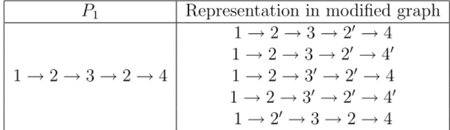
There are many alternative feasible paths in the modified graph. Although they are different in the modified graph, they represent the same path in the original graph. For example, for the graph given in Figure (3.2) assume that the working path, P1 is as follows, 1 → 2 → 3 → 2 → 4. Some of the paths which represent P1 in G0 are given in Table (3.4). In Table (3.4) there are five different paths, each of which represent the same path, P1 in fact. Besides, more paths, representing P1, could be found. It is obvious that, there is no need to allow this multi-representation case. It would be fine to prevent these additional paths, because omitting these additional paths will not result in losing feasible solutions for the original graph.
The arcs which are duplicates of the original arc are listed below and they are examined to identify which arcs can be selected under which conditions. The arc selection rules are as follows:
i → j This is the original arc of the graph. Therefore we prefer to use this arc,
if possible.
CHAPTER 3. DIFFICULTIES IN MODELLING THE PROBLEM 30
Table 3.4: Some of the paths which represent P1
P1 Representation in modified graph
1 → 2 → 3 → 20 → 4
1 → 2 → 3 → 20 → 40
1 → 2 → 3 → 2 → 4 1 → 2 → 30 → 20 → 4
1 → 2 → 30 → 20 → 40
1 → 20 → 3 → 2 → 4
i0 → j According to the preferences given above, a path visits a duplicate node
if the original node is visited before. Therefore, this arc can be used only if the path comes to node i0. In this case, we again prefer to go to the original
node using this arc.
i0 → j0 This arc goes from a duplicate node to another duplicate node. Therefore,
this arc is not used if arc (i0, j) or (i, j0) is available.
An edge can be on the simple part of the path which means this edge is used only once in the path or it can be on the cycle portion of the path meaning that the corresponding edge on the original graph is used twice. Edges used in a path on the modified graph can be divided into three types. If an edge is on the simple part then it is a type-I edge. Arc (i, j) is used if the edge is a type-I edge. If an edge is on the cycle portion of the path and if one of its terminating nodes is the regenerator node then this edge is a type-II edge. Type-II edges are used twice and used pair of arcs are (i, j) and (j, i0). If an arc is on the cycle portion and
does not have an end on the regenerator node then this arc is a type-III arc. In type-III edges, arcs (i, j) and (j0, i0) are used. Having defined the edge types, the
paths to be omitted are identified according to the following rules;
• Model3 is formulated for a specific pair of nodes. There is no need to
send the initial signal from duplicate of the source node instead of original source. This statement is valid for terminating node, too. Therefore, it is not necessary to duplicate starting and terminating nodes and related edges.
CHAPTER 3. DIFFICULTIES IN MODELLING THE PROBLEM 31
• Constraint (3.9) is used for type-I edges. If an edge on the path is type-I
edge then only arc (i, j) could be used to represent this edge.
• Constraint (3.10) is used for type-II edges. Both arc (i, j) and arc (j, i0) can
be used only if the edge is a type-II edge. This constraint uses variable ri
to identify whether the edge is a type-II edge or not.
• Constraint (3.11) is used for type-III edges. Arc (i0, j0) is used if edge {i0, j0}
is a type-III edge. If there is another entrance to node j0, which means the
node is visited more than once resulting in the edge is a type-III edge. Notice that we do not omit any feasible solutions from the original integer solution set using these additional constraints.
As it is said before, we are examining a special case where EC=2. Therefore solution of Model3 will be optimal only if all the feasible paths visit each node twice at the most. Otherwise, some feasible solutions and possibly the optimal solution might be ignored. This means, if there is a node which is visited three or more times in a feasible path, there would be a problem again. Now we want to discuss the optimality of solutions of Model3 for different EC values, first.
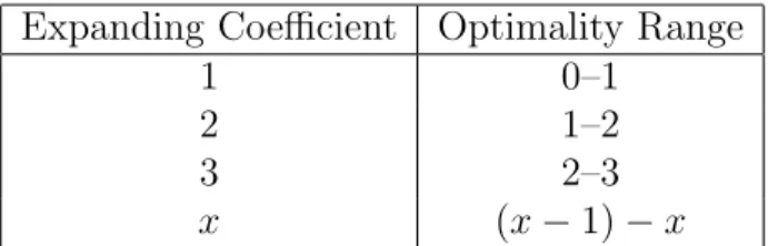
A node is visited more than once only if there are regenerators placed on the graph. To be more exact, it can be said that a signal visits a node twice if there is one regenerator, visits three times if there are two regenerators etc. . . Otherwise, there is no need to visit those nodes more than once. Therefore an optimality range can be defined here, and we can say that a solution for a given EC value is optimal if the solution is in related optimality range. Optimality ranges are given in Table (3.5).
Having defined the optimality range, we can explain the procedure to find optimal solution for a given pair using ILP formulation. First, Model2 is formu-lated for EC =1 and solved. If the result is in optimality range, it is optimal. Otherwise, increase EC by one, solve again. Continue this procedure until the solution is within the optimality range.
CHAPTER 3. DIFFICULTIES IN MODELLING THE PROBLEM 32
Table 3.5: Optimality Ranges. Expanding Coefficient Optimality Range
1 0–1
2 1–2
3 2–3
x (x − 1) − x
that, whenever a node is to be visited three or more times in a feasible path P , there is always another path P0 that can be preferred to P and on which each
node is visited at most twice, we can conclude that EC=2 case does not ignore the optimal solution.
Theorem 3.4.1 If there is a feasible s − t path P that visits a node more than
twice in a graph G, then there is always another feasible s − t path P0 which visits
a node at most twice and is preferable to P .
Proof Look at the graph given in Figure (3.5). In this graph, s and t are the terminal vertices, j and k are the regenerator vertices and i is the vertex which is visited more than twice. f1, f2, f3 and f4 are the path fragments between the vertices. The possible paths between pair (s, t) and their lengths are given in Table (3.6). Notice that, using Lemma (1), some other possible paths with rings can be discarded.
There are three possible cases and in each case there are two more possibilities for the lengths of the path fragments:
1. L(P3) = lf1 + lf2 ⇒ lf1 > lf3 lf1 + lf2 > lf3 + lf4 (a) L(P1) = lf1 + lf2 ⇒ P1 Â P3 (b) L(P1) = lf2 + lf4 ⇒ lf4 > lf1 ⇒ L(P2) = lf3 + lf4 ⇒ P2 Â P3 2. L(P3) = lf2 + lf3 ⇒ lf3 > lf1 lf2 > lf4
CHAPTER 3. DIFFICULTIES IN MODELLING THE PROBLEM 33
Figure 3.5: Visiting a vertex more than twice
Table 3.6: Multi visited vertices.
Path Name Path Path Length
P1 f1∪ f2∪ f2 ∪ f4 L(P1) = max{lf1+ lf2, lf2 + lf4} P2 f1∪ f3∪ f3 ∪ f4 L(P1) = max{lf2+ lf3, lf3 + lf4} P3 f1∪ f2∪ f2∪ f3 ∪ f3∪ f4 L(P3) = max{lf1 + lf2, lf2 + lf3, lf3 + lf4} P4 f1∪ f3∪ f3∪ f2 ∪ f2∪ f4 L(P4) = max{lf1 + lf3, lf3 + lf2, lf2 + lf4} (a) L(P1) = lf1 + lf2 ⇒ P1 Â P3 (b) L(P1) = lf2 + lf4 ⇒ lf4 > lf1 ⇒ L(P2) = lf3 + lf4 ⇒ P2 Â P3 3. L(P3) = lf3 + lf4 ⇒ lf4 > lf2 lf3 + lf4 > lf1 + lf2 (a) L(P1) = lf1 + lf2 ⇒ P1 Â P3 (b) L(P1) = lf2 + lf4 ⇒ lf4 > lf1 ⇒ L(P2) = lf3 + lf4 ⇒ P2 Â P3
According to Theorem (3.4.1), we can conclude that modification of the graph with EC =2 is sufficient to solve the problem. 2