Modeling location-allocation of military items to the depots without branch classification

MODELING LOCATION-ALLOCATION OF

MILITARY ITEMS TO THE DEPOTS

WITHOUT BRANCH CLASSIFICATION

A THESIS

SUBMITTED TO THE DEPARTMENT OF INDUSTRIAL

ENGINEERING

AND THE INSTITUTE OF ENGINEERING AND SCIENCES

OF BILKENT UNIVERSITY

IN PARTIAL FULFILMENT OF THE REQUIREMENTS

FOR THE DEGREE OF

MASTER OF SCIENCE

By

Ali Sezgin Işılak

JUNE, 2002

I certify that I have read this thesis and in my opinion it is fully adequate, in scope and in quality, as a thesis for the degree of Master of Science.

Assoc. Prof. Osman Oğuz (Principal Advisor)

I certify that I have read this thesis and in my opinion it is fully adequate, in scope and in quality, as a thesis for the degree of Master of Science.

Assoc. Prof. İhsan Sabuncuoğlu

I certify that I have read this thesis and in my opinion it is fully adequate, in scope and in quality, as a thesis for the degree of Master of Science.

Asst. Prof. Oya Karaşan

Approved for the Institute of Engineering and Sciences

Prof. Mehmet Baray

III

ABSTRACT

MODELING LOCATION-ALLOCATION OF

MILITARY ITEMS TO THE DEPOTS

WITHOUT BRANCH CLASSIFICATION

Ali Sezgin Işılak

M.S. in Industrial Engineering

Advisor: Assoc. Prof. Osman Oğuz

June 2002

This thesis shows how Turkish Land Forces can optimally combine its distribution efforts and repositions the items in the existing distribution network after the merging of Ordnance, Signal, and Engineers Corps and their resources as a single unit. A mixed integer programming model is proposed, and for the implementation of the model, optimization modeling software GAMS is used. The model is implemented for two stock level choices (120-day and 180-day basis) with taking safety stock constraints into account, which are determined by Logistic Command. How distribution costs are affected by the number of open depots is investigated, and ideal number of depots and their locations in distribution network are proposed.

Keywords: Mixed integer Programming, Location-Allocation, Distribution Costs, Safety Stock, Capacitated Facility Location.

ÖZET

ASKERİ MALZEMELERİN

SINIF FARKI GÖZETİLMEKSİZİN

DEPOLARA TAHSİSİNİN MODELLENMESİ

Ali Sezgin Işılak

Endüstri Mühendisliği Bölümü Yüksek Lisans

Tez Yöneticisi: Doç. Dr. Osman Oğuz

Haziran 2002

Bu çalışmanın amacı, Türk Kara Kuvvetlerinin Ordudonatım, Muhabere, İstihkam sınıflarını ve bu sınıflara ait depoları nasıl en faydalı şekilde tek birim olarak birleştirebileceğini ve yeni sistemde malzemeleri varolan dağıtım ağı içerisinde nasıl yerleştirebileceğini göstermektir. Tamsayılı programlama modeli önerilmiş ve bu modelin uygulanması için GAMS yazılımı kullanılmıştır. Model Lojistik Komutanlığı tarafından belirlenmiş emniyet stoklarıyla ilgili kısıtlar gözönüne alınarak iki stok seçeneğine göre (120 ve 180 günlük stok seviyesi) çalıştırılmıştır. Dağıtım masraflarının açık depo sayısıyla nasıl etkilendiği sorusuna yanıt bulunmaya çalışılmış ve ideal açık depo sayısı ve yerleri önerilmiştir.

Anahtar Kelimeler: Tamsayılı Programlama, Konum-Tahsisat, Dağıtım Masrafları, Emniyet Stoğu, Kapasite Kısıtlı Tesis Yerleşimi.

V

ACKNOWLEDGEMENT

I would like to express my deep gratitude to Dr. Osman Oguz and Dr. İhsan Sabuncuoğlu for their guidance, attention, understanding, and patience throughout all this work.

I am indebted to the reader Dr. Oya Karaşan for her effort, kindness, and time.

I would like to thank Major Tayfun Kıllıoğlu for his corrections and Major Mehmet Pınar, Captain Erol Çetin for their understanding and support during the collection of data.

I would like to thank all Industrial Engineering Faculty, staff and my friends for their assistance and support during the graduate study.

Finally, I am very thankful to my family and fiancee for their support, tolerance and patience.

VII

CONTENTS

List of Figures X List of Tables XI

Definitions XII

English-Turkish Meanings of Some Military Terms XIII

1. INTRODUCTION 1

1.1. Land Forces Inventory System 5

1.1.1. National Stock Number 5 1.1.2. Stock Policy of Land Forces 6 1.1.3. Provision Types of Land Forces 6 1.1.4. Old, Current and Proposed Depot Location Policies 8

2. LITERATURE SURVEY

12

2.1. US Navy Inventory System 14

2.2. Studies of Civilian Distribution Networks 15

2.3. Aggregation in Network Studies 18

3. ANALYSIS OF THE PROBLEM and MATHEMATICAL

FORMULATION

20

3.2. Assumptions 24

3.2.1. All Demands Must be Satisfied 24 3.2.2. All Costs are Known and Remain Fixed 24 3.2.3. Availability of Each Depot to Every End User 25 3.2.4. Any Demand Point can be Supplied From More Than One Depot 25 3.2.5. Unchanging Demand Point Location 25

3.3. Formulation 25

3.3.1. Indices 25 3.3.2. Initial Data and Parameters 26 3.3.3. Variables 26 3.3.4. Constraints 26 3.3.4.1. Demand Constraint 26 3.3.4.2. Capacity Constraint 26 3.3.4.3. Location Constraints 28 3.3.4.4. Safety Stock Constraints 29 3.3.4.5. Non-Negativeness and Binary Variables 31 3.3.5. Objective Function 31

3.4. Experimentation 32

3.5. Results 35

3.5.1. Location-Allocation of Depots When GDLS is Taken as 120 Day 35 Basis

3.5.2. Location-Allocation of Depots When GDLS is Taken as 180 Day 38 Basis

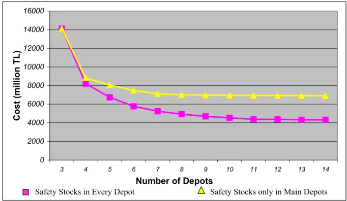
3.5.3. Effect of Allocation of Items Without Safety Stocks in the Main 41 Depots

4. CONCLUSION

43

IX

Bibliography

47

Appendix

A. Data File 50

B. Number of Items in the Depots for 120 Day Based Stock Level 59

List of Figures

Figure 1.1. National stock number 5 Figure 1.2. Stock policy of items, which are required frequently by the military 6 units.

Figure 1.3. Old distribution policy. 8 Figure 1.4. Current distribution policy. 8 Figure 1.5. Proposed distribution policy. 9 Figure 1.6. Safest region for keeping safety level of supply for unexpected battle

conditions. 10 Figure 2.1. Relationship between service/cost performance and number of

warehouse locations. 13 Figure 3.1. Utilization of depots with 14 depots. 35 Figure 3.2. Utilization of depots with three depots. 36 Figure 3.3. Restricting the maximum number of depots (M) for the 120-day based stock level. 36 Figure 3.4. Utilization of depots when restricting the number of depots to four

depots. 37 Figure 3.5. Utilization of depots when restricting the number of depots to seven

depots. 37 Figure 3.6. Utilization of depots with 14 depots. 38 Figure 3.7. Restricting the maximum number of depots (M) for 180-day based

stock level. 39 Figure 3.8. Utilization of depots when restricting the number of depots to six

depots. 40 Figure 3.9. Utilization of depots when restricting the number of depots to ten

depots. 40 Figure 3.10. Restricting the maximum number of depots (M) without safety stock

constraints for 120-day based stock level. 41 Figure 3.11. Restricting the maximum number of depots (M) without safety stock

XI

List of Tables

Table 3.1. Location and capacities of the depots. 22 Table 3.2. Transportation costs. 24 Table 3.3. Required CPU times and number of iterations for 120-day stock level. 33 Table 3.4. Required CPU times and number of iterations for 180-day stock level. 34 Table A.1 Weights and covered areas of each item. 50 Table A.2 Shortest distances between depots and demand points (in kilometers). 51 Table A.3 Shortest distances between depots and demand points (in kilometers). 52 Table A.4 Demand data for 180-day based stock level. 53 Table A.5 Demand data for 180-day based stock level. 54 Table A.6 Demand data for 180-day based stock level. 55 Table A.7 Demand data for 180-day based stock level. 56 Table A.8 Demand data for 180-day based stock level. 57 Table A.9 Demand data for 180-day based stock level. 58 Table B.1 Allocated number of items in each depots for 120-day based stock level with 4 open depots. 59 Table B.2 Allocated number of items in each depots for 120-day based stock level with 7 open depots. 60 Table B.3 Allocated number of items in each depots for 120-day based stock level with 14 open depots. 61 Table B.4 Allocated number of items in each depots for 120-day based stock level

with 14 open depots. 62 Table C.1 Allocated number of items in each depots for 180-day based stock level with 6 open depots. 63 Table C.2 Allocated number of items in each depots for 180-day based stock level

with 10 open depots. 64 Table C.3 Allocated number of items in each depots for 180-day based stock level

with 14 open depots. 65 Table C.4 Allocated number of items in each depots for 180-day based stock level

DEFINITIONS

Logistics (military): The science of planning and carrying out movement and

maintenance of forces, dealing with design and development, acquisition, storage, movement, distribution, maintenance, evacuation and disposition of material; movement, evacuation and hospitalization of personnel; acquisition or construction, maintenance, operation and disposition of facilities; and acquisition or furnishing services.

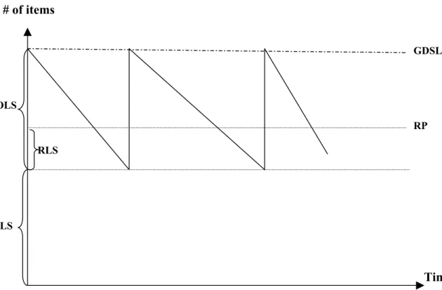
Operating Level of Supply (0LS): is the required amount of stock (number of days’

supply) for supplying military units.

Request Level of Supply (RLS): is the required amount of stock (number of days’

supply) for satisfying demands between time of making an order and delivery time of items.

Safety Level of Supply (SLS): is the minimum amount of stock (number of days’

supply) that should be kept to serve as a buffer against unexpected shipment delays or major fluctuations in demand.

Reorder Point (RP): is the quantity to which inventory is allowed to drop before a

replacement order (fill-in) is placed. Reorder point equals to the sum of request level of supply and safety level of supply.

Goal Demand Stock Level (Storage Objective) (GDSL): is the amount of stock

(number of days’ supply) that is calculated as a sum of operating level of supply and safety level of supply. This stock level is only applied to the items that are demanded more than four times in a year by the military units.

XIII

Maintenance Safety Stock Level (MSSL): is applied to the items that are requested

less than four and more than one times in a year by the military units. These items kept in stock as the half of the goal demand stock level.

Excess Stocks (ES): is applied to the items that are not demanded frequently. If an item

is defined as an excess stock then logistic unit or depot will send this item back to the main depots, which are located in Central-Anatolia.

Recoverable Stock Items (RSI): items that can be repaired in the local regions.

ENGLISH-TURKISH MEANINGS OF SOME MILITARY TERMS

Turkish Land Forces: Türk Kara Kuvvetleri Corps: Kolordu

Brigade: Tugay

Branch: Askeri sınıf (Ordudonatım, muhabere, vb.) Ordnance Corps: Ordudonatım sınıfı

Signal Corps: Muhabere sınıfı Engineers Corps: İstihkam sınıfı Quartermaster Corps: Levazım sınıfı Subordinate Units: Bağlı birlikler Headuarters: Karargah

CHAPTER 1

INTRODUCTION

The mission of Land Forces Logistics System is to provide effective weapons, vehicles and forces and then maintain sustained support to them in war and piece conditions with minimum expenditure of resources.

The standard operating procedures and business processes of the logistics units of Turkish Land Forces are very outdated and incompatible with current technology. Considering the cost of the materials that are being used for the special military purposes, the burden of this on the budget is considerably high, and certain measures must be taken for reengineering of the logistics units.

In the recent years, Turkish Land Forces have started many projects about logistics to catch up with technological trends. In 1986, Turkish Land Forces redefined its logistics concept, and decided to establish a unit which will manage all logistics efforts of all branches. For this purpose, Logistic Command was established in 1988.

In 1990, Material Management Centers were established for each of the branches in Logistic Command. Also main depots and forth-level depots began to use computers. Thus, main depot management is now able to keep track of the number of items in its subordinate depots in corps’ region.

In 1996, Turkish General Staff has started “Continuous Acquisition and Life Cycle Support (CALS)” project, which aims to create a shared information environment wherein information is shared freely across the military organizations. The intent of CALS is to improve the timeliness, reduce the cost, and improve the quality of defense system acquisition and support. It also provides supply chain integration for the suppliers. CALS (in other terms Commerce

At Light Speed) is also an ongoing project at NATO to support co-operation in NATO on logistics, with a focus on meeting war fighter requirements for operational interoperability.

In 2000, Turkish Land Forces evaluated the results of former studies and updated the logistics concept, and then launched the Logistics Information Systems Project. For the execution of projects, Turkish Land Forces established Logistics Information Systems Center (LISC), which is formed by officers from all branches. LISC’s mission is to determine the requirements of the system by cooperating with officers in Logistic Command and depots. It also started to collect statistical data that is need for execution of projects. If needed, LISC can work with Havelsan and other civilian firms for developing algorithms, executing projects, and developing software to be used in logistics management and control.

In 2001, Turkish Land Forces developed The Joint Support Concept. The aims of the concept include:

i. To combine ordnance, signal, engineer, quartermaster corps under one unit to provide

cooperative purchase, sharing depot resources and combining transportation efforts. All logistics processes will be managed from one center. Items will be technically grouped and allocated to the depots rather than allocation as a branch classification. As an example; all logistics corps were purchasing wheels separately, which is more costly than cooperative purchase. Now all of them send their needs to the Ordnance Corps and Ordnance Corps use a bidding system for purchasing wheels (providing quantity discount). But this is still not the case for many of the items.

ii. Each item will be bar-coded and required computer network will be installed for the visibility of items in the system. The existing logistics system infrastructure does not meet the requirements of the dynamic structures of military units due to lack of control on all over the system. Immediate asset visibility could increase exponentially the accuracy and quickness of re-supply to the military units. Visibility of items includes; item movements in logistics

process, required minimum stock level for each item, shelf life, provision and expiration times of items.

iii. Brigades will store the items at a minimum level sufficient only for preventing shortages until the next order come to the brigade. So, procurement lead times gain more importance and requests should be sent in shorter times.

iv. To reduce spare and repair parts storage and holding costs by consolidating or disposing of inventory that is needed to meet current operating and strategic battle reserve requirements. Life cycle cost analyses of the items will be made and storage objectives of each item redefined after these analyses.

v. For providing military units to move quickly and especially in state of war supplying required item to the military units rapidly, mobile stocks (for example vehicles that carry containers) will be formed.

Again in 2001, for a pilot Logistics Information Systems Project, two brigades were selected. Logistics units of these brigades were computerized and began to request their demands on-line directly from main depots and their demands were sent only from the main depots.

Since January 2002, for facilitating automation and minimization of stock level, storing duties of fourth level depots were terminated. Fourth level depots are located in corps region for each of the logistics branches and former duty of these depots was to meet the demands of the corps subordinate units. The maintenance sections of these depots are still active, which have maintenance duty of recoverable items that are economical to repair. Main depots began to directly meet the demand of brigades and its superiors, except Ordnance Corps. By the end of the 2002, Ordnance Corps will also start to meet the demands of brigades directly from its main depot.

In 2003, Turkish Land Forces will make an evaluation of situation in the light of collected statistical data, and results of the applications. Between the years 2003-2005, Turkish Land Forces will continue to develop new computer programs, and all items will be bar-coded and have visibility in all stages of the logistics process.

By the year 2005-2010, Turkish Land Forces want to implement a new support concept, which is called “Force 2010”. All branches will be united and all resources of these branches will be used jointly.

The goal of all these efforts are to provide highest effectiveness, maximum readiness for battle conditions and while doing this, keeping logistics costs at minimum level in peace conditions. Responsiveness to the requirements of the troops in a battlefield and also in peacetime is an important factor for their survival.

The resources, techniques, and methods are required for preserving, packaging, transporting, loading and unloading, storing material systems, their support equipment, basic sustainment material (for example, batteries, lubricants), and associated supplies of all classes. These should include the procedures, environmental considerations, and equipment preservation requirements for both short and long-term storage.

There must be standardization in all levels of logistics support; for example, when one employee takes a request, it takes only few minutes to prepare the required documents, but then these documents can wait for one week in a queue on a desk in the process (maybe only for approval). Manual workflow cycle time varies from unit-to-unit, place-to-place, and employee-to-employee in the system. As a result the response time varies a lot, and it may take months to deliver an item. If reengineering and automation efforts are applied to processes then there will be no delays. The people who do the work should make decisions and management should handle any exceptions. Then the number of requests handled can be increased a hundred times.

In the present system the flow of materials is usually top down in other words superior to subordinate. Obsolete materials are being stocked “in case of need”. The new system can detect obsolete materials in stock, and facilitate their transfer to the needed accountancies or back to the main depots.

1.1. LAND FORCES INVENTORY SYSTEM

The Land Forces Inventory System’s organization is similar in many ways to that of large companies that provide goods and services to customers in the private sector with one difference; it must also take into account readiness for battle conditions. The primary goal of both the Land Forces Inventory System and that of the private sector is to satisfy customers. The Logistics Command manages the Land Forces Inventory System.

1.1.1National Stock Number

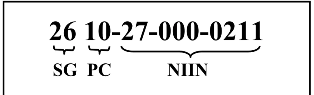
Every item within the inventory system has a unique National Stock Number, a 13-digit code. The first four digits denote supply class, and the last nine digits give the National Item identification number. The supply class breaks into two parts. The first two digits indicate the supply group that identifies the major item category (for example, 26 tires and 28 engines and their components), other two digits define the product class of item in that supply group (for example, 2640 tires repair tools, 2815 diesel engines and their components).

Figure 1.1. National Stock Number

26 10-27-000-0211

Depots are formed from many buildings whose sizes and properties are different from each

other. Items, which have the same supply group number in their national stock number, are located in the same conditions and places in the depots. National stock number also provides a basis for bar-coding process.

1.1.2 Stock Policy of Land Forces

The figure below summarizes the general stock policy for each item in the land forces:

# of items

Figure 1.2. Stock policy of items, which are required frequently by the military units (For abbreviations look at the definitions section).

1.1.3 Provision Types of Land Forces

There are mainly two types of provision in military:

Pull System: Provision is provided when a demand occurs (such as breakdown of tank’s

shock absorber). Time GDSL RP OLS RLS SLS

demand items

Logistic Command determines stock level by evaluating the actual demand of the past year requirements. But when number of item decreases to RP level, a new order is placed.

Push System: Provision is provided periodically. For example; spark plug of an armored

carrier is a spare part that should be changed in each six months or after 4000 km. Generally, first condition is applied in peace. To determine stock level, the formula below is used:

GDSL = X * Y * 360 (days)

Length of cycle period for maintenance (days)

where X is the number of the main system (for example; total number of armored carrier or G-3 rifle in the land forces), Y is the number of required items that will be exchanged for maintenance of main system in one period (for example; eight spark plugs are exchanged for the armored carrier in every six month). Logistic Command makes plans to send items to the brigades periodically.

BRIGADE Items are sent periodically DEPOT

Both of the two policies are currently in use, but there are some problems in the application

of the push system. Periodical demand of the items is still determined mostly by manual process, which causes delays in supplying efforts, sometimes the required item is never sent. The lack of trust of the people in the logistics system brings about informal processes, which harm the system and culture of the organization.

Logisticians, who are responsible from logistics process in brigades, continuously send requests to depots for items, which should be sent by a push system without requests. They want to keep more storage than there should be, as an hedge against system faults. And these

DEPOT BRIGADE

informal requests bring much work to the management of depots and Material Management Centers in Logistics Command. Thus, it causes more system faults in distribution. Consequently life cycle analysis of each item and automation are required as soon as possible to apply the push system and to decrease the level of illegal stocking in military units, which brings high costs to the system.

1.1.4 Old, Current and Proposed Depot Location Policies:

Figure 1.3. Old distribution policy.

The figure above represents the old system. At first, all items come to the main depot and then it only supplies distribution depots. Distribution depots represent the depots that are located in corps region and they only supply corps’ subordinate units. This system is myopic, very time consuming and costly. Each unit has its own stock levels. Thus system requires more items to hold in stock in order to keep the system operational. While one depot has an excess of materials, another depot may be out of stock for those materials.

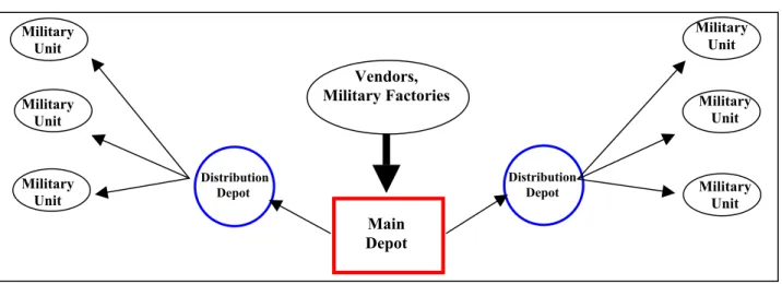
Figure 1.4. Current distribution policy.

Distribution Depot Distribution Depot Main Depot Military Unit Military Unit Military

Unit Military Unit

Military Unit Military Unit Vendors, Military Factories Military Unit Military Unit Military Unit Military Unit Military Unit Military Unit Main Depot Vendors, Military Factories

Since the beginning of 2002, a new distribution policy depicted in Figure 1.4 is in the process of being put into use. There is only one main depot at the center of the country, which has all related items. All logistics branches store inventory in its subordinate main depot. Its location is ideal for safety reasons, and having a single depot makes controlling the stock level very easy. Management of depots can be simplified and stock levels can be decreased by making use of total resource visibility. Also, bar-coding process can be implemented more easily. On the other hand, transportation costs and delivery times for supplying units are increased. The needed depot capacities can be insufficient for required stocks and this requires building new depot sections, which will bring high costs. If the main depot is destroyed then all the stock of that logistics branch will be lost. To balance and curtail these disadvantages, a third alternative is proposed by LISC as shown in Figure 1.5.

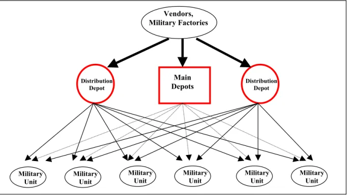
Figure 1.5. Proposed distribution policy.

The main objective of this thesis is to optimize and evaluate this proposed system. LISC wants to test the idea of using the depots that are located in corps region and apply the same automation procedures to these depots, and manage all these depots from one center without logistics branch classification. All logistics corps will be united and the system will have one stock level. By the help of automation, when a demand occurs, the system will decide to send

Military Unit Distribution Depot Distribution Depot Main Depots Vendors, Military Factories Military Unit Military Unit Military Unit Military

the item from the closest depot, which include that item in its inventory. This will decrease stock level, ensure readiness and decrease procurement lead times. The majority of the units are close to the borders, therefore system automatically will use the main depots as a last choice due to the minimization of cost and time. This proposal claims that if only main depots are used for meeting demands it will be very costly and system can’t achieve required procurement lead times.

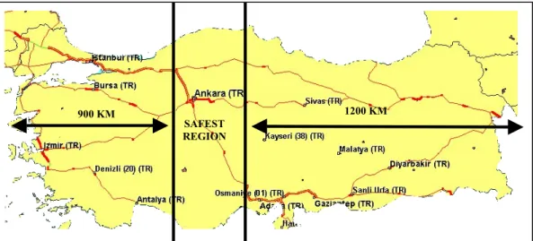
Turkey is located geographically in a very unstable region. Land Forces Command wants to locate the safety level of supplies in main depots that are located in Central-Anatolia, which is equally distanced to all other regions, and can supply all units. Therefore, it can also satisfy the security need for battle conditions.

Figure 1.6. Safest region for keeping safety level of supply for unexpected battle conditions.

If stock level decreases to the safety level of supply for any item, that item no longer will be sent to the demand points until the new order has been received by the depots. These items can stay in the main depots for a very long time that means, maintenance should be provided. The fourth level depots will be only used for operating level of supply, so that maintenance will not be required in those depots. There are nearly 300000 kinds of items in the Turkish Land Forces inventory. Consequently Logistic Command wants to locate any supply group only in one of the main depots. Otherwise required vehicle and tools must be kept for every item in each main depot and maintenance personnel should be increased, which will bring

SAFEST REGION

high costs. For preventing obsolescent materials in inventory, main depots must send items to the demand points from their inventory with “first come first out (FIFO)” principle.

Now, it is time to take strategic decisions for how to unite logistic corps, which depots should be used in distribution network, how items should be allocated to the depots for minimization of distribution costs and procurement lead times.

In this thesis, our goal is to investigate how the distribution costs are affected when the existing fourth level depots are used for stocking, and also after satisfying security conditions how much room should be allocated for each of the items in every depot. We have developed a mixed-integer programming model for solving this problem. The model determines which of the available depots will be in use, and assigns items to depots, thus specifying distribution channels for all items. Its objective is to minimize the operating costs of the depots and total transportation costs. The model is solved for two alternative operating policies:

a) 120-day based stock level b) 180-day based stock level

CHAPTER 2

LITERATURE REVIEW

The Council of Logistics Management, which is a non-for-profit professional association for people interested in logistics management in USA, defines logistics as the process of planning, implementing and storage of raw materials, in-process inventory, finished goods and related information from point of origin to point of consumption for the purpose of conforming to customer requirements (Kasilingam, 1998).

One of the strategic decisions in logistics is determining where to locate facilities and how to allocate the demand to the selected facilities considering their capacities. The goal in evaluating warehouse network structure is to determine the network configuration (i.e., the number, size, location, and service regions of warehouses) that provides a required level of customer service at minimum operating cost. In an effort to maintain superior distribution performance, companies periodically reconfigure their warehouse networks to respond to changing business requirements. A survey shows that if a company had not looked at its distribution system for more than four years, it could well be paying 200 percent more than that is necessary (Cooper, 1990).

While taking strategic decision for new location of facilities, organizations must treat geographically dispersed resources as though they were centralized. The conflict between centralization and decentralization is that decentralizing a resource gives better service to those who use it, but at the cost of abundance and missed economies of scale. Companies no longer have to make such trade-offs. They can use databases, telecommunication networks, and standard processing systems to realize the benefits of scale and coordination while maintaining the benefits of flexibility of service.

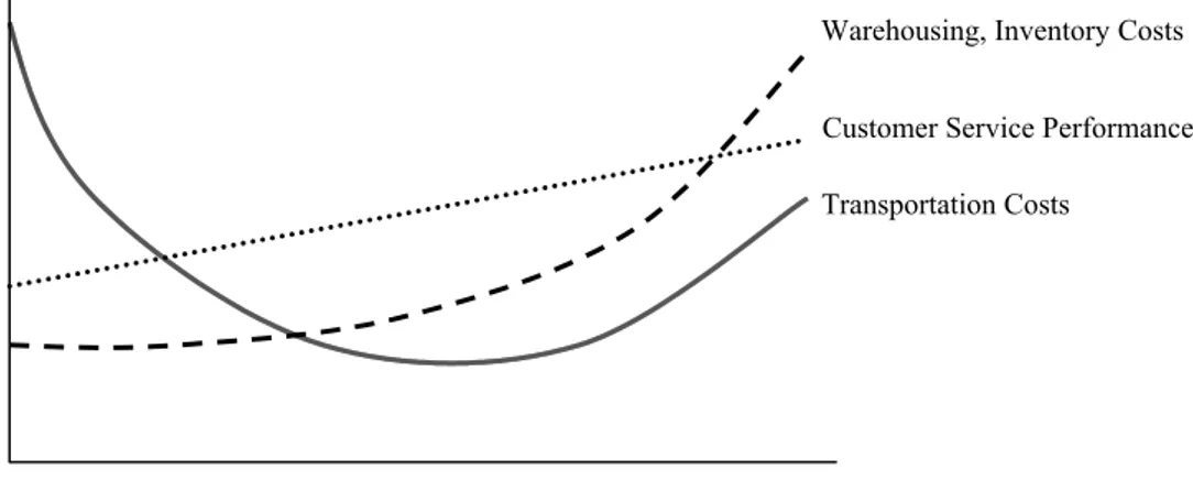
Increasing the number of warehousing facilities in a logistic network generally improves customer service, because, additional stocking locations reduces average delivery times to customers. However, more warehouses increase warehousing and inventory costs. Inventory costs increase because a greater number of warehouses means that more safety level of supply inventory must be held system-wide to provide specified level of customer service.

In contrast transportation costs decrease as the number of facilities increase over some range. This transportation cost advantage becomes diminished, however if too many warehouses are present because the shipment sizes between supply points and warehouses decrease to the point where there is little shipment consolidation advantage over direct shipment to customers (Robeson & Copacino, 1994)

Figure 2.1. Relationship Between Service/Cost Performance and Number of Warehouse Locations.

Facility location problems form an important class of integer programming problems, with applications in the telecommunication, distribution and transportation industries. When each facility has a limited capacity, then the problem is called capacitated facility location problem.

Customer Service Performance

Number of Warehouses

Warehousing, Inventory Costs

2.1. US Navy Inventory System

The inspiration to combine all the branches in Turkish Land Forces and to manage all inventory from one center was prompted by the examples in other countries, especially the US Navy. US Navy forms a model for integration of all classes in Turkish Land Forces. The integration of inventory management for all military branches date back to World War II when USA’s huge military expansion required the rapid procurement of great amounts of munitions and supplies. All branches began to systematically buy, store and issue items through the Defense Logistic Agency.

On October 2, 1995, the Navy Inventory Control Point (NAVICP) was established with the merging of the former Aviation Supply office in Fhiladelphia and Ships Parts Control Center in Mechanisburg. The purpose of this merger was to bring together all of the Navy’s Program Support Inventory Control Point functions under a single command. NAVICP is the sole controller of navy wholesale inventory and responsible for over 350,000 items of supply, $15.5 billions of inventory. It has to position its inventory optimally (in 22 Defense depots worldwide) to fulfill customer demand on time. There are many projects and studies about NAVICP. Two of them are most related with our study and deal with optimizing positioning of Navy wholesale inventory.

The first of these projects is described in Reich (1999). Reich developed an integer linear program that positions depot level repairable line items to achieve minimum distribution time subject to cost and other determined constraints. His extensive analysis of the distribution network indicated the Navy can cut response time and distribution cost by better strategic positioning of wholesale inventory within the existing network. He also proposed, cutting costs by increasing the use of Premium Transportation Facility that is owned by the Army. To solve the model, he used 57 representative recoverable stock items in his model, which inspired us to select representative items from each branch for simplicity of our model.

The second study is presented by Kaplan (2000), who developed a heuristic algorithm that optimally positions line items to serve historical requisitions by Naval units over an 18-month period. Repositioning minimizes distribution costs subject to constraints on customer wait time and depot capacities. A distribution scheme is modeled for 32,521 unique wholesale items from 22 depots to 126 aggregated customer regions worldwide. He found that Navy can reduce distribution cost by better strategic positioning of Navy’s inventory within the existing distribution network. And he also proposed that Navy can also achieve savings by positioning stocks at just a few locations, rather than at many, and by positioning items together in aggregate product groups, a policy that is widely accepted in logistics.

Kaplan showed the effect of the number of open depots on the distribution costs in his study. Following this line, we also carried out some analysis on the relation between number of depots and total system cost using our model. We were able to make recommandations about the reasonable number and locations of the depots.

2.2. Studies of Civilian Distribution Network:

Pirkul and Jayaraman (1998) presented a mixed integer programming model, PLANWAR, for the multi-commodity, multi-plant, capacitated facility location problem that seeks to locate a number of production plants and distribution centers so that total operating costs for the distribution network are minimized. And they developed an efficient heuristic solution procedure for this supply chain management problem which is basis on Lagrangian relaxation.

Murray and Gerrard (1998) presented a study on Capacitated Regionally Constrained p-median problem for siting service facilities, which incorporates regional requirements in a location-allocation framework, in addition to ensuring that maximum capacity limitations are maintained. We used similar constraints in the formulation of our model.

Holmberg, Ronnqvist, and Yuan (1999) described a new solution approach for the capacitated facility location problem in which customer is served by a single facility. A primal heuristic, basis on a repeated matching algoritm which essentially solves a series of matching problems until certain convergence criteria are satisfied, is incorporated into the Lagrangian Heuristic. Finally, a branch and bound method, basis on the Lagrangian heuristic is developed and it is found that method computationally more efficient than the commercial code CPLEX. Lagrangian Heuristic terminates with either proved optimality or a fairly small gap so it can be said that method is more useful for diffucult problems.

Tragantalerngsak, Holt, and Ronnqvist (2000) developed an exact method for the two echelon, single-source, capacitated facility location problem. They propose a Lagrangian relaxation-based branch and bound algorithm which provides smaller branch and bound trees and requires less CPU time than those from a standard LP-based 0-1 integer programming package. They also showed that with the help of numerical tests their algorithm is efficient. This paper gave us information about general types of formulation for the capacitated facility location problems.

Sherali and Park (2000) presented a study on the discrete equal-capacity p-median (PMED) problem that seeks to locate p new facilities on a network, each having a given uniform capacity, in order to minimize the sum of distribution costs while satisfying the demand on the network. This study can be applied in local access and transport area telecommunication network design problems. They develop new valid inequalities and propose new reformulations and suitable heuristic schemes for PMED problem.

Nozick and Turnquist (2001) developed a method to determine which products should be stocked at the distribution centers in a two-echelon inventory system based on user preferences for the trade-off of service quality and cost. Then they linked the method with a fixed-charge facility location model to optimize the number and locations of distribution centers.They took the fact that lower demand products are often more effectively held in more

centralized locations than higher demand products. This study supported the idea advocated by the Logistic Command which requires allocationing of excess stocks (items that have a low demand) in the main depots.

Das and Tyagi (1997) presented a formal analysis of the inventory centralization decision by developing expressions for various elements of total system cost and then analysing their individual and combined effects using a optimization model. They considered five scenarios each representing a different role of inventory and transportation in the total supply system. They reported that the optimal degree of centralization for minimum costs thus depends on the relative magnitudes of transportation vs inventory costs.

Ernst & Kamrad (1997) presented a study on allocating warehouse inventory to retailers where retailer orders and the replenishment of warehouse inventory occur periodically on a fixed schedule. They assume warehouse has the opportunity to exchange demand information through Electronic Data Interchange (EDI). They showed that dynamic allocation policy is superior than myopic allocation rule. Their study showed us importance of automation efforts in warehouse allocation. Our study will be worthless if automation process cannot be applied to the supply chain of the Turkish Land Forces.

Anderson (1998) presented an integrated approach for the facility location and capacity acquisition decisions and proposed an algorithm that can be used as a heuristic for solving large size problems. The economies of scale in operation costs can be incorporated to their model by redefining total capacity acquisition, operation cost of facilities, and unit cost of shipping.

Wentges (1996) presented a procedure that modifies Benders’ decomposition algorithm for the capacitated facility location problem. Their procedure provided better computational results and pareto-optimality of the strengthened Benders’ cut is shown under a weak assumption.

Graves and Willems (1999) developed a framework for modeling location of strategic safety stock in a supply chain that is subject to demand or forecast uncertainity. With the help of assumptions they captured the stochastic nature of the problem and formulate it as a deterministic optimization.Their model decreased the service costs by utilizing fewer assets, with delivery lead times constraints. This study gave us ideas about optimally locating safety stocks in the supply chain and supported the idea of Logistic Command to allocate safety stocks in main depots which are located at central region.

3.3. Aggregation in Network Studies:

In logistics, warehouses distribute a large number of different products to the hundreds of customer, and solving such a large problems optimally is not possible and realistic with the existing technology. Data aggregation in network studies is a common practice. On one hand it reduces the problem size, but, on the other hand results in loss of information and solution errors (Erkut, Bozkaya (1999)).

Zhao, Batta (1999), performed a theoretical analysis for the centroid aggregation effort on the Euclidean distance p-median location problem. They reidentified three different of sources of error; A, B, and C errors. Source A errors are defined to be difference in distances between the unaggregated point to the facility and the aggregated point to the facility. Source B errors arise when the facility is located at an aggregated data point, and so the aggregated solution takes its distance as zero, whereas it actually is not. Source C errors arise due to the data points not being allocated to the nearest facility. Research about this errors have showed that the error in estimating the total cost is poorly behaved, amounting to ±2% in large service areas and ±8% in small service areas.

A method to eliminate Source A and B errors, if unaggregated data is available, is demonstrated by Current and Schilling (1987). They also distinguish two types of error which result from A, B and C errors: cost error and optimality error. The cost error is the difference

between the measured cost (i.e., the objective function value) of a solution and the true cost for that solution. The cost error is, in effect, the total Source A, B and C errors for a particular solution. The optimality error is the difference between the true cost of an aggregated solution and the cost of the optimal solution for that particular problem, where the optimal solution is the solution for the unaggregated problem. The optimality error, therefore, measures the effect of locational changes caused by aggregation.

We tried to take into aggregation errors into account and eliminated this type of errors. As customer points we took the headquarters of brigades. All demands are made from these centers and demands are sent to these centers firstly and delivered to the accountants. After taking delivery of items, accountants send these items to the their subordinate units. We also took into account Source B errors and tried to exactly determine distances between the customers and depots. And in our model we minimized the Source C type errors, because we assumed that all customers can use all the depots and allocated to the nearest depot due to the minimization of distribution costs.

CHAPTER 3

ANALYSIS OF THE PROBLEM

and

MATHEMATICAL FORMULATION

In this thesis, our objective is to develop and solve a model that determines the optimal strategic distribution network and provide a method for determining where to locate and how much to locate the items by taking into account safety stock constraints.

Logistics Command wants to keep its safety stocks only in the main depots that are located in Central-Anatolia for security reasons. These depots are large enough to store safety stock. And recall that if stock level decreases to the safety level of supply for any item, that item no longer will be sent to the demand points until the new order has been received by the depots. And the safety level of supply for most of the items equals to the required safety stocks, except for the recoverable stock items. So these items can stay in the main depots for a very long time. That means maintenance should be provided. By keeping safety stocks at the main depots we decrease the maintenance costs. Logistic Command also wants that each item should be located at most one of these main depots. By doing this Logistic Command plans to have better and easier control, lesser number of devices required for maintenance, and less education costs for maintenance personnel.

If necessity of an item decreases and if the demand points order it less than once in a year, then it is defined as an excess stock and sent back to the main depots for storage. Nearly 40 percent capacities of each main depot are allocated for the excess stocks. Because of the very low demand in the distribution network, effects of these items to the transportation costs are insignificant. Also there exist required maintenance tools and personnel for these items, so that maintenance can be provided sufficiently in the existing system. Therefore taking these items into account in the model will increase the computational effort for solving the model unnecessarily and will provide no gain in distribution costs. It may be more costly to find the

solution of model and relocate these items in another main depot. This method can bring more transportation and maintenance costs. So in this thesis 60 percent capacity of the main depots are assumed available and excess stocks location is not considered.

3.1. DATA FILE

We have encountered many problems in the process of gathering information for this thesis. In the old system main depots sent the items to the depots that are under the authority of corps, then these depots distribute the items to the real customers. Up to now Logistic Command did not need to effectively gather and combine historical data for statistical information. Information of number of items that are sent to the fourth level depots from main depots annually for each branch is seen as sufficient for determining all stock levels. Now Material Management Centers of all branches and Logistic Information Systems Center has started to collect and combine historical data for executing the projects especially after main depots have started to send required items directly to the brigade level.

3.1.1. Depots

Ordnance, Signals, and Engineers Corps have their own depots as fourth level depots in the corps region. Inventory requirements for the Signals and Engineers Corps are relatively smaller when compared to Ordnance Corps, so Signals and Engineers Corps started to use their own main depots and directly send the items from main depots to the end users, thus removing the need for additional fourth level depots. So these fourth level depots are not included in the model. However, the Ordnance Corps is still required because their requirements cannot be met from main depots alone. So these depots are included in the model. Experts from Logistic Command gave us allocated space in each depot for the items that we selected for the problem. Following table shows these depots’ locations, allocated capacities for selected items, and holding costs.

Table 3.1. Location and capacities of the depots. (*Main Depots)

3.1.2. Customers

New supply chain is a two-echelon system. So depots are supplied by vendors and military factories and then items are directly sent to the brigades and their superior units from these depots. So that in this thesis, locations of demand points are aggregated and taken as headquarters of these forces. Their shortest distances to the depots are taken as a basis for calculation of distribution costs. For security reasons we didn’t give exact names and location of demand points. The shortest distance table is shown in the Appendix A, pages 51-52.

3.1.3. Items

In practice, capacitated facility location-allocation problems are very large and complex problems to solve to optimality with the current technology. Many studies proposed heuristics (i.e., Murray and Gerrard (1998) and Kaplan (2000)), or dealing with aggregation efforts of customers and products for making the model solvable. Also, we could not gather information for aggregation of items. To simplify, we only considered the items that are stocked as goal demand stock level. Then, (on the recommendation of the experts in the Logistic Command) we selected 27 kinds of items from Ordnance, Signal and Engineer Corps’ inventories, which

Capacity Holding Cost Capacity Holding Cost

Location (dm2) (TL/dm2) Location (dm2) (TL/dm2) A* 82000 10600 H 8600 13500 B* 40750 11500 I 11300 12200 C* 53500 9800 J 15500 14800 D 6800 13000 K 14450 13600 E 4700 16600 L 17500 14200 F 9400 13600 M 7100 12400 G 17000 12400 N 3650 11600

are most significant according to unit cost*GDSL of items, and these items constitute 15 percent of total purchase cost of the system. Selected items, their properties (weights, their allocated space area in depots, priorities), and required numbers from the demand points are shown in the Appendix A, pages 50, 53-58.

3.1.4. Transportation costs

Items are transported via airway, highway, and railroad or mixed transportation methods. Items are taken into account with their priorities and sent with suitable way of transportation. Priorities are:

03 : Requisition of items which directly effect the functioning of vehicles and weapons. 06 : Requisition of items if their stock level decrease to safety level of supply.

13 : Requisition of items which are needed for the completion of goal demand stock level.

When an item requested by a demand point with 03 priority it must be taken into account and decision for sending the item must be taken within 24 hours. These items are sent by the fastest transportation (due to restriction of explosive and/or flammable class of material), which is available.

Airway transportation provided with military cargo planes and partly with Turkish Airlines for imported items. Only a few demand points can benefit from this transportation mode. Therefore airway transportation forms a very small portion for the distribution of items. Generally items, which are requested with 03 priority, are sent by highway transportation. 06 and 13 priorities can be satisfied by railway transportation, which is also the cheapest transportation mode. Railroad administration applies very complicated price list for transportation of items. For the sake of simplicity we do not consider airway transportation and generalize the transportation costs, which is considered to be the form of a step function, while optimizing the flow of items through the distribution network. The transportation costs

of the items are determined according to their weights. The following table shows prices of transportation:

Table 3.2. Transportation costs (Costs are in 2001 TL value).

3.2. ASSUMPTIONS

We make the following assumptions for simplifying the problem and make it solvable:

3.2.1. All demands must be satisfied

We assume that the depots must meet all demands. This is not true in reality. Our resources are restricted, therefore Logistics Command has to approve the importance of demands and demand points then Logistic Command should send sufficient item to demand points in order to maintain military forces.

3.2.2. All costs are known and remain fixed

We try to define and use the transportation costs in the model. This is problematic especially in the case of railway transportation, which is more complicated because costs can vary for each item group. We generalize the costs of transportation on the basis of 2001 prices. We also do not take into account airway transportation. It is very small part of the system and cannot reach the most of the demand points.

First Priority Second

Priority

Distance (km) Cost (TL/ton*km) Distance (km) Cost (TL/ton*km)

0-500 _0-400 401-800 801-1200 1201- 66000 63500 60000 55000 501-1000 1001-1500 1501- 74150 64700 80600 87000

3.2.3. Availability of each depot to every end user

We do not consider special handling or storage requirements for particular items. We assume that any item can be stored in any depot and each of the demand points can be supported from any depot.

3.2.4. Any demand point can be supplied from more than one depot

Transportation costs of the items are directly affected by their weights. But depot capacities are limited due to their surface area. Thus in the model weight/covered surface ratio of items are very important. In order to minimize the transportation costs, the model places the items in the depots in such a way that items with smaller weight/covered surface ratios are located in farther depots. Hence, different items may be placed in different depots and any request for a particular item is obtained wherever it is available. Therefore, every particular demand point can be supplied from different depots.

3.2.5. Unchanging demand point location

We assume that demand point locations never change, although in real world forces can take a duty that can cause to change its location.

3.3. FORMULATION

3.3.1. Indices

I : Set of demand points J : Set of depots K : Set of items

Demand Points i = 1,2,3,,,,,,, 56 (for security reasons we didn’t give exact names

of demand points)

Depots j = A, B, C, D, E, F, G, H, I, J, K, L, M, N

Items k = (1) Wire-Rope, (2) Wheel of M47, (3) Wheel of Jeep, (4) Air

Filter of Tank, (5) Air Filter of Carrier, (6) Oil Filter of Mercedes, (7) Drive Engine, (8) Hose, (9) Shock Absolute, (10) Anker, (11) Bar, (12) Propeller, (13) Cylinder, (14) Vorsteurve, (15) Muffler, (16) Shaft Assembly, (17) Telescope, (18) BA-3030 Dry Cell, (19) BA-3058 Dry Cell, (20) Cartridge, (21) Bobbin, (22) Battery Block, (23) Complete Injector, (24) Diesel Oil Pump, (25) Generator, (26) Transfer Pump, (27) Ball.

Priorities p = 1, 2.

3.3.2. Initial Data and Parameters

dik p : amount of required item k for demand point i with priority p (unit)

qk : covered surface area of item k (dm2)

Lj : throughput limit of depot j (dm2)

hj : holding cost of depot j for one unit area (TL/dm2)

Cijkp : cost of transportation of item k shipped from depot j to demand point i with

priority p (TL/unit)

3.3.3. Variables

Xijkp : amount of item k shipped from depot j to demand point i with priority p

Wjk : indicator of existence of item k in depot j

Vj : indicator of opening depot j

3.3.4. Constraints

3.3.4.1. Demand constraint:

For all i, k, and p

The amount of item k shipped from all depots to the demand point i with priority p should be equal to the amount of required item k for demand point i with priority p. All demands must be satisfied.

3.3.4.2. Capacity constraint:

For all j

Multiplication of all items in depot j with their surface area should be equal or less than the capacity of depot j. In other words, total area of items in any depot j cannot be greater than the capacity of that depot. Demands that are distributed from open depots do not exceed depot throughput limit. ijkp ikp j

X

=

d

∑

X

q

≤

L

∑ ∑ ∑

3.3.4.3 Location constraints:

Upper limit of usable depots is M.

For all j, k

W

≤ V

Any item can be stored in any depot if that depot exists.

For all j

Multiplying binary variable Vj with any large number must be greater and equal than the number of items in each depot. This means, if depot does not exist then no item will be in that depot.

For all j, k

Multiplying binary variable Wj,k with any large number must be greater and equal than number of items in each depot. This means, if an item is not allocated then no item will be in that depot. For all k 3 1

1

W

≤

∑

V

=

M

∑

∑ ∑ ∑

≥

X

V

*

100000

∑ ∑

≥

X

W

*

100000

Any kind of item k can exist at most one of the three main depots in Central-Anatolia (A, B and C). These depots are very close to each other, so this constraint doesn’t have much effect on the transportation cost. Meanwhile control and maintenance costs are decreased significantly.

For k = 1

For the special causes, LC wants to keep the item wire at most seven depots.

For k = 14

Vorsteurve is the spare part of the leopard tank. Leopard tanks are in use only in units that are located at Trakya. This item should only be located at most two depots between the main depots and depots which are located in Trakya. And second constraint shows that this item cannot be placed in other depots.

3.3.4.4. Safety stock constraints:

These constraints deal with minimum level of some items in main depots (which are located in the Central-Anatolia) and these levels are considered as a minimum safety stock for the initial battle conditions.

For k = 14

7

W

≤

∑

2

∑

≤

W

4 *

X

X

≥

∑ ∑ ∑

∑ ∑ ∑

0

W

=

∑

75% of spare parts of the leopard tanks are to be kept in depots, which are located in Trakya region because of the reason that we stated before. And only remaining of 25 percent of these items are to be kept in the main depots.

For k = 18, 19, 22

The amount of dry cells and batteries hold in the depots is equal to annual demand of those items. Because their provision time is longer than the other item’s provision time. In peace conditions 75% of these items must be kept in the central region. And these items should be kept in places that have storage rooms with temperatures fixed at -10 C0. Only B provides sufficient place and conditions for these items.

For k = 11, 12, 13

Some of the items (bar, propeller, cylinder (k = 11, 12, 13)) are repairable objects so they are used as a direct exchange item. It means that when an item is out of order, the closest depot can provide the item to the demand point, then depot can get the item repaired in the local region and after repairing it can place this item to its stock. These items are also called as a Depot Level Repairable Items. Consequently Logistic Command wants to keep 2/3 of these items in the depots which are closed to the units, but LC also wants to keep at least 1/3 of these items in main depots as a battle need.

For 4 ≤ k ≤ 10 and k ≥ 24 2

0.75

X

≥

X

∑ ∑

∑ ∑

3 *

X

X

≥

∑ ∑ ∑

∑ ∑ ∑

2 *

X

X

≥

∑ ∑ ∑

∑ ∑ ∑

Logistics Command wants to keep the Safety Level of Supply of many items in the main depots that are placed in the Central-Anatolia because of the security reasons. And this stock level equals to the half of the Goal Demand Stock Level.

3.3.4.5. Non-negativeness and Binary Variables:

Vj = {0,1} For all j

Wjk = {0,1} For all j,k

Xijkp≥ 0 For all i,j,k,p

3.3.5. Objective Function

In this thesis, objective function is to minimize the total cost, which comprise of the transportation and inventory costs.

ijkp k i j k j p i j k p ijkp ijkp

X

h

q

X

C

∑ ∑ ∑ ∑

∑ ∑ ∑ ∑

+

3.4. EXPERIMENTATION

We have used GAMS 2.25 in the implementation of the model. We solved the problem for two different stock policies of goal demand stock level. In the first policy demand data includes 120-day based inventory level, while in the second one demand data includes 180-day based. The model has 4239 constraints, 42351 nonzero and 392 binary variables.

Firstly we run the case when goal demand stock level is taken as 120-day basis and no restriction on the number of depots (all the fourteen depots are available). CPU time that is needed to solve the model is 12674 seconds, and 110290 iterations took place. We see that CPU time increases enormously as the number of depots is decreased. So we decide to work in Unix operating system at a machine (Sun Hpc 4500) consisting of twelve 400 MHz CPU. Since there is no license for GAMS in this machine, we run the program for each case on a different server that has a license for GAMS in order to construct the model file including all the equations in explicit form. Then we use these output files of GAMS to solve the model in CPLEX 7.1 at Sun Hpc 4500 and at this time for the same case CPU time turns out to be only 52.7 seconds with 4643 iterations.

We kept on decreasing number of M (upper limit for the number of depots) one by one, until the model gives infeasible solution due to the capacity constraints. We found that minimum number of depots can be three for the 120-day based inventory stock policy. We found exact integer optimal solutions for the cases when M is 9, 11, 13, and 14. For the others CPLEX gives optimal solutions with little gaps, which are insignificant (biggest gap in the solutions is 0.01 percent of optimal solution). Following table shows CPU times, number of iterations, and duality gaps for each case.

M CPU Time Iterations Gap* 3 61026 4758056 0.0005% 4 27584 1246283 0.0040% 5 15763 721603 0.0020% 6 5910 327973 0.0080% 7 1.295 46738 0.0080% 8 497 12282 0.0060% 9 285 9295 - 10 269 8415 0.0100% 11 190 9222 - 12 140 6832 0.0060% 13 128 6049 - 14 53 4643 - Table 3.3. Required CPU times and number of iterations for 120-day stock level (*CPLEX default time limitations were in effect in these experimentations).

We apply the same procedure when goal demand stock level is taken as 180-day based stock level. First we ran the model for the case, when all the depots are available. Then we kept on decreasing the number of M (upper limit for the number of depots) one by one, until the model gives infeasible solution due to the capacity constraints. We find that minimum number of depots can be six to meet required capacity for the 180-day based inventory stock policy. This time in all the cases there are gaps in the optimal solutions, and again biggest gap is 0.01 percent of the optimal solution, which is insignificant. Following table shows CPU times, number of iterations, and duality gaps for each case.

Table 3.4. Required CPU times and number of iterations for 180-day stock level. Then we deleted safety stock constraints in the model to see the cost effects of security constraints and run the model for two cases and for each number of open depots choices. For each run there are 4218 constraints. CPU times of runs for the number of open depots 14, 10, 7, 3 are 11.7, 1222, 2269 and 12870 seconds respectively in 120-day based inventory level. And for the 180-day based inventory level, CPU times of runs for the number of open depots 14, 10, 6 are 47, 1788, 81917 seconds respectively.

We cannot put all the results of the cases. General and most important results are shown with figures in the “Results” section such as effect of each case on distribution costs and utilization of the depots for two stock levels. And allocations of items to the depots are shown in Appendix B, C, pages 59-66.

M CPU Time Iterations Gap

6 86876 4600008 0.0100% 7 40194 2473973 0.0090% 8 41381 2735050 0.0050% 9 26719 1651727 0.0100% 10 3871 221579 0.0080% 11 1331 69941 0.0100% 12 699 28475 0.0030% 13 491 20733 0.0100% 14 177 9235 0.0080%

3.5. RESULTS

Land forces still try to determine its stock level on daily basis for the items, which have GDSL. So we run the model for two choices of GDSL. In one case we use demand data for 120-day based stock level and in other case for 180-day based stock level.

3.5.1. Location-Allocation of Depots When GDSL Is Taken As 120 Day Basis

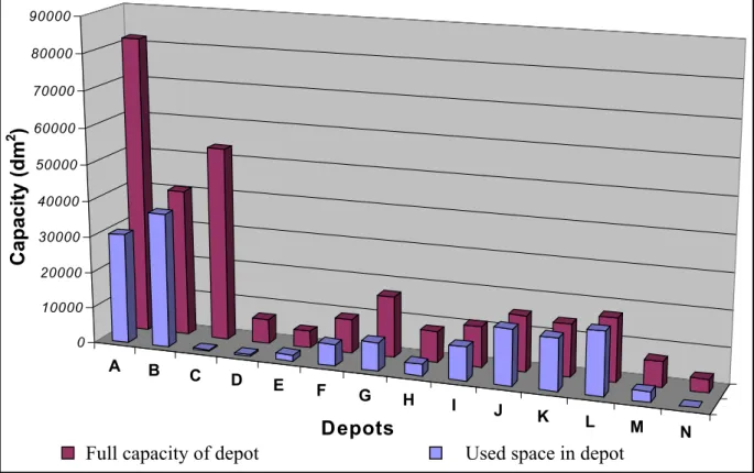
If all the fourteen depots are kept in use for storing, after minimizing distribution and inventory costs, utilization of the depots will be as follow:

Figure 3.1. Utilization of depots with 14 depots.

In depots, which are located in J, K, L, are used at their maximum capacity. But depots that are located in C, D, N, utilization of depots are very low, therefore there is no need to use these depots. For the allocations of items; items that are lower in weight / covered-surface ratio is located at mostly in main depots (wheels, filters), while items that are bigger in this

A _{B C} D _E F _{G H} I _J K _L M _N S 1 S 2 0 10000 20000 30000 40000 50000 60000 70000 80000 90000 Depots Capacity (dm 2 )

ratio are located near to the demand points except safety level of supply level of those items, which are located at main depots.

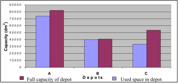
Figure 3.2. Utilization of depots with three depots.

If only main depots want to be used for the inventory of items, depots will have adequate capacity and total utilization will be 83 percent. Again C has the least utilization level among the main depots. A and C will be allocated to items that that are lower in weight / covered-surface ratio (wheels, filters and generators). But the distribution cost is increased as 104 percent. For seeing the relation between number of the depots and distribution costs we run the model for each number of depots and get the following graphic.

Figure 3.3. Restricting the maximum number of depots (M) for the 120-day based stock level.

0 1 0 0 0 0 2 0 0 0 0 3 0 0 0 0 4 0 0 0 0 5 0 0 0 0 6 0 0 0 0 7 0 0 0 0 8 0 0 0 0 9 0 0 0 0 A B C D e p o t s Capacity (dm 2 )

Full capacity of depot Used space in depot

0 2 0 0 0 4 0 0 0 6 0 0 0 8 0 0 0 1 0 0 0 0 1 2 0 0 0 1 4 0 0 0 1 6 0 0 0 1 2 3 4 5 6 7 8 9 1 0 1 1 1 2 N u m b er o f D ep o ts Cost (million TL) 3 4 5 6 7 8 9 1 0 1 1 1 2 1 3 1 4