A PPtlCA TIO N GF GOINTEGRATION ANAl YSIS TO
FHE DEMAND FOR LABOR BY THE TURKISt I
:\TE MANUFAClTJRiNG;SEGTOR. ■
■
■
' A T h m s
SabmitLd to tlie i: paitmentofEconomiC^
and the lr;:b ¡tute o t Lvorior ncs and Sociai Sciences of
Bilkent Univeisity
/
iivPaniaiTiiifiiiment o f the Requii em^ -ts
tor the Oegree of
M A S IE R O F ARTS:ii·: ECONOMICS
Pciuv K A LE cbi iUii y
APPLICATION OF COINTEGRATION ANALYSIS TO
THE DEMAND FOR LABOR BY THE TURKISH
PRIVATE MANUFACTURING SECTOR
A Thesis
Submitted to the Department of Economics and the Institute o f Economics and Social Sciences of
Bilkent University
In Partial Fulfillment of the Requirements for the Degree of
MASTER OF ARTS IN ECONOMICS
by Pelin KALE Febmary 1995
и ъ
Ы О і с
-I certify that -I have read this thesis and in my opinion it is flilly adequate, in scope and in quality, as a thesis for the degree of Master of Arts in Economics.
Assoc. P rof D pfusm an Zaim
I certify that I have read this thesis and in my opinion it is fully adequate, in scope and in quality, as a thesis for the degree of Master of Arts in Economics.
Assoc. P rof Dr. Kıvılcım Metin
I certify that I have read this thesis and in my opinion it is hilly adequate, in scope and in quality, as a thesis for the degree of Master of Arts in Economics.
I
\ a a m / \A ss| c. P rof D ^ Faruk Selçuk
ABSTRACT
APPLICATION OF COINTEGRATION ANALYSIS TO THE DEMAND FOR LABOR BY THE TURKISH PRIVATE MANUFACTURING SECTOR
Pelin KALE MA in Economics
Supervisor: Assoc. Prof. Osman Zaim February 1995
In this study, the demand for labor by the Turkish private manufacturing sector is analyzed for three time periods; 1988 quailer 1-1993 quarter 4, 1988 quarter 1 - 1994 quarter 1, 1988 quarter 1-1994 quarter 2 to be able to capture the effects of the economic crisis of 1994 based on an approach treating employment as a function of output and real wage within an Enor Correction Modeling Approach. In the seaich for possible long run relationships between the vaiiables of interest, Johansen’s Maximum Likelihood procedure is applied to the first difference of variables since all the data series are integrated of order 1. A unique cointegrating relationship is found for each time period. Upon testing and rejecting the exogeneity of the real wage and output series for the demand for labor, short run models are built for each period which are consistent with theoiy but may be subject to biases due to simultaneity between the variables of interest.
Key W ords: Labor Demand, Cointegration, En'or Correction Mechanisms, Turkish Private Manufacturing Sector.
ÖZET
TÜRKİYE ÖZEL İMALAT SANAYİİ SEKTÖRÜNÜN İSTİHDAM TALEBİNİN KOENTEGRASYON TEKNİĞİ KULLANILARAK ANALİZİ
Pelin KALE
Yüksek Lisans Tezi, İktisat Bölümü Tez Danışmanı: Doç. Dr. Osman Zaim
Şubat 1995
Bu çalışmada Türkiye özel imalat sanayii sektörünün istihdam talebi, 1994 yılı ekonomik kıizinin etkilerini de yakalayabilmek amacı ile, üç ayn dönem için (1998, 1.Çeyrek - 1993, 4. Çeyrek; 1998, 1.Çeyrek - 1994, 1. Çeyrek ve 1988,
1.Çeyrek - 1994, 2. Çeyrek) reel ücret ve üretime bağlı bir fonksiyon olarak "EiTor Correction Modeling" (ECM) yaklaşımı ile incelenmiştir. Değişkenlerin durağanlığı birinci gecikmeleri kullamlaıak fark filtresinden geçirilmeleri ile sağlanmış ve uzun dönem ikişkilerinin belirlenmesinde "Johansen's Maximum Likelihood" yöntemi kullanılmıştır. Her dönem için yalnızca bir koentegre ilişki ("Cointegrating Relationship") saptanması üzerine reel ücret ve üretim serilerinin istihdam talebi denklemi için dışsallığı ("weak exogeneity") test edilmiş ve dışsallık varsayımı reddedilmiştir. İncelenen üç dönem için de teori ile tutarlı fakat değişkenlerin eş-anlı belirlenmesinden kaynaklanan hataları da muhtemel olarak içeren, dengesizlik durumlannı yakalamak üzere uzun dönem koentegre ilişkilerden elde edilen ve literatürde "eiTor conection mechanisms" olaıak adlandırılan terimleri de kapsayan kısa dönem istihdam talep denklemleri tahmin edilmiştir.
Anahtar Kelimeler: Koentegıasyon, İstihdam Talebi, Türkiye Özel İmalat Sanayi, Hata Düzeltme Mekanizmalan.
ACKNOWLEDGEMENTS
I am grateful to Associate Prof. Dr. Osman Zaim for his supei-vision and guidance throughout the development of this thesis and would like to thank Associate Prof. Dr. Faruk Selçuk and Associate Prof Dr. Kıvılcım Metin for their valuable comments and suggestions which contributed to the improvements of this study.
I finally and especially would like to thank my family for their encouragements.
CONTENTS
1. Introduction 1
2. Demand For Labor 3
2.1. Demand for Labor in the Short Run 3 2.1.1. Demand by the Firms 3 2.1.2. Demand by the Industry and Market 4 2.2. Demand for Labor in the Long Run 4 2.2.1. Two Factor Case 5 2.2.2. Several Factors 8 2.2.3. Homogenous Labor - Estimation and Empirical Issues 11
2.2.3.1. Estimation 11 2.2.3.2. Measurement and Inteipretation 12 2.2.3.3. Results and Problems 13 2.2.3.3.1. Constant Output and Exogenous Wages 13 2.2.3.3.2. Varying Output or Endogenous Wages 16 2.2.4. Heterogeneous Labor 17
2.2.4.1. Estimation 17 2.2.4.2. Measurement and Interpretation 17 2.2.4.3. Results and Problems 18 2.3. Cointegration in the Analysis of the Labor Market 22 3. A Preview of Cointegration 24
3.1. Cointegration in Econometric Analysis 24 3.2. Main Features of the Theory and Practice of Cointegration Analysis 25 4. Application of Cointegration Analysis to the Demand for Labor by
the Turkish Manufacturing Sector 37
4.1. Data 37
4.2. Analysis of the Short and Long Run Behavior of The Demand for Labor
by the Turkish Private Manufacturing Sector 38 A. Testing for Cointegration Under the Assumption of Nondeterministic
Trends in the Variables 41 i) Testing Through the Maximal Eigenvalue Test Statistic 41 ii) Testing Through the Trace Test Statistic 42 B. Testing for Cointegration Under Assumption of Lineai’ Deteiministic
Trends in Variables and the Data Generation Process 42 i) Testing Through the Maximal Eigenvalue Test Statistic 43
ii) Testing Through the Trace Test Statistic C. The Short Run Models
43 44 5. Conclusion 47 1
1
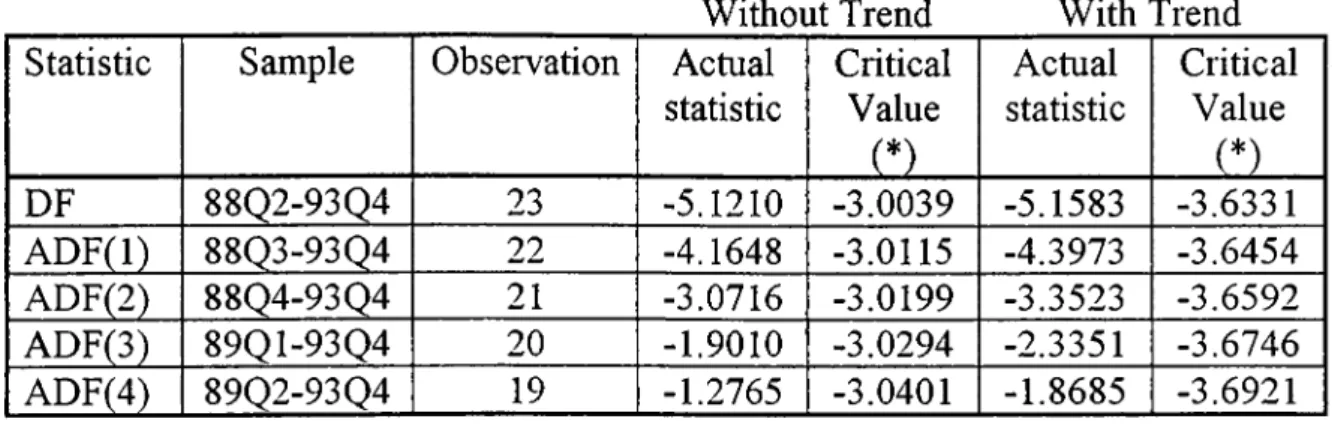
? APPENDICESAPPENDIX A (1988 QUARTER I - 1993 QUARTER 3) I. Unit Root Tests
Table 1 (Unit Root Test for the logarithm of real wage index) Table 2 (Unit Root Test for the logarithm of employment index) Table 3 (Unit Root Test for the logarithm of output index)
Table 4 (Unit Root Test for the first difference of the logarithm of employment index)
Table 5 (Unit Root Test for the first difference of the logarithm of output index)
Table 6 (Unit Root Test for the first difference of the logarithm of real wage index)
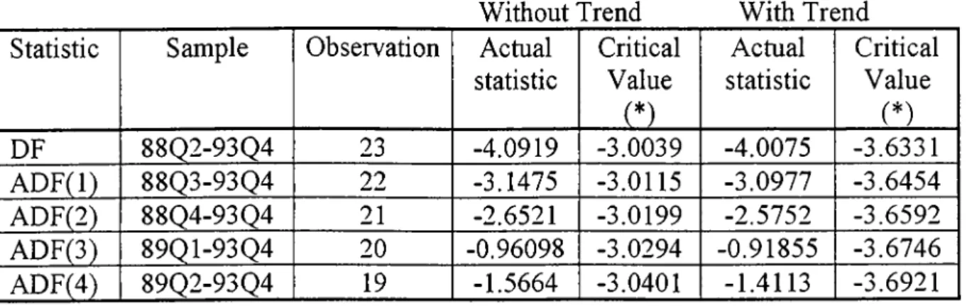
II. Johansen's Maximum Likelihood Procedure (Non Trended Case)
Table 7 (Table for the Determination of Number of Cointegrating Vectors based on the Maximal Eigenvalue Test) 4 Table 8 (Table for the Deteimination of Number of Cointegrating Vectors based
on the Trace Test) 4
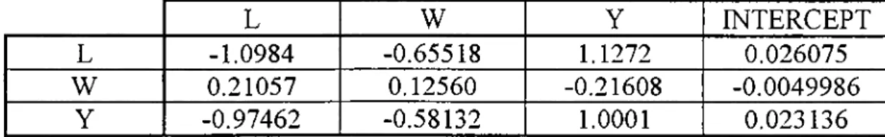
Table 9 (Estimated Cointegrated Vectors) 4 Table 10 (Estimated Adjustment Matiix) 5 Table 11 (Estimated Long Run Matrix) 5 III. Johansen's Maximum Likelihood Procedure (Trended Case, with tiend in Data
Generating Process) 5
Table 12 (Table for the Determination of Number of Cointegrating Vectors based on the Maximal Eigenvalue Test) 6 Table 13 (Table for the Determination of Number of Cointegrating Vectors based
on the Trace Test) 6
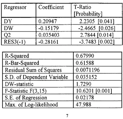
Table 14 (Estimated Cointegrated Vectors) 6 Table 15 (Estimated Adjustment Vectors) 7 Table 16 (Estimated Long Run Matrix) 7 Table 17 (Selected Model) 7 Table 18 (Diagnostic Tests) 8
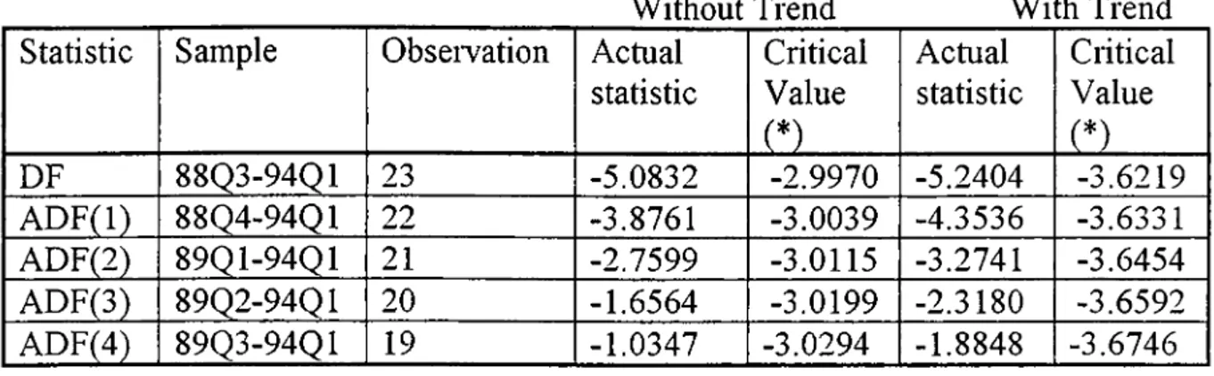
APPENDIX B (1988 QUARTER 1 - 1994 QUARTER 1) I. Unit Root Tests
Table 1 (Unit Root Test for the Table 2 (Unit Root Test for the Table 3 (Unit Root Test for the Table 4 (Unit Root Test for the
employment index)
Table 5 (Unit Root Test for the output index)
Table 6 (Unit Root Test for the of real wage index)
logarithm of real wage index) logarithm of employment index) logarithm of output index)
first difference of the logarithm of first difference of the logarithm of first difference of the logarithm
1
7
1
II. Johansen's Maximum Likelihood Procedure (Non Trended Case) 3 Table 7 (Table for the Determination of Number of Cointegrating Vectors based on the Maximal Eigenvalue Test) 4 Table 8 (Table for the Determination of Number of Cointegrating Vectors based
on the Trace Test) 4
Table 9 (Estimated Cointegrated Vectors) 4 Table 10 (Estimated Adjustment Matrix) 5 Table 11 (Estimated Long Run Matrix) 5 III. Johansen's Maximum Likelihood Procedure (Trended Case, with trend in Data
Generating Process) 5
Table 12 (Table for the Deteimination of Number of Cointegrating Vectors based on the Maximal Eigenvalue Test) 5 Table 13 (Table for the Determination of Number of Cointegrating Vectors based
on the Trace Test) 6
Table 14 (Estimated Cointegrated Vectors) 6 Table 15 (Estimated Adjustment Vectors) 6 Table 16 (Estimated Long Run Matrix) 7 Table 17 (Selected Model) 7 Table 18 (Diagnostic Tests) 7 APPENDIX C (1988 QUARTER 1 - 1994 QUARTER 2)
I. Unit Root Tests
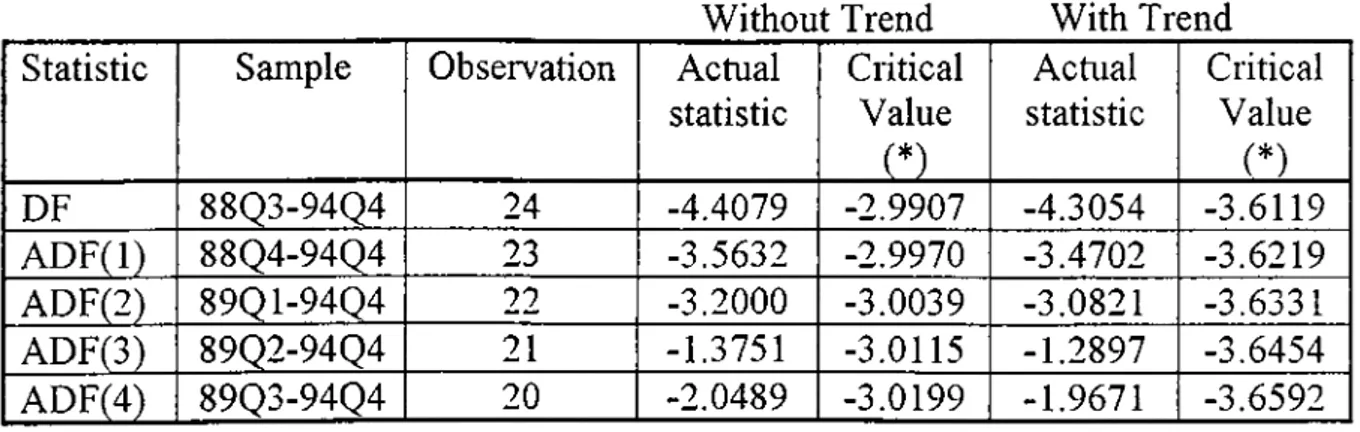
Table 1 (Unit Root Test for the logarithm of real wage index) Table 2 (Unit Root Test for the logarithm of employment index) Table 3 (Unit Root Test for the logarithm of output index)
1
1
7APPENDIX B (1988 QUARTER 1 - 1994 QUARTER 1) I. Unit Root Tests
Table 1 (Unit Root Test for the Table 2 (Unit Root Test for the Table 3 (Unit Root Test for the Table 4 (Unit Root Test for the
employment index)
Table 5 (Unit Root Test for the output index)
Table 6 (Unit Root Test for the of real wage index)
logarithm of real wage index) logarithm of employment index) logarithm of output index)
first difference of the logarithm of first difference of the logarithm of first difference of the logai ithm
1
?
II. Johansen's Maximum Likelihood Procedure (Non Trended Case) 3 Table 7 (Table for the Determination of Number of Cointegrating Vectors based on the Maximal Eigenvalue Test) 4 Table 8 (Table for the Determination of Number of Cointegrating Vectors based
on the Trace Test) 4
Table 9 (Estimated Cointegrated Vectors) 4 Table 10 (Estimated Adjustment Matiix) 5 Table 11 (Estimated Long Run Matrix) 5 III. Johansen's Maximum Likelihood Procedure (Trended Case, with tiend in Data
Generating Process) 5
Table 12 (Table for the Determination of Number of Cointegrating Vectors based on the Maximal Eigenvalue Test) 5 Table 13 (Table for the Determination of Number of Cointegrating Vectors based
on the Trace Test) 6
Table 14 (Estimated Cointegrated Vectors) 6 Table 15 (Estimated Adjustment Vectors) 6 Table 16 (Estimated Long Run Matrix) 7 Table 17 (Selected Model) 7 Table 18 (Diagnostic Tests) 7 APPENDIX C (1988 QUARTER 1 - 1994 QUARTER 2)
I. Unit Root Tests
Table 1 (Unit Root Test for the logarithm of real wage index) Table 2 (Unit Root Test for the logarithm of employment index) Table 3 (Unit Root Test for the logarithm of output index)
1 1 0
Table 4 (Unit Root Test for the first difference of the logarithm of
employment index) 2
Table 5 (Unit Root Test for the first difference of the logarithm of
output index) 2
Table 6 (Unit Root Test for the first difference of the logarithm
of real wage index) 3
II. Johansen's Maximum Likelihood Procedure (Non Trended Case) 3 Table 7 (Table for the Determination of Number of Cointegrating Vectors based on the Maximal Eigenvalue Test) 4 Table 8 (Table for the Deteimination of Number of Cointegrating Vectors based
on the Trace Test) 4
Table 9 (Estimated Cointegrated Vectors) 4 Table 10 (Estimated Adjustment Matrix) 5 Table 11 (Estimated Long Run Matrix) 5 III. Johansen's Maximum Likelihood Procedure (Trended Case, with tr end in Data
Generating Process) 5
Table 12 (Table for the Determination of Number of Cointegrating Vectors based on the Maximal Eigenvalue Test) 5 Table 13 (Table for the Determination of Number of Cointegr ating Vectors based
on the Trace Test) 6
Table 14 (Estimated Cointegrated Vectors) 6 Table 15 (Estimated Adjustment Vectors) 7 Table 16 (Estimated Long Run Matr ix) 7 Table 17 (Selected Model) 7 Table 18 (Diagnostic Tests) 7
APPENDIX D
Testing for Serial Correlation Functional Form Test
Testing for Normality
Testing for Heteroskedasticity Table 19 (Data Used)
1
1 2 9
g r a p h i c s
Graphic 1 (Plot of the logarithm of employment index) Graphic 2 (Plot of the logarithm of real wage index) Graphic 3 (Plot of the logarithm of output)
Graphic 5 (Plot of the logarithm of real wage and employment indexes)
Graphic 6 (Plot of the logarithm of real wage, employment and output indexes) Graphic 7 (Plot of the first difference of the logarithm of employment index) Graphic 8 (Plot of the first difference of the logarithm of real wage index) Graphic 9 (Plot of the first difference of the logarithm of output)
CHAPTER 1
INTRODUCTION
Improved understanding of influences on the demand for labor and its elasticity would contribute to many current labor market concerns such as real wage effects on both the long and the short nm level of employment -which is the main focus of this study-, welfare implications, employment consequence of minimum wages and investment tax credits.
In this study, analysis of the demand for labor by the Turkish private manufacturing industiy based on an approach treating employment as a function of output and real wages will be carried out within an Error Correction Modeling approach. In the search for possible long mn relationships between the variables of interest, a simultaneous equation method for multivariate analysis, namely Johansen's Maximum Likelihood procedure is followed
Chapter 2 is a review of the literature on the demand for labor introducing the fomial theory of labor demand for both the short and the long run with and interest in the elasticity of labor demand. Demand for labor in the long run is examined separately for the two and the multi factor cases (labor demand functions derived from technologies employing two or multi factors). Empirical work carried out on the subject considers the specification of labor demand equations and their estimation methods differentiating between homogeneous and heterogeneous labor; including both the results and problems of estimation, measurement and inteipretation. Finally, application of cointegration techniques to the labor market analysis is discussed in the last section.
Chapter 3 is a preview of an important and relatively recent approach to econometric application: cointegration. Importance and usage of cointegration in econometric time series analysis, closely related literatures, and main features of the theory and practice are discussed, a stepwise analysis of the technique with explanations to useful arguments like the concept of and tests for stationaiity and order of integration of time series. Two main procedures widely used for testing the existence of cointegration; namely the Engle & Granger Two Step Procedure and Johansen’s Maximum Likelihood Estimator are summarised with a special emphasis on the latter which will be utilised in chapter 4 in the deteimination of the cointegrating relationship.
Chapter 4 is the application of cointegration analysis in a general EiTor Collection Modeling approach to the demand for labor by the Turkish private manufacturing sector. In this chapter, the analysis is proceeded for three time periods separately : 1988 quaiter 1-1993 quarter 4, 1988 quarter 1-1994 quarter 1, 1988 quarter 1-1994 quarter 2 in order not to miss the effects of the economic crisis that became severe in 1994. Both a long run relationship between the employment of production workers, real wages and output will be searched and short run models for each period will be built.
The last chapter is devoted to conclusion, where a summaiy of the work perfonned and concluding remaiks aie given.
CHAPTER 2
DEMAND FOR LABOR
The first section of this chapter is a discussion of the formal theory of the demand for labor in the short run. The short run in our discussion is a period in which the only variable factor is labor; whereas the long run will a period in which all factors of production can be varied.
The second section is related to the long run demand for labor, distinguishing between the two and multi factor cases (labor demand functions derived from technologies using two or multi factors) where main focus will be on the elasticity of labor demand. Parameters of interest; the cross-price elasticity and substitution elasticities will be produced for both the two and the multi factor cases and the discussion will be preceded by differentiating between homogenous and heterogeneous labor in reviewing the related empirical work. Several methods for estimation of labor demand equations, results and problems are considered.
Finally, in the third section, applications of cointegration analysis to the labor market will be introduced.
2.1. DEM AND FOR LABOR IN THE SHORT RUN
2.1.1 Demand by the Firms;
The demand for labor in general is a derived demand from the demand for the final product for which it seiwes as a factor of production. The demand for labor by films depends on some factors: technical nature of the production processes (reflected in the production function), revenue from the sales of the output and the input prices.
Let Q = F{L^,K^) be the production function of film / representing the relationship between its inputs and output
where
Qi: Output of film i , L .: Labor input of fiim / ,
:Capital input of firm i .
A profit maximizing fiim will set the marginal value product (price of the output multiplied by the marginal product of the factor) of each input to its marginal cost.
i.e.;
pdF IdL. ,
The rate at which one input can be substituted for another is reflected in the slope of the isoquants, refeixed to as the marginal rate of technical substitution (MRTS). It shows the rate at which labor must be substituted for capital to hold the level of output constant.
MRTS =-dK !L
d U Q
There is also a measure of ease with which labor can be substituted for capital which is the elasticity of substitution. It measures the relative responsiveness of the capital/Iabor ratio to given proportional changes in the MRTS and is given by;
s - d [ K I L ) l { K I L )
d{MRTS)l MRTS
2.1.2. Demand bv the Industry and Market:
The industiy labor demand cuiwe is found by aggregating the demands of all the fimis in the industiy and the market demand is found by aggregating across all industiies in the economy. But the shift of emphasis from the Turn to the industry level or to the market has one consequence: even if the product market is purely competitive, the assumption that changes in output will have no effect on prices is no more valid. Each industiy, different from the finns, faces a downward sloping demand curve. Therefore, if all firms in the industiy employ more labor and increase production, it will result in a fall in product price.
2.2. DEM AND FOR LABOR IN THE LONG RUN
As the supply of labor is not perfectly elastic in the long run; the demand for labor interacts with the shape of the supply function to determine the level of wages.
The interest for the demand for labor might be due to for its own sake or for its effect on wage determination. In some cases like in unionized employment or when the supply of labor is perfectly elastic, the wage can be thought of as being unaffected by labor demand and the knowledge of wage elasticities of labor demand allows to understand the effects of exogenous changes in wage rates on the amount of labor demanded by employers. The effects of changes in the price of one type of labor on its own employment and on that of other types can be discovered by estimation of labor-demand relations alone.
Alternatively, if the employment of workers of a particular type is assumed to be fixed (completely inelastic supply of workers), the demand for labor deteimines the wage rate.
The study of the demand for labor also gives light to policy questions: the effects of any policy that changes factor prices will depend on the structure of the labor demand. The impact of wage subsidies, payroll tax changes, investment credits, etc. can be predicted by estimates of labor demand.
Reminding that the purpose of studying the demand for labor is to understand how exogenous changes will effect the employment and/or wage rates of workers, the main focus will be on the
relations between exogenous wage changes and the deteiinination of employment and on only the static theory of labor demand. The dynamics of labor demand and the role of adjustment costs are ignored.
The examination of labor demand in the long run will be proceeded in two parts: the two factor case and the multi-factor case, without treating the flnn and industiy/market behavior separately.
2,2.1. Two Factor Case;
Many of the specific forms for the production and cost functions were initially developed for the two-factor case where the factors are labor and capital.
Let Y = F{K,L) be a constant returns to scale production function with:
f] > 0; F, < 0; . > 0.
where K and L are homogeneous capital and labor inputs and Y is the output.
A profit maximizing firm will set the marginal value product of each factor equal to its price. Thus:
F,-A = 0
Fi^-Ar = 0where w and r are exogenous prices of inputs and X, is a Lagrangean multiplier and the price of output is assumed as unity.
In the two factor linear homogeneous case, the elasticity of substitution defined previously is:
d{\nK/L) _F,F,
a-d\n(wlr) YF,
The own wage elasticity of labor demand at a constant output and constant r is:
, (1)
where
wL
s = -y- is the share of labor in total revenue.
The cross elasticity of demand (for capital services) is:
Both ( 1) and (2) reflect only substitution along an isoquant (i.e. output is treated as constant). However, when the wage rate increases, the cost of producing a given output rises, and the price of the product will rise, reducing the quantity of output sold. This is the scale effect which depends on the (absolute value) of the elasticity of the product demand, 77 and on the share of labor in total costs. When the scale effects are added;
1 ¡¡ = - {\- s )a -S T] (1’)
(2')
In an individual firm or particular industry which can expand or contract as the wage rate changes, scale effects on employment are relevant. For an entire economy for which the output can be considered at the level of full employment, (T) and (2') are the long run effect of changes in the wage on factor demand.
All of these measures assume that both factors are supplied inelastically to the finn and all the elasticities derived above can be achieved from the alternative approach of cost minimization. Shephard Duality Theorem states that technology may equivalently be represented by a production function or a cost function satisfying certain regularity conditions. Thus there are two ways of obtaining solutions to the derived demand functions, one method is to find a functional foim of the production function and then use Lagrangean or programming techniques in order to obtain the derived demand functions. Alternatively, a functional foiin for the cost function can be postulated and derived demand functions can be estimated by partially differentiating the cost function with respect to input prices. The converse question of what happens to the factor prices in response to an exogenous change in factor supply can be analysed through the use of the elasticity of complementarity; defined as the percentage responsiveness of relative factor prices to a 1 percent change in factor inputs;
c = d\n{wl r)
d\n{KILY
which is just the inverse of the definition of s .
To summarize, in the two factor case with a lineaily homogeneous production technology, elasticities of substitution and complementarity can be found out from either of the production or cost functions.
Some examples of specific production and cost functions are; Cobb-Douglas Technology
The production function is;
Y =
d Y l d L = a Y I L dY! d K = { \ - a ) Y I K
(3) (4)
Since the ratio of (3) to (4) is w/r under profit maximization, taking the logarithms and differentiating with respect to ln(vt^//·) yields cr = 1, and since cr is 1, rj,, - - a) and
% = l - a
Constant Elasticity of Substitution (CHS) Technology The linear homogeneous production function is
where a and p are parameters. The marginal products are:
^ 1 0.= a{YI lT ' ’ (5)
= (6)
Setting the ratio of (5) to (6) equal to w/r, taking logarithms and differentiating with respect to ln(w/r) yields:
o-=l/(l-;9)
Among the special cases of the CES function are: (a) Cobb-Douglas function (p = 0)
(b) the linear function (p = 1) (c) the Leontief function (p = oo).
The CES cost function can be derived as:
C = Y
and the demand for labor is:
L = dC ! dw = a V ‘^Y
Two other functional forms, the generalized Leontief form of Diewert and the ti anslog fonn are second order approximations to arbitraiy cost or production functions. They have the advantage over CES in the two factor case that a is not restricted to be constant but depends on the values of inputs or prices. Their cost functions are examined below.
Generalized Leontief The cost function is:
C = r{a,,w + +¿^22''} 0 )
where ai e pai ameters.
Applying Shephard's lemma for each input, we get:
L a,,+ a,2(w /r)-1/2
K a22+a,2(vr/r)1/2
In general, - depends on all three parameters and the ratio w/r. If a,, = 0, (7) becomes
d[n\w!r)
a Leontief function. If a,, =a^2’ becomes a Cobb-Douglas type function.
Translog
The cost function is:
lnC = InT + a. +a ,lnvr + 0.5/)i(lnvr)“ +6, Invrlnr+ 0.5/>3(lnr)“ +(l-£)! ,)lnr Applying Shephard's lemma to each input and taking the ratios, we get
L · - ^ - +/>| Xnw+KXrir
Again a depends on all parameters and w/r. When , = 0 for all i, the cost function reduces to a Cobb-Douglas Technology. The generalized Leontief and translog functions are useful for empirical work as they allow flexibility and contain simpler forms as special cases.
2.2.2. Several Factors
The theory of demand for several factors of production is just a generalization of the theoiy for the demand for two factors handled in previous parts.
Let F = / (a,, A,,...,^·^) , fj > 0 , fjj < 0 be the production function of a firm (industry, market
or economy). Then the associated cost function based on the demands for A,, A ,,· · ·, is: ^ = where , are input prices. As in the two factor case, the profit maximization requires :
and using the cost function,
where
// and X are Lagrangean multipliers, / == and g.
-Allen (1938) defined <j^ as the partial elasticity of substitution, the percentage effect of a change in , /w . on X J X ^ holding output and other input prices constant as:
f F . . . O', .
-“ X,X,itx(F)
where
det(F) is the determinant of , the bordered Hessian detenninant of the 0 /. - A
= f ,
In Inn,
equilibrium conditions and F]j is the cofactor of in F. A simpler alternative definition based on the cost function is:
giSj
If the system is totally differentiated. [F] . ~dX/X~ dY dX^ — chi\ / X J X , _ dw^ / X F,
Holding Y and other constant, dX^/dv.=--- ^7^ , multiplying the numerator and /Idet(F)
denominator by WjX^XjY; we get:
d\nX,
din Wj = Vij = Y a ,j= s jc x ,.;
which is the elasticity of the demand for input i with respect to input j's price. Multi-factor Cobb-Douelas and CES Functions
The N factor Cobb-Douglas cost function can be written as
i i
The N factor CES production function is:
Y =
Mp
=
1-As with the N factor Cobb-Douglas function, the technological parameters are a·^ = l - p for all /·
The Generalized Leontief The cost function is:
a..
» J
The technological parameters can be estimated from: + z = 1, · · · A^.
The partial elasticities of substitution are:
O’,. = ■Ax,x,h>:j] 0.5 ? and a·,, = 2Z..5,. Translog
In general, the tianslog cost function has the form:
InC = InT +«0 +
with
= 1; by J] by = 0, for all j .
The first and the last equalities are a result of the assumption that C is linear homogeneous in the w.. By Shephard's lemma,
S\n C/ c\n w. - X-wJ C - s., i = \,---,N. s. =a. +j^by\ nwy,
;=i
The partial elasticities of substitution are:
and
- s ) l s ; .
Now, the parameters of interest: the labor-demand, the cross-price and substitution elasticities have been produced for both the two and the multi factor cases. In the preceding part, the specification of the estimating equations and their estimations will be discussed in two main sections, differentiating between homogeneous and heterogeneous labor.
2.2.3. Homogenous Labor -Estimation and Empirical Issues
2.2.3.I. Estimation
Approaches to homogenous labor demand estimation can be summarised as:
Approach 1:
It relies directly on the production or the cost function. In cases of:
a) The Cobb-Douglas function; this method produces the distribution parameters. b) CES function; its estimation is not veiy easy, so direct approach does not apply.
c) The generalized Leontief and Translog functions; they can be estimated directly. In the two factor case, estimation is feasible however, in the multi factor case, there is the problem of multicollinearity.
Approach 2:
It uses labor-demand conditions, either from the marginal productivity condition (derived from profit maximization), or the Shephard condition (derived from cost minimization). In cases of a) A CES function, this means estimating an equation like:
InZ, = «0 + <7\nw ^ +a, Inf .
where a, are parameters with a, = 1 if the production function is characterized by constant returns to scale.
b) A Generalized Leontief and translog functions, since the demand for labor is a nonlinear function of the factor prices, this approach is inconvenient.
In the multi-factor case, this approach involves the estimation of an equation like
\n L= I n w+a, Inf , = 0,
where constant returns to scale can be tested (a, = l). The multi-factor labor demand approach provides a way of testing the homogeneity of degree zero of the demand for labor for factor
prices and of degree 1 in output. A similar approach can be used to examine a wage equation specified as a linear function of the logarithms of all factor quantities.
Approach 3:
It may be called the relative factor demand method. In the two factor CES case this involves the estimation of equation:
a = l / ( l - p ) ^ ~ ^ n ( L/ K)
^ n ( w / r ) ’ (a)
with \n{UK) as a dependent variable, from which demand elasticities can be calculated. This method is invalid for the multi-factor case, as it involves the estimation of all pairs of equations like equation (a) in the CES case or in more general cases, estimation of equations like:
L I K =a ^^{w/rУ'''
a ,2 +a^^_{w/r)''^
\nC = In f+ £JTo +a, lnvr + 0.56,(lnw)' +62lnwln/' + 0.563(lnr)' + (l-a ,)ln / ·.
Approach 4:
It estimates the demand for labor as a part of the system of equations based on one of the approximations, like the generalized Leontief or translog forms.
The methods that have been described above are all related to estimating the constant-output labor-demand elasticity which excludes the scale effects. But, as it has been reminded before, a change in the price of labor will induce a change in output (especially if the unit of obseivation is a small industiy). The effect of which can be measured directly or indirectly. The indirect approach takes some extr aneous estimate of the demand elasticity for the product and uses
<j-sri to derive the labor demand elasticity including the scale effect. A direct
approach estimates equations like those listed below but with output deleted.
In L = + crlnvr +a, Inf
and
InZ, = lnn^. +a, Inf , = 0;
2.2.3.2. Measurement and Interpretation
In this part, concentration is on the measurement of L and w. In the literature , alternatives of the choice of a measure of the quantity L have been total employment and total hours of work. If workers are homogeneous, working the same hours per time period, the choice is iixelevant but if they are heterogeneous along the hours worked per time period, using number of workers will lead to biases if hours per worker are correlated with factor prices or output. In studies
industlies, total hours is more appropriate than employment. In time series data, the choice is not much important, since there is little variation in hours per worker over time. However if dynamics of labor demand is of interest, the choice is crucial since there are significant differences in the rates at which employment and hours adjust to exogenous shocks.
The choice of a measm e of the price of labor is much difficult. Most of the published data from developed countries are on average hourly earnings or average wage rates. A few countries produce data on compensation (employers' payments for fringes and wages per hour on the payroll). While most of the studies use one of the first two measures, none of them is satisfactory. The two problems faced are:
(1) Variations in the measured price of labor may be spurious results of shifts in the distiibution of employment among sub aggregates with different labor costs, or of changes in the amount of hours worked at premium pay.
(2) Data on the cost of adding one worker to the payroll for one hour of actual work are not available.
The second issue is whether to heat some variables as exogenous. Ideally, the labor demand equation will be embedded in an identified model including a labor supply relation. In such a case, methods for estimating a system of equations is appropriate, both the quantity and price of labor might be treated as endogenous.
In studies based on small units, (plants, fiims, small regions) supply cuiwes to those units might be argued to be horizontal in the long mn and thus wage rates might be heated as exogenous. In studies using aggregate data, this assumption has not been considered valid since Malthusion notions of labor supply were abandoned. If the supply of labor to an economy is quite inelastic even in the long run, demand parameters are best estimated using specifications that treat the quantity of labor as exogenous; production functions and variants of second -order approximations including factor quantities as regressors should be used.
In reality, it is unlikely that the labor supply is completely elastic or inelastic, so any choice than estimating production parameters within a complete system that includes supply is unsatisfactoiy. But since supply relations have not been estimated satisfactorily except in some sets of across-section and panel data, one has to make the appropriate choice based on the likely elasticity of supply, the availability and quality of data and about his own interest -whether factor-demand elasticities or elasticities of factor prices are under concern.
_2.2.3.3. Results and Problems
2,2.3.3.1. Constant Output and Exogenous Waees .
The main parameter of interest in studying homogeneous labor is the constant-output own-price elasticity of demand. There are a number of studies that have produced estimates of this parameter. The studies can be divided into two parts: labor demand studies and production or cost function studies which use either a CES production function or a tianslog cost function.
Studies of the constant-output own-price elasticity of demand for homogeneous labor are: I.Labor Demand Studies
A .Marginal productivity condition on labor (estimates of / (1 - i)}
• Black and Kelejian (1970) , covering private nonfarm industiy with quarterly data between 1948-65, with an estimate of 77^ =0.36
• Dhrymes (1969), using private hours and quarterly data between 1948-60, with an estimate of Vll =0.75.
• Drazen et al (1984), using quarterly data of manufacturing hours of 10 OECD countries between 1961-80, with an average of country estimates of = = 0.21
• Hamennesh (1983), using private nonfarm, quarterly data between 1955-78, estimates =as 0.47.
• Liu and Hwa (1974), with private hours and monthly data between 1961-71 estimates = as 0.67.
• Lucas and Rapping (1970), using production hours and annual data between 1930 -65 estimates = as 1.09.
• Rosen and Quandt (1978), with annual private production hours data between 1930-73 estimates = as 0.98.
Studies listed above ai'e based on relationships like InZ =af^ + cr\nw^ +a, InL and since the values of sl are unavailable for the particular samples, estimates of = a are
presented. Estimates here based on a marginal productivity condition imply that the responsiveness of demand is quite consistent with constant-output demand elasticities holding other factor prices constant of between 0.2 and 0.4 (Assuming the share of labor is 2/3 and noticing that the range of most estimates is 0.67-1.09). Only Kelejian and Black and Drazen et al produce estimates that imply a constant-output demand elasticity holding other factor prices constant that is well below this range.
B. Labor demand with price of capital
• Chow and Moore (1972), with quarterly private hours data, from 1948-67 estimates the value of the sample end point 77^^ as 0.37.
• Clark and Freeman (1980), with quarterly manufacturing data from 1950 to 76, when employment stands for labor, estimate as 0.33 and when hours of work stand for labor, estimate it as 0.51.
• Nadiri (1968), with quarterly manufacturing data between 1947 and 64, employment standing for labor, estimate 77^^ as 0.15; and with hours standing for labor, estimate it as 0.19.
• Nickell (1981), using quaiteiiy manufacturing data between 1958-74, estimate 77^^ as 0.19. • Tinsley (1971), using private nonfarm quarterly data between 1954-65, using employment
Studies listed above in part B mostly specify the price of capital semces in a labor demand equation that can be viewed as part of a complete system of demand equations. In these estimates, the own-price elasticity of labor demand is simply the coefficient of Invr^ in the equation containing InZ- as the dependent variable. These estimates are substantially lower that those on pai1 A that include only the wage rate. However the estimates in both parts aie in the same narrow range.
C. Interrelated factor demand
• Coen and Hickman (1970) using annual data of private hours between 1924-40 and 1949-65 estimate as 0.18.
• Nadiri and Rosen (1974), using quarterly manufacturing employment between 1948-65 estimate 77^^ for production as -0.11, and for non-production as 0.14.
• Schott (1978), using aimual British industry data from 1948 to 70 estimate 77^^ as 0.82 with employment standing for labor, and with hours standing for labor, estimate 77^^ as 0.25. Studies of interrelated factor demand by estimating labor and capital demand simultaneously base the labor-demand elasticities in part on the responsiveness of the demand for capital and it is likely that its price is poorly measured. These studies probably don't explain much the demand parameters of interest.
IT. Production and Cost Function Smdies A. CES production function
• Brown and De Cani (1963), using annual private nonfarm hours data from 1933 to 58 estimate 77^^ as 0.47.
• David and Van De Klundert (1965), using annual private hours data between 1899 and 1960 estimate 77^^ as 0.32.
• Me Kinnon (1963), with annual 2 digit SIC manufacturing data, from 1947 to 58, estimate
Vu as 0.29.
B- Translog cost functions
• Bemdt and Khaled (1979), using annual manufacturing data from 1947 to 71, with capital, labor, energy and materials as inputs, assuming homogeneous neutral technology change, estimate 77^ as 0.46 and assuming nonhomothetic, non-neutral technology change, estimate it as 0.17.
• Magnus (1979), with annual enterprise sector data of Netherlands from 1950 to 76, using capital, labor, energy and materials as inputs, estimate 77^^ as 0.3.
• MoiTison and Bemdt (1981) with annual manufacturing data from 1952 to 71, with capital, labor, energy and materials as inputs estimate 77^^ as 0.35.
• Pindyck (1979), with aimual data of 10 OECD countries from 1963 to 73, using capital, labor and energy as inputs estimate 77^^ as 0.43.
Studies listed above in part II produce estimates that are roughly in agreement with those listed in parts I. A and I. B .
In fact, there is no one conect estimate of the constant-output elasticity of demand for homogeneous labor in the aggregate. The hue value of the parameter changes over time as the underlying technology changes, and will differ among economies due to differences in technologies. In developed economies in the late 20^^ centuiy, , the aggregate long run constant-output labor demand elasticity lies roughly in the range 0.15-0.50.
To sum up, an examination of empirical studies indicates that the labor demand elasticity can be obtained from a marginal productivity condition, from a system of factor demand equations, from a labor demand equation that includes other factor prices or from a system of equations that produces estimates of the partial elasticities of substitution among several factors of production.
2.2.3.3.2. Varying Output or Endogenous Wages
The primaiy focus in the long run is the constant-output labor-demand elasticity but, I would like to briefly study what happens to 7 ' in the short run, when the output can vaiy. A shidy by Symons and Layard (1983) examined demand functions for 6 OECD counhies in which only the factor prices, not the output were treated as independent vaiiables . The estimates range from 0.4 to 2.6. These relatively large estimates suggest that there is more room for an imposed rise in real wages to reduce employment when output is let to vaiy.
The discussion about the homogenous labor in the aggregate, and almost all studies summarized treat factor prices including wages as exogenous. To remind, this assumption is valid only if the elasticity of labor supply is infinity which is not implied by studies on data from entire economies. The remarkable similarities of the results discussed in this section may only arise from the use of similar methods which are in fact incoiTect failing to provide a proper test of the theory of labor demand.
Studies that have treated less aggregated data are listed below:
• Ashenfelter and Ehrenberg (1975), using state and local government activities of states , from 1958 to 69 estimate (weighted average of estimates, using employment weights) as 0.67.
• Field and Grebenstein (1980), using annual 2 digit SIC manufacturing data between 1947 and 58 estimate 7^^ as 0.29.
• Freeman (1975)using U.S university faculty data between 1920-70 estimate 77^^ as 0.26. • Hopcroft and Symons (1983) using U.K road haulage data from 1953 to 80, keeping capital
stock constant estimate 7^^ as 0.49.
• Lovell (1973) with 2 digit SIC manufacturing data of 1958 estimate r|^^^ as 0.37.
• Me Kinnon (1963)using annual 2 digit SIC manufacturing data between 1947 and 58 estimate 7j,^ as 0.29.
• Sosin and Fairchild (1984) with 770 Latin American firms between 1970-74 estimate 7^^_ as 0.2
• Waud (1968) with 2 digit quarterly SIC manufacturing data of 1954-64 estimate as 1.03.
The estimates of constant-output labor demand elasticities are quite similar to those summarized above . But even these units of obseiwation are not firms or establishments upon which the theory is based. In contrast to studies of labor supply behavior based on households, there is absence of research on the empirical microeconomics of labor demand. Thus most appropriate tests of the predictions of the theory have yet to be made.
2.2.4. Heterogeneous Labor
2.2.4.I. Estimation;
If it is assumed that there are two types of labor and they are separable from nonlabor inputs, the discussion in the previous section applies. In most cases, the problem is estimating the degree of substitutability among several types of labor and other factors.
Two alternatives are possible, with the choice depending on the availability of data:
(1) A complete system of factor demand equations, a series of N equations with the
L^, i = \...N as the dependent variables and the same set of independent variables as in
In L = ^ b. In w. + ¿7, In Y, ^ = 0
(2) A system of equations based on one of the flexible approximations to the production or cost function (Leontief or translog forms).
Each of these approaches require data on all factor prices and quantities, while the approach using flexible forms allows the ready inference of the partial elasticities of substitution as well as the factor-demand elasticities.
As in the case of homogeneous labor, it is ideal to specify factor demands simultaneously with factor supplies. But if it is difficult to specify such a model involving homogeneous labor, it is impossible to do so for a model including several types of workers. One must be able to argue that supplies of each type of labor are either completely inelastic or completely elastic in response to exogenous changes in demand. No satisfactoiy choice seems to have been made in the studies that have estimated substitution among several types of labor.
2.2.4.2. Measurement and Interpretation
In empirical work estimating substitution among heterogeneous workers, separability in production of labor subaggregates from capital or other groups within the labor force is veiy important.
In separability of labor from capital, in many cases, there is no measure of the price or quantity of capital services. Even if such data are available, they contain large enors of measurement and it may well be argued that hying to aggregate the capital stock in an economy or even in a labor market is senseless. When substitution relations among labor subgroups in the absence of a measur e of capital price or quantity are being estimated, it must be sure that labor is separable from capital. Otherwise, the estimates of labor-labor substitution will be biased.
A similar problem arises for the case of substitution among several subgroups in the labor force when it is assumed that they are separable from the rest of labor (For example, Welch and Cunningham examine substitution among three groups of young workers disaggregated by age under the assumption that the Oy Of each for adult workers are identical). The estimates of the
Oy between the pairs of labor subgroups being studied will generally be biased. The separability should be tested rather than imposed.
Another consideration is the choice of a disaggregation of the work force. Much of the early empirical work focused on the distinction between production and non-production workers This was due partly to the ready availability of data and partly to the belief that such a distinction represented a comparison of skilled and unskilled labor. Recent work suggested that differences in skill between production and nonproduction workers are not so great. Most recent work has disaggregated the work force by age, race, ethnicity, sex, or a combination of these criteria.
The problem of deciding which aggregation to use and the concept of "skill" have led to the definition of some characteristics of workers, according to Welch and Rosen each worker embodies a set of characteristics, letting the data tell what the appropriate skill categories are. 2.2.4.3. Results and Problems:
A summary of the parameters of interest in the studies examining heterogeneous labor disaggregated by occupation is:
Studies of Substitution Among Production and Non Production Workers
Study Data and Method I. Capital Excluded
crbk cw k abw r|bb tiww
A. Cost functions
Freeman and Medoff Manufacturing plants, 1968, 1970 and 1972, detailed
industry dummy variables; CES Union
Nonunion
0.19 0.28
Study Data and Method abk CTwk abw Tjbb T |W W B. Production Functions
Brendt and Christensen Manufacturing, 1929-68; 4.9 -1.63 2.87 Translog, 1968 elasticities
Dougherty States, Census of Population,
1960; CES 4.1
Il.Capital Included A.Cost Functions
Bemdt and White Manufacturing, 1947-71;
Translog, 1971 elasticities 0.91 1.09 3.7 -1.23 0.72 Clark and Freeman Manufacturing, 1950-76
translog, mean elasticities
2.1 -1.98 0.91 -0.58 0.22 Dennis and Smith 2-digit manufacturing
1952-73; translog, mean elasticities.
0.14 0.38 -0.05 Denny and Fuss Manufacturing, 1929-68;
translog, 1968 elasticities
1.5 -0.91 2.06 Freeman and MedoffPooled state and 2-digit
manufacturing industries,
1972, translog. Union 0.94 0.53 -0.02 -0.24 0.12 Nonunion 0.9 1.02 0.76 -0.43 0.61 Grant SMAs, Census of Popul.
1970; translog.
Professionals and managers Sales and clericals
0.47 0.08 0.52 0.32 0.18 Kesselman et al. Manufacturing, 1962-71;
tianslog, 1971 elasticities 1.28 -0.48 0.49 -0.34 0.19 Woodbuiy Manufacturing, 1929-71; translog, 1971 elasticities -0.70 0.52 B. Production Functions
Bemdt and ChiistensenManufacturing, 1929-68; translog
1968 elasticities. 2.92 -1.94 5.51 - 2.1 2.59 Chiswick States, Census of Population,
Study
Denny and Fuss Hansen et al.
Data and Method Professionals vs others. Manufacturing, 1929-68; Translog
1968 elasticities
3 and 4 digit industries, Census of Manufactures,
1967, translog;
highest quartile of plants lowest quaitile of plants
crbk <7wk abw T|bb qww 2.5
2.86 -1.88 4.76
6.0 -1.3 2.0 -1.5
The most consistent finding in the works listed above is: non production workers (presumably skilled labor) aie less easily substitutable for physical capital than are production workers. The own price elasticity is lower the grater is the amount of human capital embodied in the worker. On the issues of the ease of substitution of white for blue collar labor, and about the absolute size of the demand elasticities for each, there is little agreement among studies. However, estimated demand and substnd and substitution elasticities are higher in studies based on p functions.
Only a few studies have disaggregated labor force by educational attainment. Among them. Grant finds that the own price elasticity of demand declines the more education is embodied in the workers.
In more recent studies, a large variety of disaggregations, mostly involving age and/or race and/or sex have been used, which are listed in the table below:
Category
1
Studies of Substitution among Age and Sex Groups
Study Data and Method Types of Labor aij
Elasticities
A. Capital Excluded
Wages Exogenous Welch and States, Census of 14-15,16-17, -Cross Section Cunningham Population, 1970; 18-19 teenage
CES labor -Pooled Cross-sectionGovem. of 17 Australian indust, time series Australia 1976-81; factor
demand equations. M < 2 1 F < 2 1 M > 2 1 + F > 2 1 + all>0 all >0 TjU -1.34 - 1.8 -4.58 -0.59 -2.25
Category Study Data and Method Types of Labor rjil -Time series Johnson and Entire U.S economy, average for 1.43
Blakemore 1970-77; CES 14 age/sex groups
Layard British manufacturing, M < 21 a l l > 0 -1.25 1949-69; F < 18 except -0.31 translog M21+ F<18 -0.35 F 18+ -1.59 B.Capital Included
Wages exogenous Meixilees Canada, Entire, Young males mixed 0.56 -Time series economy 1957-78; Young females -0.44
factor demand Adult Males -0.07 equations. Adult females -0.11 Hamermesh Entire economy. 14-24 all>0 -0.59 1955-75; Translog, 25-44 -0.01 mean elasticities. 45+
Quantities exogenous
-Cross Section Grant SMAs, Census of 16-24 all>0 -9.36 Population, 1970; 25-44 -2.72 Translog. 45+ -2.48 -Time Series Anderson Manufacturing, 1947-72; -7.14
Cross Section Borjas
Translog,
1972 elasticities.
and Factor Prices (Quantities exogenous) A. Capital Excluded
Cross Section Borjas
-3.45 -3.99
Entire U.S economy. Blacks all > 0 -0.77 micro data 1975; Hispanics -0.64 generalized Leontief Whites 0.001
B.Capital Included
Census of Population, Black males 1.02
1970; Females 2.9
Generalized Leontief Hispanic all > 0 Nonmigrants but -2.66 Hispanic not females Migrants andhispan 11.98 White nonmigr. -0.03
Category Study Data and Method Types of Labor cij eu Time-series Grant and Hamermesh Grossman Freeman SMSAs, census of population 1970, tianslog. SMSAs, census of population 1970; translog Entire US economy, 1950-74; translog, mean elasticities. Youths Blacks 25+ White M 25+ White F 25+ Natives Second generation Foreign bom M 20-34 M 35-64 F all>0 -0.03 but -0.43 youth -0.13 vsfema.0.19 all < 0 -0.2 -0.03 -0.23 only -0.38 M20-340.49 vs F is -0.71 >0.
Among above studies, the estimates of factor-demand elasticities vary greatly. However, the demand elasticity for adult men is generally lower than for other groups of workers.
As it was noted before, the elasticity of supply should guide the choice of whether to tieat wages of quantities as exogenous. In the case of disaggregation by age and sex, treating quantities as exogenous and deriving elasticities of complementarity and factor price is a better- choice if data on large geographical units are used. If data on a small industry or firm are used, wages should be treated as exogenous. The studies presented in part II treat quantities as exogenous and estimate these elasticities for a variety of disaggregations of the labor force and give a better indication of the substitution possibilities within the labor force disaggregated by age, race and sex than do those listed in part I.
In all the studies, the elasticities of factor prices are fairly low suggesting that the labor market can accommodate an exogenous change in relative labor supply without much change in relative wages.
Among the studies discussed in this section, only a few has tested the separability of labor from capital. Ber-ndt and Christensen and Dermy and Fuss examine this issue using the production, non-production worker disaggregation. Grant and Hameimesh disaggregate the labor force by age, race and sex. All these studies conclude that separability of labor from capital is not supported by data. They suggest that inclusion of the quantity or price of capital is necessaiy to derive unbiased estimates of production and cost parameters even between subgroups in the labor force. The extent of the biases induced by assuming separability has not been examined. 2.3. COINTEGRATION IN THE ANALYSIS OF THE LABOR MARKET
Existence of long run relationships consistent with theory is very important in the analysis of the labor market Brechlin (1965) and Ball & St. Cyr (1966) examining the relationship between output and employment industries and short term employment functions in British
manufacturing industiies consider the long mn implications of their models. For UK labor markets (aggregate), Andrewes (1986) derives long mn relationships and compares them across different models. Despite this interest, there has not been much work which uses cointegration analysis.
Jenkinson (1986) uses the first stage of the Engle & Granger (1987) two step procedure to determine the existence of a neoclassical long mn relationship between employment, capital stock and real wages. He concludes the OLS residuals are nonstationaiy and rejects the existence of a cointegiating relationship. Ilmakunnas (1989) estimates an enor coixection mechanism for employment which has a single long mn relationship (unique cointegrating vector) between employment, output and real wages for Finnish manufacturing industiy.
However, these articles assume a single cointegrating vector between the variables rather than examining the existence of multiple cointegiating vectors. Alogoskaufis and Smith (1991) examine real wage equations using the Johansen procedure (1988) which allows for multiple long mn relationships among wages, productivity, unemployment and hours of work and finds thiee cointegrating vectors.
CHAPTER 3
A PREVIEW OF COINTEGRATION
The first part of this chapter is an introduction to an important and relatively recent approach to econometric application: cointegration, while the second part covers a detailed analysis of the theory and practice of cointegration analysis.
3.1. COINTEGRATION IN ECONOMETRIC ANALYSIS
Although the non stationary nature of many economic time series has been well known for a long time: Jevons (1884) notes the need 'to avoid any variation due to the time of the year' and also to eliminate 'non periodic variations' in his study of commercial fluctuations, Hooker(1901) discusses the problems of applying the correlation theory 'where the element of time is involved' and argues for analyzing 'the deviations from the trend', the first formal study is by Yule (1926) who examined the conelation between two umelated series such that:
(a) the series were white noise
(b) their first differences were white noise (c) their second differences were white noise
CoiTelation theoiy worked well in case (a) with a nearly noimal conelation distiibution while in case (b), it resembled a semi- ellipse with excess frequency at both ends and in case (c), it was U-shaped so that the most likely coiTelations for the umelated series were ±1.
For the discrimination of spurious from real relationships, it was not until the 1960s when the methods of time series analysis began to influence econometric modeling. Though the time series techniques described by Box and Jenkins (1970) and Granger and Newbold (1977) included both multivariate and univariate techniques, the univariate methods had the most impact. Granger and Newbold (1974) noted the low values of the Durbin - Watson statistic associated with spurious regressions. Phillips (1985), with a formal analysis developed an asymptotic theoiy for regressions between general integrated random processes demonstiating that the distiibutions of the conventional statistics were not the same as those derived under stationarity. The primaiy problem which aiises from attempting to analyse integiated series is that the usual statistical properties of first and second sample moments do not hold. Thus a different distiibution theory is needed. Specifically, the regression coefficients do not converge in probability as the sample size increases: the distribution of the constant diverges and both the regression coefficient and R~ have non-degenerate distributions. The distributions of t-tests also diverge so that there ai'e no asymptotically correct critical values for significance tests.
A closely related literature with cointegration analysis is concerned with the debate: "time series versus econometrics" which states that by analyzing only the differences of economic time series, all information on long run relationships between the levels of economic variables is lost. Sargan(1964) had considered a class of models, later to be known as enor coiTection mechanisms (ECM) which retained levels information in a non integrated form. Granger and
Weiss(1983) introduced the concept of cointegrated series for vaiiables which are individually 1(1) (first difference stationary) but where some linear combination of them is 1(0) (level stationaiy) and Granger and Engle proved that cointegrated series have an ECM representation and conversely, ECMs generate cointegrated series. Later on Stock (1984) proved that if variables are cointegrated, then resulting estimates are super consistent.
Another related literature is concerned with the statistical properties and tests of time series data with unit roots (as 1(1) processes must have) The mathematical-statistical literature on serial conelation includes Anderson (1942), Anderson (1948), White (1958), Fuller (1976), Dickey and Fuller (1979), Hasza and Fuller (1979), Evans and Savin (1981), (1984), Sargan and Bhargava (1983), Bhargava (1983), Phillips (1985, 86), Phillips and Durlauf (1985) and Durlauf and Phillips (1986). The main practical results are t-tests for unit roots in autoregressions based on tabulated critical values (Dickey-Fuller), tests based on the Durbin- Watson statistic (Sargan-Bhargava), and a rapidly increasing body of knowledge of the disti ibutions of the estimators and tests when 1(1) series are involved (Philips).
3.2. M AIN FEATURES OF THE THEORY AND PRACTICE OF COINTEGRATION ANALYSIS
To give an intuition about the concept of cointegiation analysis, an equilibrium relationship of the form:
can be useful.
If F, follows an equilibrium path at each instant, then:
Y, - bX, = 0 at eveiy t.
Out of equilibrium, we may write:
where s, may be interpreted as a disequilibrium error. Engle and Granger (1987) point out that for the concept of equilibrium to have a meaning, "disequilibrium enors", £·, should tend to fluctuate around a common mean or show systematic tendency to become smaller over, time. Equivalently, variables in equilibrium relationship should not drift too far apart and an equilibrium relationship between Y and X implies that the series are cointegrated. The reverse is also tme. Furthermore, an important correspondence exists between cointegrating systems and error correction processes: the relationship between a set of cointegrating variables may be expressed by an Error Correction (EC) representation; converse of which is also tme again. This result is the "Granger Representation Theorem" (Granger, 1983).
Some useful aiguments in the cointegration literature and a stepwise discussion of the analysis is given below.
( 1 ) A series Y, is stationary if its mean, variance and autocovariances are independent of time. More formally, a stochastic process Y, is stationary if:
(i) E{Y,) = /u for all t.
(ii) (iii)
E E
Equations (i) and (ii) require the process to have a constant mean and variance while (iii) states that the covariance between any two values of Y from the series (i.e. autocovariances) depends only on the distance apart in time between these two values. The mean, variance, and autocovariances are independent of time.
The quantities defined by (i) to (iii) are true but unknown population measures for which from any given realization of the process, we have the sample versions defined by;
U ^ T ^ r 'Y ^ Y , i=l m = r ± [ Y , - 7 ) ^ t=\ i{r) = r ' Y { Y , - Y ) ( Y , _ , - Y ) , r=l,2,3,... i=r+l
If the sample autocovariances are obtained by dividing through by the sample variance we obtain the sample autocorrelations:
Stationarity of a series can be investigated by visual inspection of the graph of the sample autocoiTelation against r, known as the coirelogram, however correlogram output is not used as a formal test of stationarity in the cointegration literature. Tests for stationarity will be explained in more detail in the following discussion.
(2) A series Y, is integrated of order d if it becomes stationaiy after differencing d times. This is denoted by:
Y,~ 1(d)