Design of a 4D Trajectory Tracking Controller with
Anti-Windup Protection for Fixed-Wing Aircraft
Kemal Çağlar Coşkun Electrical and Electronics Engineering
Department
TOBB University of Economics and Technology
Ankara, Turkey [email protected]
Artun Sel
Electrical and Electronics Engineering Department
TOBB University of Economics and Technology
Ankara, Turkey [email protected]
Prof. Dr. Coşku Kasnakoğlu Electrical and Electronics Engineering
Department
TOBB University of Economics and Technology
Ankara, Turkey [email protected]
Abstract—This work contains the design and test of a control
scheme for a fixed-wing aircraft to track 4-dimensional waypoints. The controller scheme is a multi-loop design that consists of an inner controller synthesized with the h-infinity loop-shaping method and an outer controller synthesized with the PID method. Multiple inner-loop controllers are synthesized in a state-machine configuration as a measure against saturation windup.
Keywords—fixed-wing, motion control, control system synthesis, anti-windup, multi-loop
I. INTRODUCTION
In parallel to the automation trend in the world, more unmanned aerial vehicles (UAV) are used in the aviation industry to an increasing extent. Consequently, the need for 3-dimensional waypoint tracking increases. Furthermore, adding time-of-arrival (ToA) tracking for 4D trajectory tracking (3 spatial and 1 time dimension) is also increasing in importance as the airspace gets more crowded. For example, accurate ToA planning is important for crowded airports and proposed constant speed methods have issues [1]. Additionally, waypoints with specific ToA constraints will become more necessary as intercity UAV applications scale in scope and size, crowding the airspaces inside metropole areas. Another use case for ToA tracking is obstacle avoidance against other moving objects.
Historically, a multi-loop approach is widely used in navigational waypoint tracking. Where the inner-loop is used for attitude control, the outer-loop is used to track the heading and altitude references [2]. In current research regarding 4D tracking, the majority of studies [3] calculate a speed profile to an already existing 3D trajectory [4][5][6][7], whereas in another study, a P controller is employed from the estimated time error to the airspeed [8].
The ℋ∞ loop-shaping method provides a robust controller for the inner-loop which has been shown to handle large variations of aerodynamic parameters up to 30% [10]. The method was also successfully used in our lab as an attitude controller [11] and as part of a 3D trajectory tracking multi-loop controller architecture [12][13].
Throttle saturation and the ensuing windup is a critical issue in aircraft control which can be dealt with through clamping methods for PID controllers [14] or through rate limiters where high performance is not needed [7][9]. Also, the nested saturation method has been used in some works to deal with actuator saturation [15][16].
Observing current practices, a double-loop control strategy was used in this work. The ℋ∞ loop-shaping method was used to create a robust controller for the inner-loop whereas PID controllers were used in the outer loop. ToA references were added to the outer loop for 4D tracking and a state-machine configuration was employed for protection from the windup.
Although robust methods, 4D tracking methods, and anti-windup methods are present in current literature, these methods have not been combined, which is not a trivial task. The first contribution of this work is to show that a PD controller can be successfully used between the ToA error and airspeed references to track ToA references. Another contribution is the state-machine configuration used against windup which can be applied to any MIMO controller and does not suffer from performance limitations as rate limiters do.
The rest of the paper is organized as follows: Section II describes the computational environment, Section III presents the controller design methodology, Section IV presents the design of the anti-windup scheme, Section V discusses the results, Section VI presents the conclusions.
II. THE PROGRAMMING AND SIMULATION ENVIRONMENTS The control process used in this work is the Cessna 172 aircraft. It is selected for demonstration purposes because it is one of the most widely known airplanes in the aviation industry [17] and the aerodynamic parameters are readily available for the computational model that is used.
The programming environment of this study was MATLAB. Also, Simulink in MATLAB was used to run simulations and make analyzations of the aircraft model. The Cessna 172 continuous-time subsystem of the Airlib [18] library is used as the aircraft model in this work, which is based on the “Flight Dynamics and Control toolbox FDC 1.2” [19] toolbox. This toolbox provides tools to imitate the aircraft through theoretical nonlinear aircraft dynamics equations as found in [20] and to stimulate wind conditions. The inputs of the Airlib subsystem include the elevator, aileron and rudder deflections, the externally applied thrust magnitudes and magnitudes of the external wind. The output port consists of all the states of the aircraft.
Although the FDC 1.2 toolbox is quite comprehensive and suitable for many controller synthesis applications, the extent of its accuracy is finite [19] and some limitations require attention. These limitations include the lack of dynamic models for actuators and sensors and the lack of tools to simulate the effects of discretization and computation delays. Also note that the toolbox offers a tool to simulate engines, but this tool was not added to Airlib which simply asks directly for the applied external force.
The tools used in this work were partially supported by the Scientific and Technological Research Council of Turkey (TÜBİTAK) under Grant 116E187 and the first author was funded by TÜBİTAK through the BİDEB scientist sponsorship program.
This generic subsystem represents different aircraft by setting the relevant parameters to their specific values. The parameters for Cessna 172 given in Table I were already given as an example in the library. Specifically, the used parameters were taken from [21], who in turn based these parameters on the dynamic model of the Cessna 172R aircraft, created by Tony Peden for the open-source program FlightGear [22].
Since Airlib does not simulate actuator dynamics, the inputs were externally saturated during the simulation tests. The saturation values for the controller surfaces were taken directly from the Cessna 172 SP model in X-Plane [23] whereas the maximum thrust value was gathered through testing the same model at the trimmed airspeed at 8400 ft with full throttle command. The maximum deflections are given in Table II.
III. CONTROLLER DESIGN
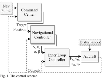
The control scheme consists of two nested control loops and a command center for controlling the simulation. The simplified block diagram is seen in Fig. 1. The controller in the inner loop controls the states of the aircraft that have a relatively high effect on the aerodynamic equations. This controller is termed “the inner loop controller” throughout this paper. The reference states of this controller are the airspeed (𝑉), the pitch angle (𝜃), the bank angle (𝜙), and the sideslip angle (𝛽). The calculated controller outputs are the 4 actuating signals to the propeller system and the control surfaces of the aircraft which are: the total external force along the 𝑋𝑏 axis (the 𝑥 -axis of the body-fixed reference frame) ( 𝐹𝑥), the
elevator deflection (𝛿𝑒), the aileron deflection (𝛿𝑎), and the rudder deflection (𝛿𝑟).
The controller in the outer loop is used to guide states of the aircraft that have either no effect on the flight dynamics or have very little effect. This controller is termed "the navigational controller" throughout this paper. The inputs to this controller are the direction to the next target from the aircraft (𝜓𝑟), the altitude of the next target (𝑧𝑟), and the expected ToA error to the next target. The calculated reference values by the controller are the airspeed (𝑉), the bank angle (𝜙), and pitch angle (𝜃). These outputs are the reference inputs to the inner-loop controller.
The references to the navigational controller are calculated from the 4D position of the target, the 4D position of the aircraft, and the airspeed of the aircraft. This calculation and the incremental selection of targets in a given trajectory are done by a software block termed “the command center” throughout this paper.
A. Inner Loop Controller Synthesis with ℋ∞ Loop-Shaping
Method
For the synthesis of the inner-loop controller, the nonlinear model was first trimmed at a given point and then linearized. The linearized model was then used in the controller synthesis calculations in Section III-A2 to create the ℋ∞ loop-shaping controller.
1) Trim Point and Linearization
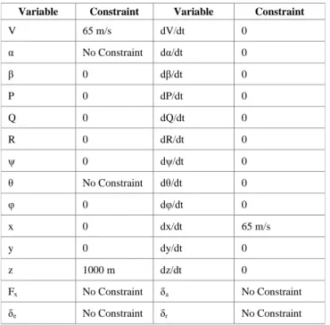
The linearization of the aircraft was made at a stable point with airspeed 65 m/s and altitude 1000 m. The constraints of the trim point calculation are given in Table III. The pitch angle and angle-of-attack angle were not constrained since the altitude derivative was constrained instead.
All constraints were met during the calculation. The trim values of the unconstrained variables are given in Table IV. The trimmed point was verified by observing the nonlinear model through a test simulation without a controller and with the given trim inputs for 10 seconds.
The linearization was done at the trim point with the MATLAB tool linmod.
2) ℋ∞ Loop-Shaping Controller Synthesis
ℋ∞ control design is described as determining the 𝐾(𝑠), the controller so that the ℋ∞ norm of the transfer function from the exogenous input, 𝑤 to the error signals, 𝑧, which are TABLEII. SATURATION VALUES OF CESSNA 172ACTUATORS
Actuator Minimum Maximum
Thrust 0 1300 N Elevator Deflection -28° 24° Aileron Deflection -35° a 35° Rudder Deflection -23.5° b 23.5° a. 20° downwards, 15° upwards b.
Average value of 2 surfaces with maximum amplitudes of 17° and 30°
Fig. 1. The control scheme
TABLEI. CESSNA 172PARAMETERS FOR AIRLIB MODEL
Geometry and Mass
Aerodynamic Derivatives D-Force L-Force 𝑐̅ 1.4935 m 𝑏 10.912 m 𝐶𝐷0 0.031 𝐶𝐿0 0.31 𝑆 16.1651 m2 𝑚 1043.3 kg 𝐶 𝐷𝛼 0.13 𝐶𝐿𝛼 5.143 𝐼𝑥 1285.3 kg·m2 𝐽𝑥𝑦 0 𝐶𝐷𝑞 0 𝐶𝐿𝑞 3.9 𝐼𝑦 1824.9 kg·m2 𝐽𝑥𝑧 0 𝐶𝐷𝛿𝑒 0.06 𝐶𝐿𝛿𝑒 0.43 𝐼𝑧 2666.9 kg·m2 𝐽𝑦𝑧 0 Aerodynamic Y-Moment Derivatives Aerodynamic Y-Force Derivatives Aerodynamic X-Moment Derivatives Aerodynamic Z-Moment Derivatives 𝐶𝑚0 -0.015 𝐶𝑌0 0 𝐶𝑙0 0 𝐶𝑛0 0 𝐶𝑚𝛼 -0.89 𝐶𝑌𝛽 -0.31 𝐶𝑙𝛽 -0.089 𝐶𝑛𝛽 0.065 𝐶𝑚𝑞 -12.4 𝐶𝑌𝑝 -0.037 𝐶𝑙𝑝 -0.47 𝐶𝑛𝑝 -0.03 𝐶𝑚𝛿𝑒 -1.28 𝐶𝑌𝑟 0.21 𝐶𝑙𝑟 0.096 𝐶𝑛𝑟 -0.099 𝐶𝑌𝛿𝑎 0 𝐶𝑙𝛿𝑎 -0.178 𝐶𝑛𝛿𝑎 -0.053 𝐶𝑌𝛿𝑟 0.187 𝐶𝑙𝛿𝑟 0.0147 𝐶𝑛𝛿𝑟 -0.0657
the signals that need to be minimized. This problem is given as
min
𝐾(𝑠)‖𝐹𝑙(𝑃, 𝐾)‖∞ (1) Where 𝑃 is the generalized plant model incorporating the appropriate weight transfer functions so the information about the frequency ranges of disturbance, noise, reference signals are incorporated.
However, by introducing the model uncertainty, which is generally represented in the form of multiplicative input uncertainty, to the problem, the problem complexity arises and turns into a 𝜇 -synthesis problem whose computation is complicated and some numerical stability issues arise and is not preferred for the practical problems where the simple controller is desired.
To account for the model uncertainty, without having to solve a 𝜇 -synthesis problem, ℋ∞ loop-shaping control is suggested by [24], which expresses the family of perturbed plants as, 𝐺𝑝= {(𝑀𝑙+ Δ𝑀𝑙) −1 (𝑁𝑙+ Δ𝑁𝑙) ∶ ‖Δ𝑁𝑙 Δ𝑀𝑙‖∞< 1 𝛾} (2) Which follows from the coprime factorization of the nominal plant 𝐺(𝑠), as
𝐺(𝑠) = 𝑀𝑙−1𝑁𝑙 (3)
Where, the factors satisfy,
𝑀𝑙𝑀𝑙∗+ 𝑁𝑙𝑁𝑙∗= 𝐼 (4) And the problem is expressed as,
min 𝐾(𝑠)𝛾(𝐾(𝑠)) = min𝐾(𝑠)‖[ 𝐾 𝐼] (𝐼 − 𝐺𝐾) −1𝑀 𝑙‖ ∞ (5)
This expression may look as difficult as the mixed sensitivity ℋ∞ control problem, however due to this transformation, the problem simplifies significantly and 𝛾𝑚𝑖𝑛 has an analytical expression,
𝛾𝑚𝑖𝑛= √(1 + 𝜌(𝑋𝑍)) (6) Where 𝜌(∙) indicates spectral radius or maximum eigenvalue as given in [25]. 𝑋 and 𝑍 are the s.p.d. solutions to the two AREs given by,
(𝐴 − 𝐵𝑆−1𝐷𝑇𝐶)𝑍 + 𝑍(𝐴 − 𝐵𝑆−1𝐷𝑇𝐶)𝑇− 𝑍(𝐶𝑇𝑅−1𝐶)𝑍 + 𝐵𝑆−1𝐵𝑇 = 0 (7) (𝐴 − 𝐵𝑆−1𝐷𝑇𝐶)𝑇𝑋 + 𝑋(𝐴 − 𝐵𝑆−1𝐷𝑇𝐶) − 𝑋(𝐵𝑆−1𝐵𝑇)𝑋 + 𝐶𝑇𝑅−1𝐶𝑇 = 0 (8) Where, 𝑅 = 𝐼 + 𝐷𝐷𝑇, 𝑆 = 𝐼 + 𝐷𝑇𝐷 (9) At this point, the controller is given in representative state space from, for a selected 𝛾 > 𝛾𝑚𝑖𝑛 as,
𝐾= [𝐴+𝐵𝐹 + 𝛾2(𝐿𝑇)−1𝑍𝐶𝑇(𝐶 + 𝐷𝐹) 𝛾2(𝐿𝑇)−1𝑍𝐶𝑇
𝐵𝑇𝑋 −𝐷𝑇 ] (10)
Where,
𝐹 = −𝑆−1(𝐷𝑇𝐶 + 𝐵𝑇𝑋) (11) 𝐿 = (1 − 𝛾2)𝐼 + 𝑋𝑍 (12) Since 𝛾𝑚𝑖𝑛 is exactly computable, with an appropriate selection of 𝛾,which agrees with the design specifications, the controller is determined as explained. To incorporate the performance requirements to this problem, instead of using the nominal plant 𝐺(𝑠), 𝐺𝑠(𝑠),
𝐺𝑠(𝑠) = 𝑊2(𝑠)𝐺(𝑠)𝑊1(𝑠) (13) is used, and the controller 𝐾𝑠(𝑠) is found for that shaped plant, where 𝑊1 and 𝑊2 are the filters, used to include the performance specifications 𝑊2 is generally selected as a constant, for our problem 𝑊1 selected to have a closed loop crossover frequency of 3 rad/s.
B. Outer Loop Navigational Tracking with PID Controller
The Navigational Controller scheme is given in Fig. 2. Three PID controllers are used as part of the scheme with values given in Table V. The PID parameters are determined by considering the bandwidth of each loop individually.
The effect of the speed difference on elevator deflections was somewhat too quick in the inner loop. Thus, the action of TABLEIII. CONTSTRAINTS FOR THE TRIM POINT CALCULATION
Variable Constraint Variable Constraint
V 65 m/s dV/dt 0 α No Constraint dα/dt 0 β 0 dβ/dt 0 P 0 dP/dt 0 Q 0 dQ/dt 0 R 0 dR/dt 0 ψ 0 dψ/dt 0 θ No Constraint dθ/dt 0 φ 0 dφ/dt 0 x 0 dx/dt 65 m/s y 0 dy/dt 0 z 1000 m dz/dt 0 Fx No Constraint δa No Constraint δe No Constraint δr No Constraint
Fig. 2. The navigational controller scheme TABLEIV. TRIM RESULTS OF UNCONSTRAINED VARIABLES
Variable Trim Point Variable Trim Point
α -0.0073 rad θ -0.0073 rad
Fx 1126 N δa 0
the time difference to the speed reference was slowed down by negative derivative action.
C. Command Center
The Command Center is a multipurpose software block to aid in simulations during the testing and verification process of this work. It consists of the three blocks seen in Fig. 3. The “Simulation Terminator” stops the test when the last target is reached by the aircraft. This is mathematically determined when the relative position of the target to the aircraft is perpendicular to the aircraft heading.
The position data for the targets are given as a sequential array into the “Target Selector”, which chooses which specific target is the current destination. The 4D position of the targets contains the x and y locations of the targets relative to the initial position of the aircraft as well as their altitude and the required ToAs. The “Target Selector” starts its operation by simply indexing the first target position and then it continues by incrementally selecting the queued targets as the previous targets are reached. The target is updated when the aircraft enters a hypothetical 200 m wide sphere centered at the target. Finally, the “Reference Generator” calculates the orientation of the target relative to the aircraft and reorders the references, adding the reference value 0 as the sideslip angle.
IV. CONTROLLERS FOR THE SATURATED CASE
A. Tracking Error due to Windup
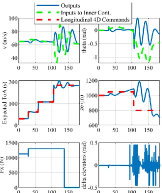
Preliminary results for the design made in Section III are shown in Fig. 4. It is seen from the figure that the aircraft cannot track the altitude reference given. Also, upon further inspection, it is seen that the actuator signal 𝐹𝑥 is behaving unintuitively. This is observed at simulation time 80 when the controller is applying full throttle opposing the expectation that it should reduce the forward thrust since the aircraft is both above its reference altitude and its reference speed. This is due to a phenomenon called windup. From time 30 to 138, the controller is creating an 𝐹𝑥 signal well above the maximum thrust that can be produced and expecting the linear model to act quickly. However, the saturated nonlinear model acts slower, causing a long-lasting error and degenerated controller
states which wind up to a degree where the resulting throttle signal only decreases at time 138 after the wind up is compensated for by a long period of negative error.
The altitude and ToA mismatches are consequences of the inner controller not being able to track the pitch angle and airspeed references. Also, the misbehaving actuator signal 𝐹𝑥 is an output of the inner controller. Thus, it is concluded that the windup problem needs to be solved in the inner controller.
B. Anti-Windup Inner Controller Scheme
In single-input single-output controllers, the states that exhibit the windup phenomenon are easily identified to be between the untracked reference and the misbehaving actuator signal. In such cases, it is possible to easily solve the windup problem by clamping or resetting (via the saturation amount and its derivatives) the states [26] or in cases where performance requirements outweigh simplicity, by various dynamic methods [27].
Methods like the above have also been developed for multi-input multi-output controllers [28]. But if saturation on an actuator is expected to happen many times during normal operation, a specific controller scheme exclusively dealing with this saturated case is preferred to a corrective anti-windup method [29]. Since aircraft dynamics related to ascending, descending, speeding up, and slowing down maneuvers are relatively slow, aggressive use of the throttle actuator is needed for increased performance. Consequently, the throttle signal is expected to saturate regularly, and specific inner controllers are needed for the upper and lower saturated cases of the throttle signal.
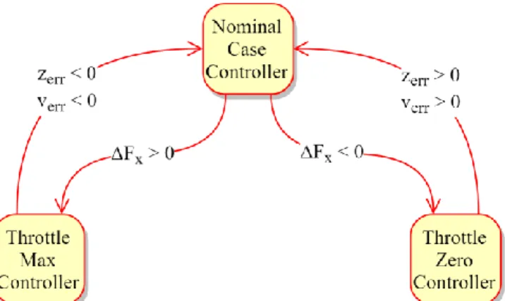
One of these three controllers is selected by a state-machine shown in Fig. 5. The operation starts with the nominal controller selected initially. When Δ𝐹𝑥, the difference between the actuator signal and its saturated value, becomes a positive value, the state switches to the “Throttle Max Controller”, whereas when it becomes a negative value, the “Throttle Zero Controller” is switched on. When the “Throttle Fig. 3. Command center block diagram
Fig. 4. Preliminary results for the controller design without anti-windup TABLE V. PIDPARAMETERS AND SATURATION VALUES
Parameters Saturation P I D Min Max PIDv 0.5 0 -20 - - PIDθ 0.00206 0.0005 0 − 𝜋 2rad - PIDφ 1 0 0 − 𝜋 4rad 𝜋 4rad
Max Controller” gets selected, it stays selected until 𝑧𝑒𝑟𝑟, the altitude reference error, and 𝑣𝑒𝑟𝑟, the airspeed reference error, become negative values, after which, the nominal controller is selected back again. The same switching arrangement is adjusted for the zero-throttle case. It should be noted that the values were not directly compared to zero but to some error margin to prevent infinite switching.
The states of all inner controllers are understandably reset when a switch occurs since the accumulated values of the states will be wrong. Additionally, the PID controller acting between the altitude and pitch angle references (PIDθ) is also
reset during switches, since the pitch angle reference is left untracked while the throttle command is saturated.
C. Specialized Inner Controller Synthesis
The inner controllers for the saturated case are synthesized similar to the nominal case explained in Section III-B. Differently from the nominal case, the controllers for the saturated case can’t control 𝐹𝑥 and thus are left only with the 𝛿𝑒 signal to control the longitudinal dynamics. As a result, these controllers can only control one of the longitudinal references. The airspeed reference is given precedence over the pitch angle reference since the airspeed state is given as a trim constraint and excessive speed losses due to an unexpectedly large pitch angle can cause instability.
The constraints for the trim point calculation are configured to reflect the saturated nature of the thrust. Therefore, the thrust is fixed to its saturated value during the calculation. Also, an aircraft trimmed at a constant airspeed with fixed thrust might climb or descend; thus, the altitude rate was removed as a constraint. Every other aspect of the trim calculation was left the same as in Section III-A1.
The trim points of variables that differ from the ones in Section III-A1 were given in Table VI for the zero-throttle case and in Table VII for the full-throttle case.
The linearization of the aircraft at trim conditions and the synthesis of the controllers were done similarly to how they were done for the nominal case in Section III-A.
V. RESULTS
Simulation results for a test with 4 sample targets are given in Fig. 6, Fig. 7 and Fig. 8. In Fig. 6, the important states of the aircraft are given in solid blue lines. Outermost references related to the targets are given in red dashed lines whereas references created by the command center and fed to the navigational controller are given in purple dashed lines. Finally, the outputs of the navigational controller are given in green dashed lines.
The 3D trajectory of the aircraft and the expected ToA (ToAex) is given in Fig. 7. The 3D locations of the targets are
Fig. 6. Important states of the aircraft and their references during the test simulation Fig. 5. State machine for the inner controller
TABLEVII. TRIM RESULTS FOR FULL-THROTTLE CASE
Variable Trim Point Variable Trim Point
α -0.0073 rad θ 0.0097 rad
Fx 1300 N dz/dt 1.1074 m/s
δe -0.0066 rad
TABLEVI. TRIM RESULTS FOR ZERO-THROTTLE CASE
Variable Trim Point Variable Trim Point
α -0.0077 rad θ -0.1178 rad
Fx 0 N dz/dt -7.1458 m/s
given as green circles and their ToA requirements as dashed red lines. Finally, the actuator signals are given in Fig. 8.
The target positions for this test are given in Table VIII. The xpos, ypos and zpos values represent the 3D location of the
target relative to the initial location of the aircraft in meters. ToA values are relative to the simulation start time and are given in seconds. ToAex is calculated based on the distance
between targets and the average airspeed of the aircraft during the approach to the previous target. Finally, 𝑇𝑜𝐴𝑑𝑖𝑓𝑓= 𝑇𝑜𝐴 − 𝑇𝑜𝐴𝑒𝑥.
Upon inspection of Fig. 6, it is seen that the altitude of the aircraft makes a spike at time 73. This is because a new target with a postponed ToA value was given to the controller. The altitude error due to this maneuver is eliminated with time. There are also frequent oscillations in some states but note that the time scale is quite large, and all references are tracked
successfully. The reference values for the pitch value are missing for some time intervals. One of the saturation controllers is selected during these intervals and a pitch reference is simply not created.
An example simulation is made to compare the system with the anti-windup configuration to the system without it. The targets are given in Table IX, and the results are seen in Fig. 9. The references of the comparison test are given in red dashed lines, the results of the scheme without the anti-windup solution are given in green dotted lines, and finally, the results of the system with the anti-windup configuration are given in solid blue lines. By looking at both the time of arrival and the altitude results, it is seen that the system with the anti-windup compensation tracks the references successfully, whereas the other system becomes unstable.
VI. CONCLUSIONS
The multi-loop controller scheme with an ℋ∞ loop-shaping controller in the inner-loop and some PID controllers in the outer-loop has been shown to track targets with 4D requirements successfully. Also, a state-machine approach with specifically designed controllers has been shown to solve the windup problem of saturated controllers.
TABLEVIII. TARGET POSITIONS OF THE TEST SIMULATION
Target Order xpos ypos zpos ToA ToAex ToAdiff
Target 1 2000 0 1000 30.77 30.77 0
Target 2 4000 2000 1050 74.28 74.28 0
Target 3 6000 2000 1050 115.05 105.05 10
Target 4 9500 -1500 600 195.95 215.95 -20
TABLEIX. TARGET POSITIONS OF THE COMPARISON SIMULATION
Target
Order xpos ypos zpos ToA ToAex ToAdiff
Target 1 2000 0 1000 30.77 30.77 0
Target 2 4000 0 1050 61.54 61.54 0
Target 3 6000 0 1050 112.69 107.64 5
Target 4 12000 0 800 192.95 197.95 -5
Fig. 7. 3D trajectory and ToAex of the aircraft
Fig. 8. Actuator inputs during the test simulation
Future directions related to this work might include adding the orientation of the aircraft at a target as an additional requirement.
REFERENCES
[1] I. A. B. Wilson, "4-Dimensional Trajectories and Automation Connotations and Lessons learned from past research," 2007 Integrated Communications, Navigation and Surveillance Conference, Herndon, VA, 2007
[2] H. Chao, Y. Cao and Y. Chen, “Autopilots for small fixed-wing unmanned air vehicles: A survey,” 2007 International Conference on Mechatronics and Automation, 2007.
[3] R. Dalmau, X. Prats, R. Verhoeven, F. Bussink and B. Heesbeen, “Comparison of Various Guidance Strategies to Achieve Time Constraints in Optimal Descents,” Journal of Guidance, Control, and Dynamics, vol. 42, no. 7, pp. 1612-1621, 2019.
[4] Required time of arrival (RTA) control system, by M. K. DeJonge. (1992, June 9). U.S. Patent 5,121,325 [Online]. Available: https://patents.google.com/patent/US5121325A
[5] Time-responsive flight optimization system, by A. J. M. Chakravarty. (1995, Oct. 10). U.S. Patent 5,457,634 [Online]. Available: https://patents.google.com/patent/US5457634A
[6] Apparatus and method for controlling an optimizing aircraft performance calculator to achieve time-constrained navigation, by J. M. Gonser and R. J. Kominek. (1995, Apr. 18). U.S. Patent 5,408,413 [Online]. Available: https://patents.google.com/patent/US5408413A [7] Aircraft control system for reaching a waypoint at a required time of
arrival, by J. R. Rumbo, M. R. Jackson and B. E. O’laughlin. (2003, Jan. 14). U.S. Patent 6,507,782 [Online]. Available: https://patents.google.com/patent/US6507782B1
[8] R. Dalmau, R. Verhoeven, N. D. Gelder and X. Prats, "Performance comparison between TEMO and a typical FMS in presence of CTA and wind uncertainties", IEEE/AIAA 35th Digital Avionics Systems Conference (DASC), 2016.
[9] Flight management system, by A. P. Palmieri. (1988, Sep. 27). U.S. Patent 4,774,670 [Online]. Available: https://patents.google.com/ patent/US4774670A
[10] C. Kasnakoğlu, “Investigation of Multi-Input Multi-Output Robust Control Methods to Handle Parametric Uncertainties in Autopilot Design,” PLOS ONE, Oct. 2016.
[11] B. Kürkçü and C. Kasnakoğlu, “Robust autopilot design based on a disturbance/uncertainty/coupling estimator,” IEEE Transactions on Control Systems Technology, Aug. 2018.
[12] J. López, R. Dormido, S. Dormido and J. P. Gómez, “A Robust H_∞ Controller for an UAV Flight Control System,” The Scientific World Journal, vol. 2015, 2015.
[13] C. Kasnakoğlu, “Scheduled smooth MIMO robust control of aircraft verified through blade element SIL testing,” Transactions of the
Institute of Measurement and Control, vol. 40, issue 2, pp. 528–541, 2016.
[14] E. Oland and R. Kristiansen, "Adaptive flight control with constrained actuation," 2014 American Control Conference, pp. 3065-3070, June 2014.
[15] R.W. Beard, J. Ferrin and J. Humpherys, "Fixed wing UAV path following in wind with input constraints," IEEE Trans. Contr. Syst. Tech., vol. 22, pp. 2103-2117, Nov. 2014.
[16] S. Zhao, X. Wang, D. Zhang and L. Shen, "Curved path following control for fixed-wing unmanned aerial vehicles with control constraint," J. Intell. Robot. Syst., vol. 89, pp. 107-119, 2017. [17] Textron Aviation, “Cessna Skyhawk.” [Online]. Available:
https://cessna.txtav.com/en/piston/cessna-skyhawk. [Accessed: 20-May-2019].
[18] G. Campa, “Airlib,” File Exchange - MATLAB Central, Mar-2004. [Online]. Available: https://www.mathworks.com/matlabcentral/ fileexchange/3019-airlib. [Accessed: 20-May-2019].
[19] M. O. Rauw, “FDC 1.2—A Simulink toolbox for flight dynamics and control analysis,” Delft Univ. of Technology, Delft, The Netherlands, 1998.
[20] U. Gunes, A. Sel, C. Kasnakoglu and U. Kaynak, "Output Feedback Sliding Mode Control of a Fixed-Wing UAV Under Rudder Loss", AIAA Scitech 2019 Forum, 2019. Available: 10.2514/6.2019-0911. [21] M. S. Selig, R. Deters, and G. Dimock, “Aircraft Dynamics Models for
Use with FlightGear.” [Online]. Available: https://m-selig.ae.illinois. edu/apasim/Aircraft-uiuc.html. [Accessed: 20-May-2019].
[22] FlightGear Flight Simulator. (0.73). FlightGear Project. [23] X-Plane. (10). Laminar Research
[24] Glover, K. and McFarlane, D. (1989) “ Robust stabilization of normalized coprime factor plant descriptions with H_ ∞ bounded uncertainty”, IEEE Transactions on Automatic Control AC-34(8): 821-830
[25] McFarlane, D. and Glover, K. (1990) “Robust Controller Design Using Normalized Coprime Factor Plant Descriptions”, Vol. 138 of Lecture Notes in Control and Information Sciences, Springer-Verlag, Berlin. [26] E. Oland and R. Kristiansen, "Adaptive flight control with constrained
actuation," 2014 American Control Conference, Portland, OR, 2014, pp. 3065-3070.
[27] K. J. Astrom and L. Rundqwist, "Integrator Windup and How to Avoid It," 1989 American Control Conference, Pittsburgh, PA, USA, 1989, pp. 1693-1698.
[28] S. Galeani, S. Tarbouriech, M. Turner and L. Zaccarian, "A Tutorial on Modern Anti-windup Design", European Journal of Control, vol. 15, no. 3-4, pp. 418-440, 2009.
[29] L. Zaccarian and A. R. Teel, Modern anti-windup synthesis: control augmentation for actuator saturation. NJ: Princeton University Press, 2011, p. 3.