1
The renewable energy consumption by sectors and household income growth
in the United States
Andrew A. ALOLA1, a Hakan YILDIRIM 2
Acknowledgement
Author’s gratitude is extended to the editor and anonymous reviewers that will/have spared time to guide toward a successful publication.
1 Department of Economics and Finance, Faculty of Economics, Administrative and Social Science,
Istanbul Gelisim University Turkey.
Corresponding address: [email protected] Mobile: +90 5388 0603701
a
aviola consult ltd, N0. 15 Surulere Street, Kabba, Nigeria. +234 8036982420
2
Istanbul Gelişim University, Faculty of Economics, Administrative and Social Sciences, International Logistics and Transportation, [email protected]
2 Abstract
In the United States, and in most countries, the real Gross Domestic Product grows at a faster pace than the real household income, thus the two indicators could potentially pose dissimilar information. Hence, the study considers the suitability of modelling the United States real disposable personal income (per capita) with the renewable energy consumption across the main sectors: electric and power, industrial and transportation, and residential and commercial. By employing the dynamic Autoregressive Distributed Lag (ARDL) approach, there is a significant and long-run increase in income (real disposable income) growth caused by a per cent increase in the renewables consumed by the industrial sector during the examined period 1973:Q1-2018: Q2. The growth observed in the real growth disposable income with respect to the respective increase in renewable energy consumptions in residential and commercial, electric and power is such that have greater magnitude than the minimum (from the common statistics) income growth. Similarly, the short-run dynamic is significant, like the Granger causality with feedback between income growth and industrial consumption. Granger causality also exists from the real disposable personal income to electric and powers sector consumption of renewable energy with feedback. The study proffers sustainable social and renewable energy mix policies for the United States.
Keyword: renewable energy; real disposable income; household income growth; sector analysis;
3
1. Introduction
Most recently, especially in the advanced nations, the rising concern of climate change has continued to mount pressure on the search for more efficient and alternative sources of energy. Evidently, greater importance has consistently been attached to the traditional sources of energy most especially in advanced nations such as the United States (US) (Alola, 2019a & b). Not until recently when the US government withdrew from the United Nations Framework Convention on Climate Change (UNFCC, 2015) (The Paris agreement), the US Federal policies have subsequently favoured attaining cleaner energy policy. In most of the US states, due to the persistent surge in the growth of renewable energy (RE), the Total Production Energy Source (TPES) from the renewables is expected to be about 12.1% by 2040. Of this volume, electricity generation is projected at about 16% (International Renewable Energy Agency, 2018). Besides, hydropower production suffered a decline of about 2.6% of TPES from 2003 to 2013, energy generation from solar power was observed to double during the same period. During the same period, biofuels and waste were noted to have expanded by about 30.6% of TPES, while 6.2% of TPES was added by geothermal. On a global perspective, the US is the world current leader and highest installer of geothermal energy capacity. Additionally, in 2014, the country accounts for 58 hydroelectric power plants which are capable of powering about 3.5 million homes and generating one billion United States Dollars in revenues. While the country’s goal of doubling the country ’s renewable electricity from wind power, solar power and geothermal resources was attained in 2013 (using the 2008 baseline), the country’s energy policy is now geared at meeting the new target of doubling the same energy source by 2020 using the baseline of 2012.
4
In meeting growing energy demands, active research and developmental collaborations of government agencies like the US Department of Agriculture (USDA), Department of Environment, and Department of Energy (DOE) e.t.c. are tailored toward the cost-effectiveness of the renewable energy source. In spite of the high associated market price of renewable energy compared to the conventional energy sources across most areas of the US, the consumption trend across main sectors has continued to increase. The three-sectoral main components of the renewable energy consumption energy in the US are the electric and power, residential and commercial, and industrial and transportation (EIA, 2018). Consequently, the economy of the country is driven within the three dimensions toward affecting the lives of the end users (consumers), thus information is not available for other sectoral consumption of renewable energy (EIA, 2018). Hence, the market price of RE (as it affects the purpose of consumption per sectors) which is subsequently associated with consumers’ lifestyle (Bin & Dowlatabadi, 2005) is capable of making the US consumers have lifestyle cutbacks across the examined sectors (Dillman, Rosa & Dillman, 1983).
In the light of the above motivation, this study hypothesized a careful examination of the dynamic impacts of the renewable energy consumptions by the electric and power sector, industrial and transportation sector, and the residential and commercial sector on the growth in US real disposable personal income (per capita) in lieu of the gross domestic product (GDP) during the period of 1973:Q1 to 2018:Q2. The study is novel and expectedly contributes significantly to extant literature in few dimensions. Firstly, it shows a paradigm shift from the extant literature that posits that consumers’ lifestyle determines energy or RE consumption (Bin & Dowlatabadi; 2005; Wei, Liu, Fan & Wu, 2007). In this case, the current study considers the reverse case of the above hypothesis. The motive for employing the real disposable income is
5
because the concept of disposable income is a closer idea of income in general economics. This type of income with accounts for taxes and benefits is posed to directly explains the wellbeing of the people and the economy than the national income or the GDP (The Organization for Economic Co-operation and Development, OECD, 2019). Secondly, this study will add to existing literature because it considers sectoral RE consumption rather than considering total RE consumption. It then offers useful empirical information on the market price of sectoral services and the peoples’ (consumers’) lifestyle via the examined RE consumption purposes. Finally, the adopted approach, the Autoregressive Distributed Lag (ARDL) offers a dynamic examination of short-run and long-run relationships.
The rest of the sections are in part. An overview of related studies is presented in section 2. Data and empirical specification are presented in section 3 while the results are discussed in section 4. Section 5 offers concluding remarks that include policy implication of the study and proposal for future study.
2. Energy-income nexus in the US: An overview
The current study deviates from the conventional energy-income (-real GDP or GDP-related) nexus studies in that the (growth in) real disposable income has been employed. However, the prevailing literature have preferred numerous perspectives on energy-income nexus (Appiah, 2018; Bakirtas & Akpolat, 2018; Shahbaz et al., 2018; Alola et al., 2019; Balcilar, Bekun & Uzuner, 2019; Bekun & Agboola, 2019; Borozan, 2019). In some of the earlier studies, especially of a multivariate approach found significant evidence of the relationship between energy and Gross Domestic Product (GDP) (Hamilton, 1983; Masih & Masih, 1996; Stern, 2000; Soytas & Sari, 2003). While significant evidence of energy-GDP cointegration was found in
6
India, Pakistan and Indonesia, no cointegration evidence was found in Malaysia, Singapore and the Philippines (Masih & Masih, 1996). And, for the case of US, Stern (2000) examined the GDP and energy use cointegration for post-war period and found significant evidence of cointegration, thus affirmed that exclusion of cointegration property in the space of discussing is not allowed.
In the United States and similar economies, economic growth has been linked with energy consumption in recent studies (Allen, 1979; Arora & Shi, 2016; Bhattacharya et al., 2016; Aali-Bujari, Venegas-Martínez & Palafox-Roca, 2017; Bekareva, Meltenisova & Guerreiro, 2018). While Bhattacharya et al (2016) investigated the energy-economic growth nexus for top 38 countries, Aali-Bujari, Venegas-Martínez and Palafox-Roca (2017) investigated the relationship by considering the major Organization for Economic Co-operation and Development (OECD) countries. By utilizing a Granger causality and complimented with a Generalized Moment Method (GMM), Aali-Bujari, Venegas-Martínez and Palafox-Roca (2017) found that energy use per capita significantly induced the real GDP per capita in a positive direction in the US and other major economics especially during the period 1977-2014. But, while employing the renewable energy parameter, Bhattacharya et al (2016) found the same positive nexus of energy and economic growth especially in the long-run. However, the specific case of the US was investigated by Bekareva, Meltenisova and Guerreiro (2018) and Arora and Shi (2016). Specifically, Bekareva, Meltenisova and Guerreiro (2018) found a significant and positive short-run impact of energy consumption on the economic growth in Alaska (of the United States) but suggested an indirect impact in the long-run. Interestingly, Arora and Shi (2016) found that total energy-real GDP growth nexus in the US is only bi-directional during the 1990s while it is unidirectional running from the real GDP to total energy consumption in the 2000s. The study
7
also found a similar time-varying relationship between the variables when the different fuel types were employed.
Furthermore, recent studies for the US have also presented the relationship (especially in the long-run) between economic growth (income) and energy consumption across major sectors of the economy (Bowden & Payne, 2009; Kourtzidis, Tzeremes & Tzeremes, 2018). In a multivariate framework, Bowden and Payne (2009) employed the US annual data from 1949 to 2006 to investigate the causal relationship (Toda-Yamamoto long-run causality) between the variables of the subject. The study reveals that the energy-real GDP nexus is not the same across the examined sectors. It implies that while bidirectional Granger-causality exists between commercial and residential primary energy consumption and real GDP respectively, there is Granger-causality from industrial primary energy consumption to real GDP. In addition to examining the country level of energy consumption-economic growth nexus in the US, Kourtzidis, Tzeremes and Tzeremes (2018) examined this aforesaid nexus across the main sectors (Industry, Residential, Electric Power and Transportation) of the country. Unlike the result obtained by Bowden and Payne (2009), Kourtzidis, Tzeremes and Tzeremes (2018) found the neutrality hypothesis of Granger causality tests across all sectors. Moreover, other dimension of the contextual studies have continuously expanded the literature of renewable energy consumption in relation with income in the US and across other countries (Apergis & Payne, 2010; Mozumder, Vasquez & Marathe, 2011; Qiao, Xu, Liu & Chen, 2016; Asonja, Desnica & Radovanovic, 2017; Alola & Alola, 2018).
3. Data and Empirical specification
3.1 Data8
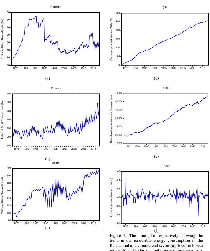
On a general note, the study employed quarterly data spanning from 1973: Q1 to 2018: Q2 after transformation of the series from its initial monthly form. By deploying three-sectoral purpose-driven analysis, we deploy total renewable energy consumed for the purposes of the electric and power sector, industrial and transportation sector, and the residential and commercial sector as the main independent variables. The total renewable energy consumption (TREC) data with restriction to the electric and power, residential and commercial, and the industrial and transportation sectors was retrieved from the US Energy Information Administration (EIA, 2018) are measure in Trillion of British Thermal Units (Btu). Federal Reserve Bank of ST. Louis (FRED, 2018) is the source of a seasonally adjusted (index 1982=100) Consumer price index (CPI) which is employed to accounts for other unobserved factors in the model. Also, the FRED is the source of the dependent variable dataset i.e. the US real disposable personal income per capita3 (seasonally adjusted annual rate). The descriptive statistics as implied in Table 1 and the time plot of the investigated series (see Figure 2) are presented.
<Table 1> <Figure 2> 3.2 Empirical specification
Adopting a subset of the theoretical framework of energy consumption and economic growth adopted in extant literature (Sadorsky, 2012; Al-Mulali & Che Sab, 2018a, b; Rathnayaka, Seneviratna & Long, 2018; Waleed, Akhtar & Pasha, 2018), the current study considers an examination of the dynamic nexus of RE consumption and the disposable income growth. The concern relationship is modelled as:
rdpi t = α + β1lisectort + β2 + β3lrsectort + β3lpsectort + β4lcpit +εt (1)
3 Further information on the US disposable personal income per capita FRED, Federal Reserve Bank of St. Louis;
9
for all t = 1, 2, …, T, rdpi is the growth in the US end users’ real personal income (per capita), βs are the degree of response of the logarithms of the explanatory variables and εis iiid ~ N (μ, σ2). 3.2.1 Dynamic ARDL estimation
We employ the superiority of the Autoregressive Distributed Lag (ARDL) model by Pesaran, Shin and Smith (PSS, 2001) in lieu of other estimation techniques for this investigation. It is effectively applicable for a mixed order of integration which is observed in the results of the unit root estimations (see unit root estimations by Dickey & Fuller, 1979; Kwiatkowski, Phillips, Schmidt & Shin, 1992) shown in lower part of Table 1. In addition to the employed unit root test approaches, we employ the unit root for a single break test by Zivot and Andrews (ZA) (1992) as presented in Table 2. On a second note, the ARDL is considered because it is an effective model for smaller sample sizes. Lastly, specifically for the ARDL-bounds testing approach, it distinguishes between the explanatory and dependent variables. In the estimation procedure, the appropriate maximum lag selection is considered from the common lag length criteria (Akaike Information Criteria –AIC and Schwarz Information Criteria-SIC) for both the dependent and independent variables. Hence, the model deployed is given as:
Δy t = ϕ EC t + ∑ + ∑ + ε t (2)
where ECit = yt-1 – X t θ is the error correction term, ϕ is the adjustment coefficients and β is the long-run coefficients for the period t = 1, 2, … T. Giving the error term εt the dependent variable
yt is the growth in disposable income (rdpit) such that Xt = f (lisector, lpsector, lrsector, lcpi) for
above model (represented as equation 2). The estimation output of the long-run model4 specifications is ARDL(5, 1, 1, 4, 2) and the result is contained in Table 3.
<Insert Table 2>
4 The long-run output is given as: rdpi = 0.001215 – 0.006028*log (rsector) – 0.004438*log (psector) +
10
<Insert Table 3>
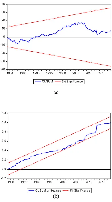
Furthermore, series of diagnostic tests and robustness check that include the Breusch-Godfrey Serial correlation Langrage Multiplier test, Breusch-Pagan-Godfrey Heteroskedasticity test, residual diagnostic (results included in Table 3), and stability tests (see Figure 1) were performed. In addition, the time series Granger causality suggests the direction of impacts (the result is not supplied in the text because of page restriction).
<Figure 1>
4. Empirical results and discussion
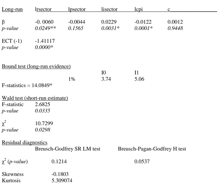
To begin with, the examined series is a mixed order of integration as observed in the results of Dickey and Fuller (1979) and Kwiatkowski, Phillips, Schmidt and Shin (1992) tests (see the lower part of Table 1). Additionally, testing the validity of the single break point observed by Zivot and Andrews (ZA) (1992), there is statistical evidence that the breaks in 2008: Q3 and 2008: Q4 are both significant, especially for specific variables. Indicatively, these periods fall within the global financial crisis which spiralled from the US mortgage market. Thus the period is consequential to the value of the household income in the United States. Proceeding, the results of the ARDL technique employed implies a significant contribution in the context of renewable energy. With a significant quarterly correction of the model (ECT is significant), statistical evidence implies that the US real disposable personal income (rdpi) will respond in the long-run by 0.0060, 0.0044 and 0.023 as the RE consumption increases by 1% in the residential and commercial, electric and power sector and industrial and transportation sector respectively (see Table 3). The observed impacts on the growth of rdpi are significant for the rsector (negatively related) and the isector (positively related), but not statistically significant from the psector. Indeed, declining energy intensity as a result of increased energy efficiency, the
re-11
composition of the energy input, and structural change in the economy are responsible for such observation expressed in the current result (the drifting apart of energy and output) (Stern, 2000). Also, the obvious observation may have been compounded by the specific use of the household income (income per person) as energy consumption as against the conventional GDP per capita commonly employed. However, given that Arora and Shi (2016) and Bekareva, Meltenisova and Guerreiro (2018) respectively found a significant time-variant Granger causality and short-run (only) nexus of energy-economic growth, the findings of the current study are not far-fetched. Also, the rate of increase in cpi will cause a decline in rdpi by 0.012. In corroborating the long-run examination, the bound test rejects the null hypothesis of ‘no long-long-run relationship even at the upper bound i.e 3.74 (I0) ˂ 5.06 (I1) ˂ 14.08 (F-stat.) for the case of using unrestricted intercept and unrestricted trend. Additionally, there is significant statistical evidence of a short-run relationship in the model. Wald test rejects the ‘no short-short-run’ hypothesis with F and chi-square statistics of 2.68 and 10.73 respectively at 5% significant level.
Additionally, the results (renewable energy consumption-disposable income relationship) of the current deviates from the studies that suggests no evidence of long-run relationship between energy and output (income) (Denison, 2011; Solow, 2016; Bekareva, Meltenisova and Guerreiro (2018)). Some of the arguments are based on the fact that energy costs are only a small proportion of GDP, thus energy use is not likely to be a very important factor in changing the rate of economic growth. However, our results affirm the evidence of a positive relationship between changes in capital and energy use per capita especially for a labour-intensive form of production as opined by Moroney (1992). It further clouds the evidence of cointegration opined by Stern (2000). The findings from Stern (2000) suggests that cointegration does occur in the relationship between energy and income in the US, thus energy input cannot be excluded from
12
the cointegration space. Moreover, the result of the current study further affirms the GDP-primary energy consumption per sector nexus presented by Bowden and Payne (2009) but in contrast with the study of Kourtzidis, Tzeremes and Tzeremes (2018).
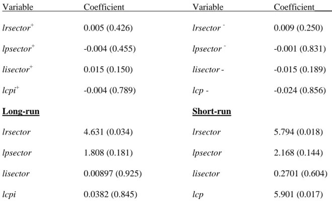
Importantly, statistical evidence indicates that the model does not suffer from regression nightmares that are usually caused by serial correlation and heteroskedasticity as shown chi-square values of Table 3. Also, the residual diagnostic (i.e skewness = -0.18 and kurtosis = 5.4) of Table 3 is desirable. Lastly, using the time series Granger causality test (detail not provided for lack of space), statistical evidence reveals that there is Granger causality from RE consumption by industrial and transportation sector to real disposable personal income with feedback. The same is observed from the real disposable personal income to the electric and power sector but without feedback. Lastly, the model is further investigated as a robustness check by using the asymmetric ARDL (or Nonlinear Autoregressive Distributed Lag, NARDL) and the result is displayed in Table A of the Appendix. From the NARDL result (see Table A), statistical evidence shows that the negative and positive variations of the variables (lrsector, lpsector, lisector, and lcpi) are all not statistically significant. Also, except for lrsector and lcpi, the short-run like the long-run implies that the variables are not statistically significant. Giving that the Ramsey RESET test rejects the null hypothesis of no misspecification (F-stat = 6.333 and p-value = 0.0005), it suggests that the NARDL model is not a better fit (at least for the current investigation), thus affirming the validity of the employed ARDL.
5. Concluding remarks
The study considered renewable energy consumption in the United States three main sectors of electric and power, industrial and transportation, and residential and commercial. It examined the
13
long-run and short-run relationship between renewable energy consumption by the sectors and the United States real disposable personal income (per capita) from the period of 1973Q1 to 2018Q2. Although the impacts from the sector consumption of renewable energy on the growth in the US real disposable personal income is generally small during the examined period, however, it is positive and significant for industrial and transportation, negative and significant for residential and commercial, and positive for electric and power. The negative impact observed is understandable, giving that the minimum value (very low) of the growth in the US real disposable personal income (see descriptive statistics in Table 1) is -0.0415. Hence, our study noted that consumption of renewable energy in the three sectors is significantly responsible for improved growth (although very small) the country’s real disposable personal income. This observed improvement is in the betterment order of residential and commercial sector (given that -0.006 > -0.0415) to electric and power sector (-0.0044 > -0.0415), and to the industrial and transportation sector (0.023 > -0.0415). Visually, the reality aforesaid results are further corroborated in Figure 2. The representation shows a significant decline in the renewable energy consumption in residential (see Figure 2(a)) and the significant increase in commercial sector the renewable energy consumption in residential (Figure 2(c)). In the United States, the huge gap between fossil fuel and alternative energy source consumption for reasons of cost-effectiveness, end-users’ choices, private and government policies, is yet almost stagnant (Mozumder, Vasquez & Marathe, 2011). In spite of the above, the current study showed that renewable energy consumption by the examined sectors of the United States has continued to cause better improvement in the economic lives of the people.
Although the United States government’s policy on the Paris Agreement could potentially signal to bicker especially in the context of attaining cleaner energy through the renewables, other
14
policy instruments could be deployed to advance renewable energy production. To an extent, the states could independently advance policy that advances renewable energy development. For instance, the state of New Mexico Senate Bill 43 mandates investor-owned electric utilities to generate or increasingly purchase amounts of renewable energy (Mozumder, Vasquez & Marathe, 2011). The vast natural resources, vegetation, and the country’s geographical environment are suitable for the production of varieties of renewable energy source. Except for the few like the Eastern New Mexico’s windy landscape, country’s hundreds of thousands of gigawatts (GW) of available land-based resources are yet to be utilized. The central government and the states could further set specific targets for the share of renewable energy source production and take necessary initiative(s) toward its implementation and sustainability. A sustainable renewable energy price subsidy program could encourage more consumption of the energy source across the examined sectors and to the micro-sectors.
The current study has only considered the relationship between energy and sectoral energy consumption at national level, as such this seems to be strong limitation considering the multi-dimensional perspective resulting from the states’ composition of the country. Hence, future study should consider a comprehensive contextual study for the states level for the United States as this would potentially proffer a wider policy outlook. Another limitation is that the current study limits the number of sectors considered to three, as such future study could consider beyond the current three sectors and even across the states. Another econometric approach, such as that examine the frequency and time-varying relationship would further underpin the significance of the research idea.
Funding
15 Compliance with Ethical Standards
The author wishes to disclose here that there are no potential conflicts of interest at any level of this study
Reference
Aali-Bujari, A., Venegas-Martínez, F., & Palafox-Roca, A. O. (2017). Impact of energy consumption on economic growth in major OECD economies (1977-2014): A panel data approach. International Journal of Energy Economics and Policy, 7(2), 18-25.
Allen, E. L. (1979). Energy and economic growth in the United States.
Al-Mulali, U., & Che Sab, C. N. B. 2018a. Electricity consumption, C02 emission, and economic growth in the Middle East. Energy Sources, Part B. Economic, Planning, and Policy, 13(5): 257-263. doi.org/10.1080/15567249.2012.658958.
Al-Mulali, U., & Che Sab, C. N. B. 2018b. The impact of coal consumption and CO2 emission on economic growth. Energy Sources, Part B: Economics, Planning, and Policy, 13(4), 218-223. doi.org/10.1080/15567249.2012.661027.
Alola, A. A., & Alola, U. V. (2018). Agricultural land usage and tourism impact on renewable energy consumption among Coastline Mediterranean Countries. Energy & Environment, 29(8), 1438-1454.
Alola, A. A. (2019a). Carbon emissions and the trilemma of trade policy, migration policy and health care in the US. Carbon Management, 1-10.
Alola, A. A. (2019b). The trilemma of trade, monetary and immigration policies in the United States: Accounting for environmental sustainability. Science of The Total Environment, 658, 260-267.
16
Alola, A. A., Yalçiner, K., Alola, U. V., & Saint Akadiri, S. (2019). The role of renewable energy, immigration and real income in environmental sustainability target. Evidence from Europe largest states. Science of The Total Environment, 674, 307-315.
Apergis, N., & Payne, J. E. 2010. Renewable energy consumption and economic growth: evidence from a panel of OECD countries. Energy policy, 38(1): 656-660. doi.org/10.1016/j.enpol.2009.09.002.
Appiah, M. O. (2018). Investigating the multivariate Granger causality between energy consumption, economic growth and CO2 emissions in Ghana. Energy Policy, 112, 198-208.
Arora, V., & Shi, S. (2016). Energy consumption and economic growth in the United States. Applied Economics, 48(39), 3763-3773.
Asonja, A., Desnica, E., & Radovanovic, L. (2017). Energy efficiency analysis of corn cob used as a fuel. Energy Sources, Part B: Economics, Planning, and Policy, 12(1):1-7. doi.org/10.1080/15567249.2014.881931.
Bakirtas, T., & Akpolat, A. G. (2018). The relationship between energy consumption, urbanization, and economic growth in new emerging-market countries. Energy, 147, 110-121.
Balcilar, M., Bekun, F. V., & Uzuner, G. (2019). Revisiting the economic growth and electricity consumption nexus in Pakistan. Environmental Science and Pollution Research, 26(12), 12158-12170.
Bekareva, S. V., Meltenisova, E. N., & Guerreiro, A. (2018). Arctic Energy Resources as an Economic Growth Factor: Evidence from Alaska, USA. International Journal of Energy Economics and Policy, 8(4), 1-12.
17
Bekun, F. V., & Agboola, M. O. (2019). Electricity consumption and economic growth nexus: evidence from Maki cointegration. Eng Econ, 30(1), 14-23.
Bin, S., & Dowlatabadi, H. 2005. Consumer lifestyle approach to US energy use and the related CO2 emissions. Energy policy, 33(2): 197-208. doi.org/10.1016/S0301-4215 (03)00210-6.
Bhattacharya, M., Paramati, S. R., Ozturk, I., & Bhattacharya, S. (2016). The effect of renewable energy consumption on economic growth: Evidence from top 38 countries. Applied Energy, 162, 733-741.
Bowden, N., & Payne, J. E. (2009). The causal relationship between US energy consumption and real output: a disaggregated analysis. Journal of Policy Modeling, 31(2), 180-188.
Borozan, D. (2019). Unveiling the heterogeneous effect of energy taxes and income on residential energy consumption. Energy policy, 129, 13-22.
Denison, E. (2011). Trends in American economic growth. Brookings Institution Press.
Dickey, D. A., & Fuller, W. A. 1979. Distribution of the estimators for autoregressive time series with a unit root. Journal of the American statistical association, 74(366a):427-431.
Energy International Agency (EIA, 2018).
https://www.eia.gov/energyexplained/index.php?page=about_home.
FRED, 2018. Federal Reserve Bank of St. Louis. https://fred.stlouisfed.org/series/DSPIC96. International Renewable Energy Agency, 2018. Renewable Capacity Statistics 2018. http://www.irena.org/publications/2018/Mar/Renewable-Capacity-Statistics-2018. Hamilton, J. D. (1983). Oil and the macroeconomy since World War II. Journal of political
18
Kourtzidis, S. A., Tzeremes, P., & Tzeremes, N. G. (2018). Re-evaluating the energy consumption-economic growth nexus for the United States: An asymmetric threshold cointegration analysis. Energy, 148, 537-545.
Kwiatkowski, D., Phillips, P. C., Schmidt, P., & Shin, Y. 1992. Testing the null hypothesis of stationarity against the alternative of a unit root: How sure are we that economic time series have a unit root? Journal of Econometrics, 54(1-3): 159-178. doi.org/10.1016/0304-4076 (92)90104-Y.
Masih, A. M., & Masih, R. (1996). Energy consumption, real income and temporal causality: results from a multi-country study based on cointegration and error-correction modelling techniques. Energy economics, 18(3), 165-183.
Moroney, J. R. (1992). Energy, capital and technological change in the United States. Resources and Energy, 14(4), 363-380.
Mozumder, P., Vasquez, W. F.., & Marathe, A. 2011. Consumer’s preference for renewable energy in the Southwest USA. Energy Economics, 33(66): 1119-1126. doi.org/10.1016/j.eneco.2011.08.003.
Pesaran, M. H., Shin, Y., & Smith, R. J. (2001). Bounds testing approaches to the analysis of level relationships. Journal of applied econometrics, 16(3), 289-326.
Qiao, S., Xu, X. L., Liu, C. K., & Chen, H. H. 2016. A panel study on the relationship between biofuels production and sustainable development. International journal of green energy, 13(1): 94-101. doi.org/10.1080/15435075.2014.910784.
Rathnayaka, R. K. T., Seneviratna, D. M. K. N., & Long, W. 2018. The dynamic relationship between energy consumption and economic growth in China. Energy Sources, Part B:
19
Economics, Planning and Policy, 13(5), 264-268.
doi.org/10.1080/15567249.2015.1084402
Sadorsky, P. 2012. Energy consumption, output and trade in South America. Energy Economics, 34(2): 476-488. doi.org/10.1016/j.eneco.2011.12.008.
Shahbaz, M., Zakaria, M., Shahzad, S. J. H., & Mahalik, M. K. (2018). The energy consumption and economic growth nexus in top ten energy-consuming countries: Fresh evidence from using the quantile-on-quantile approach. Energy Economics, 71, 282-301.
Solow, R. M. (2016). Resources and economic growth. The American Economist, 61(1), 52-60. Soytas, U., & Sari, R. (2003). Energy consumption and GDP: causality relationship in G-7
countries and emerging markets. Energy economics, 25(1), 33-37.
Stern, D. I. (2000). A multivariate cointegration analysis of the role of energy in the US macroeconomy. Energy economics, 22(2), 267-283.
The Organization for Economic Co-operation and Development (OECD, 2019) https://data.oecd.org/hha/household-disposable-income.htm. (Retrieved 09 May 2019) UNFCC, C. 2015. Paris agreement. FCCCC/CP/2015/L. 9/Rev.1
Waleed, A., Akhtar, A., & Pasha, A. T. 2018. Oil consumption and economic growth: Evidence from Pakistan. Energy Sources, Part B: Economics Planning, and Policy, 13(2): 103-108. doi.org/10.1080/15567249.2017.1354100.
Wei, Y. M., Liu, L. C., Fan, Y., & Wu, G. 2007. The impact of lifestyle on energy use and C02 emission. An empirical analysis of China’s residents. Energy policy, 35(1): 247-257. doi.org/10.1016/j.enpol.2005.11.020.
20
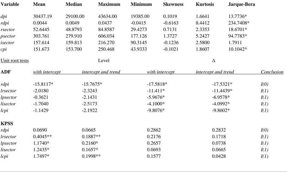
Table 1: Descriptive statistics and Unit root test with ADF and KPSS______________________________________________________________ Variable Mean Median Maximum Minimum Skewness Kurtosis Jarque-Bera
dpi 30437.19 29100.00 43634.00 19385.00 0.1019 1.6641 13.7736* rdpi 0.0044 0.0049 0.0437 -0.0415 -0.6163 8.4412 234.7408* rsector 52.6445 48.8793 84.8587 29.4273 0.7131 2.3353 18.6701 * psector 303.761 279.910 606.034 177.126 1.3727 5.2427 94.7783 * isector 157.614 159.813 216.270 90.3145 -0.1236 2.5800 1.7911 cpi 151.673 153.700 250.468 43.9333 -0.1021 1.8607 10.1042 *
Unit root tests Level Δ
ADF with intercept intercept and trend with intercept intercept and trend Conclusion
rdpi -15.8117* -15.7675* -17.5818* -17.5321* I(0) lrsector -2.0180 -2.3243 -11.411* -11.4439* I(1) lpsector -0.3621 -2.1431 -5.9676* -6.9578* I(1) lisector -1.7040 -2.5173 -4.1000* -4.0992* I(1) lcpi -1.1429 -2.1922 -9.8076* -9.8602* I(1) KPSS rdpi 0.0690 0.0665 0.2862 0.2832 I(0) lrsector 0.4045** 0.1887** 0.2176 0.1718 I(1) lpsector 1.1740* 0.2160* 0.2657 0.0738 I(1) lisector 1.2435* 0.1657* 0.0693 0.0665 I(1) lcpi 1.7497* 0.1998** 0.1577 0.0428 I(1)
Note: Level and Δ respectively indicates estimates at level and first difference with automatic lag selection by SIC (maxlag=13) for the ADF (Augmented Dickey Fueller) and KPSS () unit root test. * and ** are statistical significance at 1% and 5% level. A number of observation is 181. Also, lrsector, lpsector and lisector are the logarithmic of residential and commercial sector, electric and power sector, and industrial and transportation sector respectively.
21
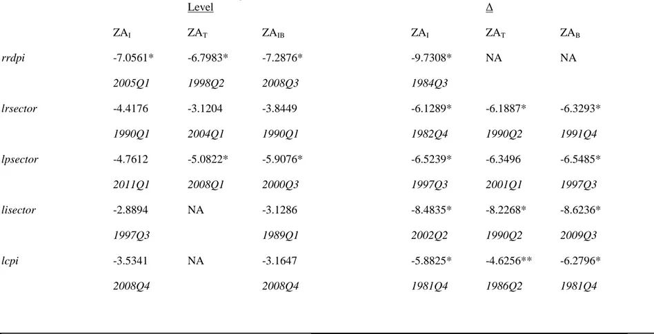
Table 2: Zivot-Andrew (ZA) unit root test under single structural break____________________________________________________________
Level Δ ZAI ZAT ZAIB ZAI ZAT ZAB rrdpi -7.0561* -6.7983* -7.2876* -9.7308* NA NA 2005Q1 1998Q2 2008Q3 1984Q3 lrsector -4.4176 -3.1204 -3.8449 -6.1289* -6.1887* -6.3293* 1990Q1 2004Q1 1990Q1 1982Q4 1990Q2 1991Q4 lpsector -4.7612 -5.0822* -5.9076* -6.5239* -6.3496 -6.5485* 2011Q1 2008Q1 2000Q3 1997Q3 2001Q1 1997Q3 lisector -2.8894 NA -3.1286 -8.4835* -8.2268* -8.6236* 1997Q3 1989Q1 2002Q2 1990Q2 2009Q3 lcpi -3.5341 NA -3.1647 -5.8825* -4.6256** -6.2796* 2008Q4 2008Q4 1981Q4 1986Q2 1981Q4
Note: Level and Δ respectively indicates estimates at the level and first difference. Automatic lag selection by SIC (maxlag=4) for unit root test and maxlag=4 for ZA). ZA is the
Zivot & Andrews (1992) for a unit root structural break test where ZAI, ZAT & ZAB are an intercept, trend and intercept with the trend of ZA estimates. Also, lrsector, lpsector
22
Table 3: Dynamic ARDL estimate__________________________________________________
Long-run lrsector lpsector lisector lcpi c_________________
β -0. 0060 -0.0044 0.0229 -0.0122 0.0012
p-value 0.0249** 0.1565 0.0031* 0.0001* 0.9448 ECT (-1) -1.41117
p-value 0.0000*
Bound test (long-run evidence)
I0 I1
1% 3.74 5.06
F-statistics = 14.0849*
Wald test (short-run estimate) F-statistic 2.6825 p-value 0.0335 χ2 10.7299 p-value 0.0298 Residual diagnostics
Breusch-Godfrey SR LM test Breusch-Pagan-Godfrey H test χ2
(p-value) 0.1214 0.0537
Skewness -0.1803
Kurtosis 5.309074
Note: Autoregressive Distributed Lad (ARDL) model employed is (5, 1, 1, 4, 2), β is the coefficient of the regressors, the p-value is the probability value and ECT is the Error Correction Term also known as the adjustment parameter. The I0 and I1 are lower and upper bound of the bound test respectively (using unrestricted intercept and unrestricted trend case), χ2 is the Chi-square, SR LM is Serial correlation Lagrange Multiplier and H is Heteroskedasticity. And, * and ** are statistical significant values at 1% and 5% significance level respectively. Also, lrsector, lpsector and lisector are the logarithmic of residential and commercial sector, electric and power sector, and industrial and transportation sector respectively.
23 -40 -30 -20 -10 0 10 20 30 40 1980 1985 1990 1995 2000 2005 2010 2015 CUSUM 5% Significance (a) -0.2 0.0 0.2 0.4 0.6 0.8 1.0 1.2 1980 1985 1990 1995 2000 2005 2010 2015
CUSUM of Squares 5% Significance
(b)
24 20 30 40 50 60 70 80 90 1975 1980 1985 1990 1995 2000 2005 2010 2015 Rsector T ri ll io n o f B ri ti s h T h e rm a l U n it s ( B tu ) (a) 100 200 300 400 500 600 700 1975 1980 1985 1990 1995 2000 2005 2010 2015 Psector T ri ll io n o f B ri ti s h T h e rm a l U n it s ( B tu (b) 80 100 120 140 160 180 200 220 1975 1980 1985 1990 1995 2000 2005 2010 2015 Isector T ri ll io n o f B ri ti s h T h e rm a l U n it s ( B tu (c) 40 80 120 160 200 240 280 1975 1980 1985 1990 1995 2000 2005 2010 2015 CPI C o n s u m e r p ri c e i n d e x (i n d e x 1 9 8 2 = 1 0 0 ) (d) 15,000 20,000 25,000 30,000 35,000 40,000 45,000 1975 1980 1985 1990 1995 2000 2005 2010 2015 Rdpi D is p o s b a le i n c o m e p e r c a p it a ( th o u s a n d d o ll a r) (e) -.06 -.04 -.02 .00 .02 .04 .06 1975 1980 1985 1990 1995 2000 2005 2010 2015 RRDPI R e tu rn t o i n c o m e ( th o u s a n d d o ll a rs ) (f)
Figure 2: The time plot respectively showing the trend in the renewable energy consumption in the Residential and commercial sector (a), Electric Power sector (b) and Industrial and transportation sector (c). Also, the time plot (d), (e), and (f) are respectively the consumer price index, the disposable income and the return to disposable income.
25 Appendix
Table A: Dynamic Asymmetric ARDL______________________________________________ Dependent Variable: Δ rrdpi
Variable Coefficient Variable Coefficient_________
lrsector+ 0.005 (0.426) lrsector - 0.009 (0.250) lpsector+ -0.004 (0.455) lpsector - -0.001 (0.831) lisector+ 0.015 (0.150) lisector- -0.015 (0.189) lcpi+ -0.004 (0.789) lcp - -0.024 (0.856) Long-run Short-run lrsector 4.631 (0.034) lrsector 5.794 (0.018) lpsector 1.808 (0.181) lpsector 2.168 (0.144) lisector 0.00897 (0.925) lisector 0.2701 (0.604) lcpi 0.0382 (0.845) lcp 5.901 (0.017)
Cointegration test statistics: t-BDM = -8.0414 (> F-PSS = 7.8593) Diagnostic Test
Portmanteau test: χ2
= 46.02 p-value = 0.2372 Breusch/Pagan Heteroskedasticity test: χ2
= 1.405 p-value = 0.2359 Ramsey RESET test: F-stat = 6.333 p-value = 0.0005*
Jarque-Bera test on Normality: χ2 = 2.74 p-value = 0.2541
Note: χ2 is the Chi-square, p-value is the probability value, t-BDM is the test value for the Banerjee, Dolado and Mestre (BDM, 1986), F-PSS is the F-statistic of the Pesaran, Shin and Smith (PSS, 2001), * indicates statistical significant at 1% significance level. Also, lrsector, lpsector and lisector are the logarithmic of residential and commercial sector, electric and power sector, and industrial and transportation sector respectively.