Learning based cross-coupled control for multi-axis high precision positioning systems

LEARNING BASED CROSS-COUPLED CONTROL FOR MULTI-AXIS HIGH PRECISION

POSITIONING SYSTEMS

Nurcan Gecer Ulu

Mechanical Engineering Department Bilkent University

Ankara, 06800 Turkey

E-mail: ulu@bilkent.edu.tr

Erva Ulu

Mechanical Engineering Department Bilkent University

Ankara, 06800 Turkey

E-mail: erva@bilkent.edu.tr Melih Cakmakci

Mechanical Engineering Department Bilkent University

Ankara, 06800 Turkey

E-mail: melihc@bilkent.edu.tr

ABSTRACT

In this paper, a controller featuring cross-coupled control and iterative learning control schemes is designed and implemented on a modular two-axis positioning system in order to improve both contour and tracking accuracy. Instead of using the standard contour estimation technique proposed with the variable gain cross-coupled control, a computationally efficient contour estimation technique is incorporated with the presented control design. Moreover, implemented contour estimation technique makes the presented control scheme more suitable for arbitrary nonlinear contours. Effectiveness of the control design is verified with simulations and experiments on a two-axis positioning system. Also, simulations demonstrating the performance of the control method on a three-axis positioning system are provided. The resulting controller is shown to achieve nanometer level contouring and tracking performance. Simulation results also show its applicability to three-axis nano-positioning systems.

INTRODUCTION

Increasing demand for micro/nano-technology related equipment resulted in a growing interest for precision positioning. Multi-axis precision positioning is required in micro/nano-scale manufacturing and assembly, optical component alignment systems, scanning microscopy applications, nano-particle placement applications, cell/tissue engineering and etc. [1-3]. Most of the time, these applications require both high contour and tracking accuracy.

In tracking control, the objective is moving along a desired trajectory. Although almost all systems employ feedback as a part of tracking control, substantial improvement of tracking accuracy is achieved by the addition of feed forward control methods. In literature, several feed forward control schemes have been shown to improve tracking accuracy such as zero phase error tracking control (ZPETC) [4-6], feed forward friction compensation [7, 8] and iterative learning control (ILC) [9, 10]. According to Tomizuka [4], tracking performance of a ZPETC system is sensitive to variations in plant parameters and modeling errors since ZPETC design is based on pole/zero cancellation and phase cancellation. Moreover, friction compensation techniques generally incorporate a system identification process that should be repeated if system parameters change. On the other hand, Tan et al. [9] claims that specifying a plant model for ILC via zero phase filtering is not necessary considering the principle of self-support that is argued in [11] because the stored control signals reflect the plant characteristics. In other words, ILC can improve tracking performance of a system even the plant structure and nonlinearities are unknown [12]. Yet, the system should execute the same task repetitively to be able to implement an ILC scheme.

Generally, improving tracking accuracy of each individual axis also increases contouring accuracy of the multi-axis system. However, in some cases, decreasing the tracking error may not decrease the contour error; it may even deteriorate the ASME 2012 5th Annual Dynamic Systems and Control Conference joint with the

JSME 2012 11th Motion and Vibration Conference DSCC2012-MOVIC2012

DSCC2012-MOVIC2012-8660

contouring performance [13]. Hence, control structure should be designed considering not only tracking error but also contour error in order to achieve high accuracy in both. Koren [14] proposed the cross-coupled control (CCC) that focuses on eliminating contour error rather than individual axes errors. This method is proven to reduce contour error significantly. Since the introduction of CCC, it has been modified and combined with different control techniques. Some examples are observer-based CCC [15], cross-coupled model reference adaptive control [16], cross-coupled iterative learning (CCILC) [10], CCC with disturbance observer and ZPETC [6], CCC with friction compensation [8] and CCC with ILC [10, 17].

Since CCC based control schemes require contour error as the control parameter, there is a need for construction of a contour error model in real time. Contour error is defined as distance between actual position and the nearest position on the contour [18]. Although, contour error can be calculated for linear contours, this calculation is very complicated for nonlinear contours, especially during the operation. Hence, some approximations have been used to calculate a nonlinear contour error. Koren [13] suggested circular contour assumption. Then, Yeh and Hsu [18] proposed a method to approximate contour error as the vector from the actual position to the nearest point on the line that passes through the reference position tangentially. As the authors mentioned, although circular contour assumption works well for biaxial motion systems, it is difficult to apply on multi-axis systems.

The work presented aims to provide an improved method for precision motion control featuring CCC and ILC. Although CCC and ILC have been used together in [10] and [17] for contours combining lines and circles, the new method also benefits from the contouring error estimation vector approach. In this way, the new method is computationally more efficient, more suitable for coupling gain calculations of arbitrary nonlinear contour and easier to implement on multi-axis systems. Moreover, for the best of our knowledge, this is the first time CCC and ILC is used together to achieve nanometer level precision and implemented on a three-axis system. SYSTEM SETUP

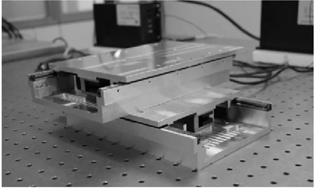
The two-axis positioning system is constructed by assembling two modular single-axis stages perpendicularly as in Fig. 1. A modular single-axis stage is designed with a stationary base and a moving slider that are connected to each other via cross-roller linear bearings. The stage is actuated by a brushless permanent magnet linear (PMLM) motor with 120mm travel range whereas the position feedback is taken from an incremental linear encoder. The linear encoder has an optical scale with four micrometer grating in pitch leading one micrometer resolution. Yet, the encoder resolution is increased to 25 nanometers using an interpolation technique. Details of interpolation procedure can be found in [19].

Idealized dynamic model of a single-axes linear stage is given in Fig. 2 where R is linear motor resistance, L is linear

FIGURE 1. TWO-AXIS MODULAR POSITIONING SYSTEM

motor inductance, KBEMF is back electromotive constant, Kforce is force constant, m is sliding mass, b is viscous friction, e is linear motor input voltage, Kamp is amplifier gain and i is linear motor current. In the dynamic model, ripple forces of the PMLM are neglected and linear bearings are modeled as viscous friction component. From the dynamic model, mathematical model of the linear stage is found as in Eq. (1).





After the system is modeled, a suitable PID feedback controller is obtained using traditional methods.

FIGURE 2. DYNAMIC MODEL OF A SINGLE-AXIS STAGE

CONTROL DESIGN

In this paper, an improved method based on CCC and ILC which benefits from the contouring error vector approach has been presented. Next two subsections will briefly describe ILC scheme used in this work and CCC. Moreover, contour estimation approaches will be explained together with CCC. The last subsection will mention the insight of the improved method.

Iterative Learning Control (ILC) via Zero Phase Filtering

ILC is a technique for improving the transient response of a system that operates repetitively. ILC can often be used to achieve perfect tracking, even when the model is uncertain or unknown and there is no information about the system structure and nonlinearity [12]. ILC based on zero phase filtering is a practical and efficient implementation of ILC [9].

Block diagram of ILC via zero phase filtering for an individual axis is given in Fig. 3. In the diagram, superscript i is iteration number whereas uffi and ufbi are feed forward and feedback control signals at ith _{iteration. The feed forward}

control signal for ith _{iteration is calculated using the feed}

forward and feedback control signals of the previous iteration that are shown as uffi-1 and ufbi-1 respectively. The learning update law can be given as in Eq. (2) [9].

1 1

( )

( )

(

)

2

1

u k

u

k

u

k

j

M













where k is the time index, γ is the learning gain and M is the length index of zero phase filter. Some guidelines for the design of parameters γ and M can be found in [9].

FIGURE 3. BLOCK DIAGRAM OF ILC VIA ZERO PHASE FILTERING WITH FEEDBACK CONTROLLER

Cross-Coupled Control (CCC)

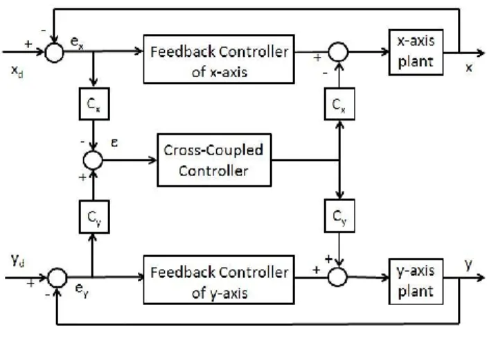
Cross-coupled control is a special type of multi input multi output (MIMO) control which aims to decrease the contour error. Block diagram of this control scheme is given in Fig. 4. In the block diagram, Cx and Cy are coupling gains whereas ε, ex, ey are the contour error, x-axis tracking error and y-axis

tracking error respectively. As can be observed form Fig. 4, contour error is obtained through the equation

x x y y

C e C e

    (3)

Although CCC is first introduced with constant gains in [14], the term CCC is generally used for CCC with variable coupling gains as proposed in [13]. For a nonlinear contour, calculation of these coupling gains is very complicated. Therefore, some contour error approximations are needed to simplify the coupling gain computation. For this purpose, Koren [13] proposed circular contour assumption. Then, Yeh and Hsu [18] presented contour error vector approach. The next two parts will briefly describe these approaches.

Circular Contour Assumption. In this approach any arbitrary contour is separated into parts with radius of curvature ρ and these parts are approximated by circles. Since contour error for a circular contour is the difference between the

FIGURE 4. BLOCK DIAGRAM OF CCC

distance from the actual position to the center of the circle and radius of the circle, contour error for an arbitrary contour can be written as

2 2

0 0

(x x ) (y y )

       (4)

where (x0, y0) and (x, y) denote center of the curvature and actual position, respectively. Expressing the actual position with respect to reference position and axial tracking errors (ex, ey) and using Taylor expansion, approximated contour error becomes (cos ) (sin ) 2 2 y x y x e e e e          (5)

where θ is traversal angle of motion. In Eq. (5), ρ becomes infinity for linear contours.

Contouring Error Vector Approach. Contour error vector approach can be explained through the geometrical relations in the multi-axis motion control system given in Fig. 5. In the figure, 𝑒⃗ is tracking error vector, 𝜀̂⃗ is estimated contour error vector, 𝜀⃗ is contour error vector, 𝑡⃗ is normalized tangential vector, 𝑛⃗⃗⃗⃗ is normalized normal vector, P is actual position and R

is reference position. In this approach, contouring error 𝜀⃗ is defined as the vector from the actual position to the nearest point on the line that passes through the reference position tangentially with direction 𝑡⃗ [18]. This approach estimates contour error vector very closely when tracking error is small enough. Looking at Fig. 5, 𝜀̂⃗ is equal to 〈𝑒⃗ , 𝑛⃗⃗⃗〉 where 〈. , . 〉 is

inner product operator. Hence, relation between 𝜀̂⃗ and 𝑒⃗ can be obtained using inner product. Furthermore, the contour error is calculated as |𝜀̂⃗| =∑𝑖𝐶𝑖𝑒𝑖 (i=x, y, z …) where Ci is coupling gain and ei is the corresponding axial tracking error. Considering these two representations of estimated contour error vector, cross coupling gains (Cx, Cy, Cz …) in terms of normalized

normal vector ( 𝑛⃗⃗⃗⃗ = [nx ny nz …]T )are found as Ci = ni (i=x, y, z,

Although two different approaches give similar results in terms of contouring accuracy, contour error vector method has several advantages over the circular contour assumption. Firstly, it is computationally more efficient. Moreover, with contour error approach, coupling gains can be computed easier for an arbitrary contour. Also, implementation of circular contour approach to a multi-axis system is difficult [18].

FIGURE 5. GEOMETRICAL RELATIONS OF CONTOUR ERROR (ADOPTED FROM [18])

The Improved Method

The presented work is a part of project that aims to design a controller for a three-axis positioning system with nanometer level tracking and contouring performance. The three-axis positioning system is designed such that three modular single-axis stages will be assembled on top of each other to build it. As a logical step to validate our multi axis modular control approach, a two-axis positioning system has been assembled as shown in Fig 1. This paper focuses on real time control of two-axis system; however the feasibility study of three-two-axis positioning system is given to illustrate the expected results in the 3 axis system currently under development. The control system is intended to be modular considering being able to interchange the stages without changing the control system. For

modularity concerns, ILC is chosen for improving tracking performance since controller structure does not change with changes in plant model structure and parameters. Moreover, contouring error vector method chosen to be used with CCC since it is computationally more efficient. As mentioned before, encoders of the positioning system have been interpolated to achieve nanometer resolution. This procedure is accomplished without any extra hardware. Due to this fact, there is a trade of between resolution of the encoders and the computational effort in the control loop. Therefore, it is aimed to minimize computational effort in the control loop to maximize encoder resolution. Using contouring error vector technique also makes the control method more suitable to implement on three-axis systems and to operate with arbitrary nonlinear contours. To sum up, a control method featuring CCC and ILC via zero phase filtering as in Fig. 6 has been developed incorporating the contouring error vector estimation technique.

SIMULATION ANALYSIS

In order to verify the performance the two-axis positioning system, simulation analysis has been provided. Moreover, feasibility study of the control method on three-axis positioning system is conducted. In the simulations, velocity profiling has been used to generate individual-axis reference trajectories. Generic s-curve method is employed for this purpose.

Simulations in Two-axis

Two-axis positioning system has been simulated with a nonlinear contour. In the proposed approach, it is straight forward to find coupling gains when the equation of the curve is known since coupling gains are just elements normal vector elements of the contour. Plant model is simulated with feedback control (FB), feedback control with cross-coupled control (FB&CCC), feedback control with iterative learning control (FB&ILC) and feedback control with cross-coupled

TABLE 1. TWO-AXIS SYSTEM - SIMULATION RMS ERROR VALUES FOR THE NONLINEAR CONTOUR

Control Method RMS Error of X-Axis [nm] RMS Error of Y-Axis [nm] RMS Contour Error [nm] FB 11.30 111.27 39.04 FB & CCC 15.42 110.65 32.36 FB & ILC 3.47 2.17 2.73 FB & CCC & ILC 1.09 2.11 0.78

FIGURE 7. TWO-AXIS SYSTEM SIMULATION - RMS ERROR VALUES FOR THE NONLINEAR CONTOUR

FIGURE 8. SIMULATION OF TWO-AXIS SYSTEM FOR THE NONLINEAR CONTOUR

control and iterative learning control (FB&CCC&ILC). Effects of all simulated control schemes on the performance are summarized in Tab. 1 and Fig. 7. In the table and figure, root mean square (RMS) of the error signals has been used. It can be observed that combining ILC and CCC with FB gives the best results as expected. This combination benefits from both tracking performance improvements of ILC and contouring performance improvements of CCC. For the designed control system, ILC convergence has been achieved around 20 iterations. In other words, there is no significant decrease in the errors after 20 iterations. Hence, FB&ILC and FB&CCC&ILC simulation results are recorded after 20 iterations.

The nonlinear contour used in simulations is given in Fig. 8. In the figure, the zoomed view is taken from the part with a sharp turn that is shown with the box on the original contour because contour tracking is more difficult on sharp turns. As can be seen in zoomed view of Fig.8, contouring performance of the system for the nonlinear contour is improved significantly when the proposed method (FB&CCC&ILC) is used instead of only feedback (FB) control.

Simulations in Three-axis

Simulations and experiments have been conducted on the two-axis system to show the effectiveness of the proposed system. However, in this work, it is also claimed that the proposed method can be easily implemented on a three-axis system. In order to demonstrate it, proposed method is simulated for three axis system. Reference contour is a 45o

inclined circle with 7 micrometers radius as given in Fig. 10. As mentioned previously, coupling gains can be obtained from the normal vector of the contour. Using that approach coupling gains have been found without too much computational effort. In the zoomed view of Fig. 10, it has been observed that the proposed method has very good tracking performance compared with the feedback control. Moreover, reference contour and the resulting contour of the FB&CCC&ILC control is almost coincident. This also confirms the very small RMS tracking errors and RMS contour error observed in Tab. 2.

FIGURE 9. SIMULATION OF THREE-AXIS SYSTEM FOR THE NONLINEAR CONTOUR

Simulation results of three-axis system given in Tab. 2 and Fig. 10. Looking at the results, it is observed that contour error decreases with FB&CCC whereas individual axis errors may deteriorate. Yet, when the ILC is also added to the control scheme both individual and contour errors decrease significantly. For these simulations, combined CCC and ILC gives the best contour and tracking accuracy. Moreover, it can also be observed that FB&ILC control decreases individual axis tracking errors by 63% - 85%- 63%, contour error 46%. When CCC is added to FB&ILC controls contour error decreases 72% and individual tracking errors decrease by %36 – 43% - %63. This observation confirms ILC is especially efficient in tracking control whereas CCC is especially effective for contour control.

0 20 40 60 80 100 120 RMS Error of

x-Axis RMS Error ofy-Axis RMS ContourError

R M S E rr or V alue s [n m ] FB FB & CCC FB & ILC FB & CCC & ILC

Moreover, combining both controllers results in a controller which is effective for both tracking and contouring.

EXPERIMENTAL RESULTS

Velocity profiling with s-curve is used to obtain individual axis trajectories in the experimental results section. For experimental results, the same contour with same velocity profiling designed for simulations part is used. Contour tracking of the two-axis system with only feedback (FB) control and feedback control with CCC and ILC (FB&CCC&ILC) is given in Fig. 11. Looking at the zoomed view, it is obvious that presented control design improved contouring performance considerably. When Fig. 7 and Fig.11 is compared, it should be noted that simulations and experiments give similar behavior such as deteriorated contour control just after the sharp turn. Moreover, FB&CCC&ILC system gives better contouring result than FB. Yet, in experimental results, FB&CCC&ILC design does not improve the contouring performance as much as simulation. This result is reasonable considering unmodeled system dynamics or disturbances.

TABLE 2. THREE-AXIS SYSTEM SIMULATION - RMS ERROR VALUES FOR THE NONLINEAR CONTOUR

Control Method RMS Error of X-Axis [nm] RMS Error of Y-Axis [nm] RMS Error of Z-Axis [nm] RMS Contour Error [nm] FB 235.87 144.26 235.87 86.07 FB & CCC 268.06 177.19 209.68 59.12 FB & ILC 33.07 51.44 33.07 46.29 FB & CCC & ILC 21.22 29.78 12.29 13.55

FIGURE 10. THREE-AXIS SYSTEM SIMULATION - RMS ERROR VALUES FOR THE NONLINEAR CONTOUR

Experiments are conducted on the system with feedback control (FB), feedback control with cross-coupled control (FB&CCC), feedback control with iterative learning control (FB&ILC) and feedback control with cross-coupled control and iterative learning control (FB&CCC&ILC). FB&ILC and FB&CCC&ILC experimental results are recorded after 20

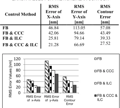
iterations. Variation of RMS single-axis errors and RMS contour error with the different control schemes is given in Fig.12 and Tab.3. Looking at Tab. 3, it can be observed that FB&CCC system decreases contour error significantly whereas changes in axial errors are not as significant. Similarly, FB&ILC system decreases axial tracking errors more effectively than contour error as expected. Best tracking and contouring performance is obtained for FB&CCC&ILC system as for the simulation case. All axial tracking errors and contour error is improved around 50%. This improvement is higher for simulations however this is acceptable since simulations are performed for idealized systems in idealized conditions.

FIGURE 11. EXPERIMENTAL RESULTS OF TWO-AXIS SYSTEM FOR THE NONLINEAR CONTOUR TABLE 3. TWO-AXIS SYSTEM - EXPERIMENTAL RMS

ERROR VALUES FOR THE NONLINEAR CONTOUR

Control Method RMS Error of X-Axis [nm] RMS Error of Y-Axis [nm] RMS Contour Error [nm] FB 46.84 113.05 57.08 FB & CCC 42.06 94.66 43.49 FB & ILC 25.81 79.14 39.33 FB & CCC & ILC 21.28 66.69 27.52

FIGURE12. TWO-AXIS SYSTEM - EXPERIMENTAL RMS ERROR VALUES FOR THE NONLINEAR CONTOUR

0 50 100 150 200 250 300 RMS Error of x-Axis RMS Error of y-Axis RMS Error of z-Axis RMS Contour Error R M S E rr or V alue s [n m ] FB FB & CCC FB & ILC FB & CCC & ILC 0 20 40 60 80 100 120 RMS Error

of x-Axis RMS Errorof y-Axis ContourRMS Error R M S E rr or V alue s [n m ] FB FB & CCC FB & ILC FB & CCC & ILC

CONCLUSION AND FUTURE WORK

In this paper, a new method which is computationally more efficient, more suitable for coupling gain calculations of arbitrary nonlinear contour and easier to implement on multi-axis systems is presented. Tracking and contouring performance of the method on a nonlinear contour is verified through simulations and experiments achieving nanometer level accuracy for the two-axis system. In the experiments, RMS error of x-axis, RMS error of y-axis and RMS contour error of the two-axis system is decreased to 21nm, 66nm and 27nm, respectively. Considering encoder resolution, the smallest value encoder can detect, is 25nm, resultant positioning is very accurate. Having RMS error less than the resolution means that trajectory is followed very closely and error value has been zero in some parts of the motion. Furthermore, a feasibility study of the presented method on three-axis system is conducted and results are promising. In future, real time implementation of the method on three-axis system will be practiced.

ACKNOWLEDGMENTS

This research is sponsored by Scientific and Technical Research Council of Turkey (TUBITAK) through Project No: 110M251. The authors would like to thank undergraduate students Oytun Ugurel and Ersun Sozen for their support during computer aided design and drafting of the positioning system. Authors would also like to thank Dr. Sinan Filiz for sharing his experience in precision positioning systems.

REFERENCES

[1] Manske, E., Hausotte, T., Mastylo, R., Machleidt, T., Franke, K., and Jager, G., 2007. “New Applications of the Nanopositioning and Nanomeasuring Machine by Using Advanced Tactile and Non-tactile Probes”. Measurement Science and Technology, 18(2), pp. 520-527.

[2] Lihua, L., Yingchun, L., Yongfeng, G., and Akira, S., 2010. “Design and Testing of a Nanometer Positioning System”. Journal of Dynamic Systems, Measurement, and Control, 132(2), pp. 02011-6.

[3] Pang, C. K., Guo, G., Chen, B. M., and Lee, T. H., 2006. “Self-sensing Actuation for Nanopositioning and Active-mode Damping in Dual Stage HDDs”. IEEE/ASME Transactions Mechatronics, 11(3), pp. 328-338.

[4] Tomizuka M., 1987. “Zero Phase Error Tracking Algorithm for Digital Control”. J. Dyn. Sys., Meas., Control, 109(1), pp. 65–68.

[5] Hsu, P., Houng, Y., and Yeh, S., 2001. “Design of an Optimal Unknown Input Observer for Load Compensation in Motion Systems”. Asian Journal of Control, 3(3), pp. 204–215.

[6] Qing, L., Tai-yong, W., Jing-chuan, D., Yong-xiang, J., and Bo, L., 2010. “Applications of position controller for CNC machines based on state observer and Cross Coupled Controller”. 2010 International Conference on Computer,

Mechatronics, Control and Electronic Engineering (CMCE), IEEE, pp. 593–596.

[7] Tomizuka, M.,2007. “Friction Compensator for Feed Drive Systems Consisting of Ball Screw and Linear Ball Guide”. Proceedings of the 35th International MATADOR Conference, pp311-314.

[8] Wang, L., Lin, S., and Zheng, H., 2011. “Precision Contour Control of XY Table Based on LuGre Model Friction Compensation”. 2011 2nd International Conference on Intelligent Control and Information Processing (ICICIP), IEEE, pp. 1124–1128.

[9] Tan, K. K, Dou, H., Chen, Y., and Lee, T. H., 2001. “High Precision Linear Motor Control via Relay-Tuning and Iterative Learning Based on Zero-Phase Filtering”. IEEE Transactions on Control Systems Technology, 9(2), pp. 244–253.

[10] Barton K. L., and Alleyne A. G., 2008. “A Cross-Coupled Iterative Learning Control Design for Precision Motion Control”. IEEE Transactions on Control Systems Technology, 16(6), pp. 1218–1231.

[11] Novakovic, Z., 1992. “The Principle of Self Support in Control Systems”. Vol.8 of Studies in Automation and Control. Elsevier, Amsterdam, Netherlands.

[12] Ahn, H. S., Chen, Y. Q., and Moore K. L., 2007. “Iterative Learning Control: Brief Survey and Categorization”. IEEE Transactions on Systems, Man, and Cybernetics, Part C: Applications and Reviews, 37(6), pp. 1099–1121.

[13] Koren, Y., and Lo, Ch. Ch., 1991. “Variable-Gain Cross-Coupling Controller for Contouring”. CIRP Annals - Manufacturing Technology, 40(1), pp. 371–374.

[14] Koren, Y., 1980. “Cross-Coupled Biaxial Computer Control for Manufacturing Systems”. J. Dyn. Sys., Meas., Control, 102(4), pp. 265–272.

[15] Naumovic, M., and Stojic, M., 1997. “Design of The Observer-Based Cross-Coupled Positioning Servodrives”. Proceedings of the IEEE International Symposium on Industrial Electronics, ISIE ’97, IEEE, pp. 643–648 vol.2. [16] Chuang, H. Y., and Liu, C. H., 1990, “A Model-Referenced

Adaptive Control Strategy for Improving Contour Accuracy of Multi-axis Machine Tools”. Conference Record of the 1990 IEEE Industry Applications Society Annual Meeting, IEEE, pp. 1539–1544 vol.2.

[17] Li, H. S., Zhou, X., and Chen, Y., 2005. “Iterative Learning Control for Cross-Coupled Contour Motion Systems”. Mechatronics and Automation, 2005 IEEE International Conference, IEEE, pp. 1468–1472 Vol. 3.

[18] Yeh, S. S., and Hsu, P. L., 2002. “Estimation of the Contouring Error Vector for The Cross-Coupled Control Design”. IEEE/ASME Transactions on Mechatronics, 7(1), pp. 44–51.

[19] Ulu, E., Gecer Ulu, N., and Cakmakci, M., 2012. “Adaptive Correction and Look-up Table Based Interpolation of Quadrature Encoder Signals”, ASME Dynamic Systems and Control Conf. (DSCC2012), Ft. Lauderdale, FL, Oct.