Applications of ordinary differential equations

YAŞAR UNIVERSITY

GRADUATE SCHOOL OF NATURAL AND APPLIED SCIENCES

MASTER THESIS

APPLICATIONS OF ORDINARY DIFFERENTIAL

EQUATIONS

Melis Buse NİSA

Thesis Advisor: Assist. Prof. Dr. Refet POLAT

Department of Mathematics Presentation Date: 24.06.2014

Bornova-İZMİR 2014

iii

ABSTRACT

APPLICATIONS OF ORDINARY DIFFERENTIAL EQUATIONS

NİSA, Melis Buse

Master Thesis in Mathematics Supervisor: Assist. Prof. Dr. Refet POLAT

June, 2014

This thesis includes the analytical and numerical methods for solving first order ordinary differential equations. Starting with historical information about differential equations, we present the concepts for differential equations. In this thesis, we study the types of seperable, homogeneous, exact, linear and some special equations as anaytical methods. On the other hand, we aim the numerial methods that are called Euler, Improved Euler, Second-Order Runge-Kutta and Fourth-Order Runge-Kutta Methods. After meeting the methods, we present the mathematical models for the applications of first-order ordinary differential equations. Developing the mathematical models, we introduce the problems for first-order ordinary differential equations. These problems classify in different kind of areas such as engineering, chemistry, physics, economics and sociology in order. We start with mechanical problems. Secondly mixture problems follow up after the mechanical problems. We present cooling and warming problems and later on financial problems. Finally we introduce growth and decay problems. We discuss three problems for each areas and these problems are solved both analytically and numerically. In numerical solutions, we get the approximations for each problem. Therefore we focus on choosing the better numerical approximations between the given numerical methods. Since the approximation depends on the step size, we deal with different step size. Finally, we compare the approximations.

This thesis consists of 5 chapters which include all of these subjects

iv

ÖZET

ADİ DİFERANSİYEL DENKLEMLERİN UYGULAMALARI

Melis Buse NİSA

Yüksek Lisans Tezi, Matematik Bölümü Tez Danışmanı: Yrd. Doç. Dr. Refet POLAT

Haziran, 2014

Bu tez birinci mertebeden adi diferansiyel denklemler için analitik ve nümerik çözüm yöntemlerini içerir. Diferansiyel denklemler hakkında tarihsel bilgilerle başlayarak, diferansiyel denklemlerin temel kavramlarını tanıtır. Bu çalışmada analitik yöntemler adına değişkenlerine ayrılabilen, homojen, tam, doğrusal ve özel denklem tiplerinden bahsediyoruz. Öte yandan nümerik yöntem olarak, Euler, Geliştirilmiş Euler, İkinci Mertebeden Kutta ve Dördüncü Mertebeden Runge-Kutta Yöntemlerini çalışıyoruz. Yöntemleri tanıttıktan sonra uygulamaların matematiksel modellerini tanıtıyoruz. Modellemeleri geliştirdikten sonra birinci mertebeden adi diferansiyel denklemlerin problemlerini sunuyoruz. Bu problemler mühendislik, kimya, fizik, ekonomi ve sosyoloji gibi çeşitli alanlardan seçilerek sınıflandırıldı. Mekanik problemlerden başlayıp ikinci olarak karışım problemlerini sunuyoruz. Isınma- soğuma problemlerini, finans problemleri takip ediyor. Son olarak büyüme ve çürüme problemlerini sunuyoruz. Her alanda üç problem çalışıyoruz ve problemleri analitik ve nümerik olarak çözüyoruz. Nümerik çözümler için nümerik yakınsamalar elde ediyoruz. Böylece verilen nümerik yöntemler arasından daha iyi yakınsayanını belirlemeye odaklanıyoruz. Yakınsama adım büyüklüğüyle ilişkili olduğundan, farklı adım büyüklükleriyle çalışıyoruz. Son olarak yakınsamaları kıyaslıyoruz.

Bu tez tüm bu konuları içeren 5 bölümden oluşmaktadır.

Anahtar sözcükler: Uygulama, Runge-Kutta, Heun, Euler, birinci mertebe, analitik, nümerik

v

ACKNOWLEDGEMENTS

I would like to thank to my supervisor Assist. Prof. Dr. Refet POLAT for his help on my thesis.

I would also like to thank , in addition, to my mother for her endless support on my thesis.

Melis Buse NİSA İzmir, 2014

vi

TEXT OF OATH

I declare and honestly confirm that my study, titled “Applications of Ordinary Differential Equations” and presented as a Master’s Thesis, has been written without applying to any assistance inconsistent with scientific ethics and traditions, that all sources from which I have benefited are listed in the bibliography, and that I have benefited from these sources by means of making references.

vii TABLE OF CONTENTS Page ABSTRACT iii ÖZET iv ACKNOWLEDGEMENTS v TEXT OF OATH vi

TABLE OF CONTENTS vii

INDEX OF FIGURES x

INDEX OF ABBREVIATIONS xiii

1 INTRODUCTION 1

2 BASIC CONCEPTSIN DIFFERENTIAL EQUATIONS 5

2.1 Classifications of Differential Equations 5

2.1.1 Classification by Type 5

2.1.2 Classification by Order and Degree 5

2.1.3 Classification by Linearity 6

2.1.4 Classification by Type of Coefficients 7

2.1.5 Classification by Homogeneity 7

viii

3 ANALYTICAL AND NUMERICAL METHODS FOR SOLVING FIRST ORDER

ORDINARY DIFFERENTIAL EQUATIONS 12

3.1 AnalyticalMethods for Solving First Order ODE’s 12

3.1.1 Seperable Differential Equations 13 3.1.2 Homogeneous Differential Equations 14 3.1.3 Equations Reducible to Homogeneous 16

3.1.4 Exact Differential Equations 18

3.1.5 Equations Reducible to Exact 20

3.1.6 First-Order Linear Differential Equations 22

3.1.7 Special Types of Differential Equations 24

3.1.7.1 Bernoulli Equations 24

3.1.7.2 Riccati Equations 27

3.1.7.3 Clairout Equations 29

3.2 Numerical Methods for Ordinary Differential Equations 31 3.2.1 Euler’s Method (Tangent Line Method) 32

3.2.2 The Improved Euler Method (Heun’s Method) 36

3.2.3 Runge-Kutta Methods 41

3.2.3.1 Second-Order Runge-Kutta Method 41

3.2.3.2 Fourth-Order Runge-Kutta Method 43

ix

4 APPLICATIONS OF FIRST ORDER ODE’s 48

4.1 Mechanical Problems 48

4.2 Mixture Problems 59

4.3 Cooling and Warming Problems 68

4.4 Financial Problems 79

4.5 Growth and Decay Problems 86

5 CONCLUSION 96

6 REFERENCES 98

x

INDEX OF FIGURES

Figure 3.2.1.1: The first fewsteps in approximating a solution curve

Figure 3.2.1.2: The step from( ,x y_{n n}) to (x_n1,y_n1)

Figure:3.2.1.3: The table of approximations with Euler’s method when h  1

Figure 3.2.1.4: The table of approximation when h=0.2

Figure 3.2.1.5: Graphs of Euler approximations with step sizes h  and 1 h 0.2 Figure 3.2.2.1: The Improved Euler Method geometrically

Figure 3.2.2.2: Euler and improved Euler approximations

Figure 3.2.2.3: The graph of the example with Improved Euler Method when h 0.1

Figure 3.2.2.4: The graph of the example with Euler Method when h 0.1

Figure 3.2.3.1.1: The table of approximation with Improved Euler and Standard Runge-Kutta

Figure 3.2.3.2.1: The table of RK4 approximation with h 0.1

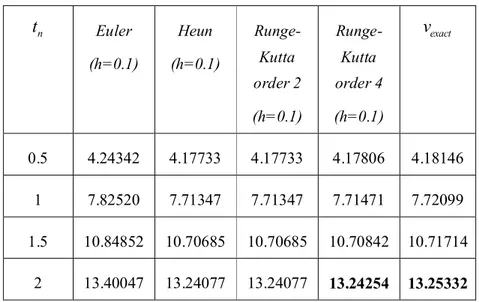
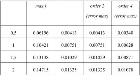
Figure 3.2.3.2.2: The table of the comparison of the given numerical methods with 0.1

h 

Figure 4.1.1.1: The table of approximation of Example 4.1.1

Figure 4.1.1.2: The table of error analysis of Example 4.1.1

Figure 4.1.2.1: The table of approximations for Example 4.1.2

xi

Figure 4.1.3.1: The table of approximation of Example 4.1.3

Figure 4.1.3.2: The table of error analysis of Example 4.1.3

Figure 4.1.3.3: The table of comparison with different step size h=0.01

Figure 4.1.3.4: The table of comparison with different step size h=0.001

Figure 4.2.1.1: The table of approximations for Example 4.2.1

Figure 4.2.1.2: The table of error analysis for Example 4.2.1

Figure 4.2.2.1: The table of approximations for t  

Figure 4.2.2.2: The table of error analysis for t  

Figure 4.2.3.1: The table of approximations for Example 4.2.3

Figure 4.2.3.2: The table of error analysis for Example 4.2.3

Figure 4.2.3.3: The comparison table of the different step size h=0.001

Figure 4.3.1.1: The table of approximations for Example 4.3.1

Figure 4.3.1.2: The table of error analysis for Example 4.3.1

Figure 4.3.2.1: The table of the temperature of the cake changing with the time

Figure 4.3.2.2: The graph of the changing the temperature of the cake with the time

Figure 4.3.2.3: The table of approximations for Example 4.3.2

Figure 4.3.2.4: The table of error analysis for Example 4.3.2

xii

Figure 4.3.2.6: The table of error analysis for Example 4.3.2

Figure 4.3.3.1: The table of approximations for Example 4.3.3

Figure 4.3.3.2: The table of error analysis for Example 4.3.3

Figure 4.3.3.3: The table of approximations with different step size h=0.001

Figure 4.4.1.1: The table of approximations for Example 4.4.1

Figure 4.4.1.2 The table of error analysis for Example 4.4.1

Figure 4.4.2.1: The table of approximations for Example 4.4.2

Figure 4.4.2.2: The table of error analysis for Example 4.4.2

Figure 4.4.3.1: The table of approximations for Example 4.4.3

Figure 4.4.3.2: The table of error analysis for Example 4.4.3

Figure 4.4.3.3: The table of approximations with different step size h=0.01

Figure 4.5.1.1: The table of approximations for Example 4.5.1

Figure 4.5.1.2: The table of error analysis for Example 4.5.2

Figure 4.5.2.1: The table of approximations for Example 4.5.2

Figure 4.5.2.2: The table of error analysis for Example 4.5.2

Figure 4.5.2.3: The table of approximations when t  

Figure 4.5.3.1: The table of numerical approximations for Example 4.5.3

xiii

xiv

INDEX OF ABBREVIATIONS

Abbreviations Explanations

RK2 Second-Order Runge-Kutta Method

RK4 Fourth-Order Runge-Kutta Method

1

1 INTRODUCTION

Mathematics is an useful subject. In society, it has applications in lots of areas such as engineering, chemistry, physics, sociology, economics and many other disciplines.

A famous mathematician once said that the complete appreciation of mathematics requires an element of poetry, and it is true that the mathematics can offer the same sort of inspiration. The poet sees the essence behind the daily experience, the universe in agrain of sand, and the mathematicians sees the law working behind the parachute and the pendelum, the suspension bridge and the rolling motion of a wheel. The law is hidden in differential equations which is a branch of mathematics. The subject of differential equations constitutes a large and very important branch of modern mathematics. In word, an equation includes unknown functions and its derivatives is called differential equation. We will give another definition of differential equations in following section. Without knowing something about differential equations and methods of solving them it is difficult to appreciate the history of this important branch of mathematics. Further the development of differential equations is intimately interwoven with the general development of mathematics and can not be seperated from it. Nevertheless to provide some historical perspective, we indicate here some of the major trends in the history of the subject and identify the most prominent early contributors (Pickles, 2010).

Isaac Newton (1642-1727) did relatively work in differential equations as such his development of the calculus and elucidation of the basic principles of mechanics provided a basis for the application in the eighteenth century, most notably by Euler. Newton classified first order differential equations according to three forms

dy/dx = f (x), dy/dx = f (y), and dy/dx = f (x, y) (Boyce andDiprima, 2001).

Gottfried Leibniz (1646-1716) was mainly self-taught in mathematics since his interest in the subject developed when he was in his twenties. Leibniz arrived at the fundamental results of calculus independently, although a little later than Newton, Leibniz was very concious of the power of good mathematical notation and was responsible for the notation dy/dx for the derivative and for the integral sign. He

2

discovered the methods of seperation of variables in 1691, the reduction of homogeneous equations to seperable ones in 1691, and the procedure for solving first order linear equations (Boyce andDiprima, 2001).

The brother Jacob (1654-1705) and Johann (1667-1748) Bernoulli did much to develop methods of solving differential equations and to extend the range of their applications. With the aid of calculus, they solved number of problems in mechanics by formulating them as differential equations (Boyce andDiprima, 2001).

From the early days of the calculus the subject has been an area of great theoretical research and practical applications, and it continues to be so in our day. This much stated, several questions naturally arise. Just what is a differential equation and what does it signify? Where and how do differential equations originate and of what use are they? Confronted with a differential equation, what does one do with it, how does one do it, and what are the results of such activity? These questions indicate three major aspects of the subject: theory, method and application (Ross, 2004).

Let us now consider briefly where, and how, such equations actually originate. In this way we shall obtain some indication of the great variety of subjects to which theory and methods of differential equations may be applied (Ross, 2004).

Differential equations occur in connection with numerous problems that are encountered in the various branches of science and engineering. We indicate a few such problems, which could easily extended to fill many pages. The problem of determining the motion of a projectile rocket, satellite, planet, charge of current in an electric circuit, the vibrations of a wire or a membrane, conduction of heat in a rod or a slab, and curves that have certain geometrical properties; the study of the rate of decomposition of a radioactive substance or the rate of growth of a population, reactions of chemicals and in economics (Ross, 2004).

The mathematical formulation of such problems give rise to differential equations. But it is not possible many time to get the exact solution for all of these problems analytically. Getting the exact solution for those types of all problems can be a challenge (Ross, 2004).

3

The numerical method is a solution technique that provides accurate approximation for the problem. The differential equations that resist solution by analytically led to the investigation of numerical methods for the problem. Therefore we need numerical methods for at least approximating the solution. Differential equations provide a rather more difficult problem. The basic method is to divide continuous time into discrete intervals, and to estimate the state of the system at the start of each interval. Thus the approximate solution changes through a series of steps. The crudest method for calculating the steps is to multiply the step length by

the derivative at the start of the interval. This method is called Euler’s method (Boyce andDiprima, 2001).

The greatest mathematician of the eighteenth century Leonhard Euler (1707-1783) was a student of Bernoulli. His interests ranged over all areas of mathematics and many fields of application. Of particular interest is his formulation of problems in mechanics. Lagrange said of Euler’s work in mechanics “The first great work in which analysis is applied to the science of movement.” Among other things Euler identified the condition for exactness of first order differential equations developed the theory of integrating factors, and gave the general solution of homogeneous linear equations with constant. (Boyce andDiprima, 2001).

In the nineteenth century interest turned more toward the investigation of theoretical questions of existence and uniqueness and to the development of less elementary methods such as those based on powerseries expansions (Boyce and Diprima, 2001).

In addition to Euler’s method, Heun’s method which is known also the modified Euler’s method is a numerical approximation method for solving ordinary differential equations. This method is named by Karl Heun (1859-1929) (Boyce andDiprima, 2001).

By 1900 fairly effective numerical integration methods had been devised, but their implementation was severely restricted by the need to execute the computations by hand or with very primitive computing equipment. In the last 60 years the development of increasingly powerful and versatile computers has vastly enlarged the range of problems that can be investigated effectively by numerical methods. Within the past few years these two trends have come together. Computers, and especially

4

computer graphics, have given a new impetus to the study of systems of nonlinear differential equations. Unexpected phenomena such as strange attractors, chaos, and fractals, have been discovered, are being intensively studied, and are leading to important new insights in a variety of applications (Boyce andDiprima, 2001).

More sophisticated techniques are presented by two German mathematicians Carl Runge (1856-1927) publishes the first Runge-Kutta method in performing the Runge-Kutta types of integration. Fourth order Runge-Kutta method that is described by Martin Kutta (1867-1944) is both commonly used and sufficiently accurate for most applications. It is always worth treating numerical solutions to differential equations with caution. Errors in calculating them may accumulate. Here, we will have the choose of numerical techniques such as Euler’s method, Heun’s Method, Second-Order Runge-Kutta and Fourth-Order Runge-Kutta (Roberts, 2010).

The study of differential equations in the twenty-first century remains a fertile source and fascinating and important unsolved problems. Finding and interpreting the solutions of these differential equations is therefore a central part of applied mathematics, and a thorough understanding of differential equations is essential for any applied mathematicians. (Roberts, 2010).

This study contains the basic concepts of differential equations such as definitions and classifications. In order to get familiar with the solution methods, both analytical and numerical methods are presented. Later on, the applications of ordinary differential equations and their numerical and analytical solutions are given. Here in this study, our first concern is approximating the solution and determining the best method for the given each problems in the light of given foregoing.

5

2 BASIC CONCEPTS IN DIFFERENTIAL EQUATIONS

Definition 2.1: An equation containing the derivatives of one or more dependent variables, with respect to one or more independent variables, is said to be a differential equation (Zill and Cullen, 2005).

Some examples of differential equations are given below

= + =

Differential equations are classified according to the specified properties that are given below

2.1 Classifications of Differential Equations

2.1.1 Classification by Type

Definition 2.1.1.1: If an equation contains only ordinary derivatives of one or more dependent variables with respect to a single independent variable it is said to be an ordinary differential equation (Zill and Cullen, 2005).

Some examples of ordinary differential equations are given below

+ 5 = + = 2 +

Definition 2.1.1.2: An equation involving partial derivatives of one or more dependent variables of two or more independent variables is called a partial differential equation (Zill and Cullen, 2005).

Some examples of partial differential equations

2 2 2 2 0 u u y x       2 2 2 2 2 u u u x t t        

2.1.2 Classification by Order and Degree

Definition 2.1.2.1: The order of a differential equation is the order of the highest derivative in the equation (Zill and Cullen, 2005).

6

Some examples of differential equations with different orders are given below

''' 2 '' ' sin y  y  y  x order: 3 2 3 2 ( y) dy lnx x dx     order: 2

Definition 2.1.2.2: The degree of a differential equation is given by the exponent that is raised the highest derivative that occurs in the equation (Ross, 2004).

Some examples of differential equations with different orders and degrees are given below − = 0 order: 1 degree: 1 2 4 2 3 ( ) 3 0 d y dy x y dx  dx   order: 2 degree: 1 ( ′′) + ( ′) − 4 = 4 + 1 order: 2 degree: 3 2.1.3 Classification by Linearity

Definition 2.1.3.1: An n-th order ordinary differential equation ( , , , … ( )) = 0 is said to be linear if F is linear in , , … ( ). This means an

n-th order ordinary differential equation is linear when ( , , , … ( )_{) = 0 is} ( ) + ( ) +...+ ( ) + ( ) − ( ) = 0 or

( ) + ( ) +...+ ( ) + ( ) = ( ) (2.1.3.1)

Two important special cases of (2.1.3.1) are linear first order and linear second order. But here we will only consider linear first order ordinary differential equations (Zill and Cullen, 2005).

In other words, in a differential equation if every dependent variables and the degree of every derivatives with any order is one and the dependent variables itself and the derivatives do not lie as multiplication then the equation is called linear differential equation (Ross, 2004).

7

Definition 2.1.3.2: A nonlinear ordinary differential equation is simply one that is not linear (Ross, 2004).

Some examples of linear and nonlinear differential equations are given below

(yx dx) 4xdy 0 linear '' 2 ' 0 y  y  y linear (1y y) ' 2 yex nonlinear 2 2 sin 0 y y x     nonlinear + 3( ) + = 0 linear

2.1.4 Classification by Type of Coefficients

Definition 2.1.4.1: A linear differential equation has constant coefficients if the coefficients of , ', '',...y y y are all constants (Ross, 2004).

Definition 2.1.4.2: A linear differential equation has variable coefficients if the , ', '',...

y y y are multiplied by any variable (Ross, 2004).

Some examples of differential equations with constant and variable coefficients are given below

'' ' 0

y  y y with constant coefficients

2 '' 2 '

xy  x y yx with variable coefficients

2.1.5 Classification by Homogeneity

Definition 2.1.5.1: For the linear differential equation

( ) + ( ) +...+ ( ) + ( ) = ( ) if ( )=0 then the equation is called homogeneous (Bronson and Costa, 2006).

8

Definition 2.1.5.2: If a differential equation is not homogeneous then it is nonhomogeneous (Bronson and Costa, 2006).

Some examples of homogeneous and nonhomogeneous differential equations are given below '' 2 ' 0 y  y y homogeneous 2 x dy x y x e dx   nonhomogeneous 2.2 Nature of Solutions

Definition 2.2.1: A function = ( ) is a solution of a differential equation if the equation is satisfied when y and its derivatives are replaced by ( ) and its derivatives (Ross, 2004).

Definition 2.2.2: A general solution to an n-th order differential equation is a solution in which the value of the constant, c in the solution, may vary (Ross, 2004).

Definition 2.2.3: Let be a real function defined for all in a real interval and having n-th derivative for all ∈ . The function is called an explicit solution of differential equation (Ross, 2004).

( , , , , … , ) = 0 (2.2.3.1)

if ( , ( ), ′( ), … , ( )) = 0 is defined for all ∈ and

if ( , ( ), ′( ), … , ( )) = 0 for all ∈ .

That is, the substitution of ( ) and its various derivatives, respectively (2.2.3.1) reduces to (2.2.3.1) an identity on (Ross, 2004).

Definition 2.2.4: A relation ( , ) = 0 is called an implicit solution of (2.2.3.1) if this relation defines at least one real function of the variable on an interval such that this function is an explicit solution of (2.2.3.1) on this interval (Ross, 2004).

An example of an explicit solution and implicit solution is given below

9

Example 2.2.4.1: Consider the function defined for all real by

( ) = 2 sin + 3 cos (2.2.4.1)

is an explicit solution of the differential equation

+ = 0 (2.2.4.2)

for all real . Observing that

′( ) = 2 − 3 and ( ) = −2 − 3 .

Substituting into the differential equation,

(−2 − 3 ) + (2 sin + 3 cos ) = 0 which holds for all real .

Thus 2.2.4.1 is an explicit solution of (2.2.4.2)

Example 2.2.4.2: The relation + − 25 = 0 (2.2.4.3) is an implicit solution of the differential equation

+ = 0 (2.2.4.4)

on the interval defined by −5 < < 5. For the relation (2.2.4.3) defines two real functions

( ) = √25 − and ( )= −√25 − respectively for all real ∈ and both of these two functions are explicit solutions of the differential equation (2.2.4.4).

Choosing ( )= √25 − and calculating ( ) =

√

for all real ∈ . Substituting ( ) and ( ) into (2.2.4.4), we obtain the identity

+ (√25 − )(

√ ) = 0 or − = 0

which holds for all real ∈ . Thus the function ( ) is an explicit solution of (2.2.4.4) on interval (Ross, 2004).

10

Definition 2.2.5: On some interval containing x₀ the problem is given as 1 ( , , ',..., ) n n n d y f x y y y dx   subject to 1 0 0 0 1 0 1 ( ) , '( ) ,..., n ( ) n y x  y y x  y y  x  y

where y y₀, ₁,...,y_n1 are arbitrarily specified real constants, is called an initial value

problem. The value x₀, 1

0 0 0 1 0 1

( ) , '( ) ,..., n ( ) n

y x y y x y y  x y



   are called inital

conditions (Zill and Cullen 2005).

In other words, if all of the associated supplementary conditions relate to one value, the problem is called initial value problem. If the conditions relate to two different values, the problem is called boundary value problem (Ross, 2004).

An example of inital value problem is given below

Example 2.2.5.1: Consider a solution for ′ = 2 at (1) = 4. Integrating both sides, we get

= +c,

where c is an arbitrary constant.Applying the initial condition we obtain = 3. Therefore

= +3,

satisfies the requirements for the initial value problem (Ross, 2004).

Example 2.2.5.2: Consider a solution for + = 0 at (0) = 1 and ( /2) = 5.

In this example we seek for a solution at two different x values, therefore it is a boundary value problem.

Since the given differential equation is a second order linear ordinary differential equation and the roots of the auxiliary equation are complex numbers.The general solution of the differential equation is

11 Applying the boundary conditions,

( ) = 5 + 3

12

3 ANALYTICAL AND NUMERICAL METHODS FOR SOLVING FIRST-ORDER ORDINARY DIFFERENTIAL EQUATIONS

The methods for solving first order ordinary differential equations can be categorized into two main title called analytical and numerical methods. Previously analytical methods were a major method for solving differential equations. These are the methods where we can get the exact solution. In order to write down solutions, we can use our knowledge of calculus, algebra and other mathematical fields,. Analytical methods are generally useful to work for simple models , however they are not enough for complex mathematical expressions that can not be solved by hand. It takes too much time to get the exact solution and sometimes it is not possible to reach to a solution.

Therefore, numerical methods are discovered. Numerical methods are the name of the methods that we get the solutions using algorithms.These methods help us to get the approximate solutions for the mathematical models, even though it is complicated. Any complex mathematical model can be solved by using computer programmes and can be executed. By using numerical methods the approximations can be nearly exact.

3.1 Analytical Methods for Solving First Order Ordinary Differential Equations

Analytical solutions are sometimes called closed-form solution or explicit solution. An equation is said to be a closed-form solution if it solves a given problem in terms of functions and mathematical operations from a given generally accepted set. These solutions are obtained by analytical methods (Edwards and Penney, 1996).

Here, numerous analytical methods are presented. There are several methods for solving ordinary differential equations. The exact results can be obtained by definite procedures with the aid of the calculus.

In this section, the methods are given for solving first order differential equations. The most general first order differential equation can be written as

( , )

dy

f x y

dx  (3.1.1)

There is no general formula for the solution to (3.1.1) but there are several classification in order to solve it. First, the equation is classified and then it can be solved.

13

Here are the numerous methods that are used for first order differential equations. (Edwards and Penney, 1996).

3.1.1 Seperable Differential Equations

The first-order differential equation dy H x y( , )

dx is called seperable provided

that H x y can be written as the product of a function of x and a function of y. ( , )

( ) ( ) dy g x h y dx   ( ) ( ) g x f y where 1 ( ) ( ) h y f y

 . In this case the variables x and y can be separated-isolated on opposite sides of an equation-by writing informally the equation.

( ) ( )

f y dyg x dx

which we understand to be concise notation for the differential equation

( )dy ( )

f y g x

dx 

It is easy to solve this special type of differential equation simply by integrating both sides with respect to x :

( ( ))dy ( ) f y x dx g x dx C dx  





equivalently, ( ) ( ) f y dy g x dx C





All that is required is that the antiderivatives.

( ) ( )

F y 

_

f y dy and G x( )

_

g x dx( ) can be found.

After doing the integrations the implicit solution that can be solved for an explicit solution is found (Edwards and Penney, 1996).

14

Remark: If the dependent and independent variables are in the case of addition or subtraction, then the equation is not seperable (Ross, 2004).

The example of seperable equations is given below

Example 3.1.1.1: Solve the initial value problem dy 6xy

dx   where (0)y  7

Solution 3.1.1.1: Informally, we divide both sides of the differential equation by

y and multiply each side by dx to get

6 dy xdx y   , (0)y  7 Hence 6 dy xdx y  





2 ln y  3x C

It is seen from the initial condition (0)y  that ( )7 y x is positive near x  , so 0 we may delete the absolute value symbols:

2 lny 3x C and hence 2 2 2 3 3 3 ( ) x C x C x y x e  e e  Ae where C

Ae . The condition (0)y  yields 7 A  , so desired solution is7

2

3

( ) 7 x

y x e

 (Edwards and Penney, 1996).

3.1.2 Homogeneous Differential Equations:

If the right-side of the equationsdy f x y( , )

dx  can be expressed as a function of

the ratio y

15

always be transformed into separable equations by a change of the dependent variable. It means dy f x y( , ) dx  is homogeneous if ( , )f x y g( )y x  or ( , )f x y h( )y x  (Ross, 2004).

Suppose that = then let

=

, then = .

Taking the derivation with respect to ,

= + = ( )

Therefore

( ) − =

It is seen that the equation can be reduced to seperable.

( ) − =

Remark: A dictionary definition of "homogeneous" is "of a similar kind or nature." Consider a differential equation of the form

n n dy p q r s

Ax y Bx y Cx y

dx

  

whose polynomial coefficient functions are "homogeneous" in the sense that each of their terms has the same total degree, m n  pq  r s K (Boyce and Diprima 2001).

The example of homogeneous equations is given below

Example:3.1.2.1: Solve the differential equation that is (x2y dx2) 2xydy0

16 Solution 3.1.2.1: 2 2 2 2 ( ) 2 2 2 dy x y x y dx xy xy xy       then 1( ) 2 dy x y dx  y x If it is written in terms of y x , and getting 1 1 ( ) 2 dy y y dx x x   

Now the equation can be written as

2 1 ( ) 1 ( ) 2 y dy _x y dx x    If y

x , then the differentiation becomes

dy d x dx dx    

Substituting into the the equation

2 1 1 ( ) 2 d x dx         Therefore, ₂ 0 1 ( ) 2 dx d x        

After some manipulations,

2 2 0 1 3 dx d x       Using substitution y x 

Seperating the variables, the solution is

2 1 1 ln ln 1 3 ln 3 3 y x c x     _{ }    . (Trench, 2001).

3.1.3 Equations Reducible to Homogeneous

17

1 1 1 2 2 2

(a Xb Yc dX) (a X b Yc dY) 0.

Since ( *a1 Xb Y dX1* ) (a2*Xb2* )Y dY 0is homogeneous equation, solving

1 1 1

a Xb Y  c and a X₂ b Y₂  c₂gives the shifting condition ( , )h k ,

X   , Yx h  y and dYk dy, dX dx where 1 1 2 2

a b

a b (Bronson and Costa

2006).

The example of an equation reducible to homogeneous is given below

Example 3.1.3.1: Solve the equation (X2Y1)dX (4X 3Y6)dY 0. Solution 3.1.3.1: The equation is not homogeneous. Therefore we need to reduce the equation into homogeneous equation.

For X 2Y  1and 4X3Y  , we get 6 X  and 3 Y 2.

Choosing the shifting as (3, 2)

3

X   x Y  y 2

Since dY dy and dX dx we can write

(x 3 2(y2) 1) dx(4(x3) 3( y2) 6) dy . 0

Simplifying the equation we get the homogeneous equation

(x2 )y dx(4x3 )y dy0.

Setting y

x , then yx.

Taking the derivations dydxxd.

18

(x2x dx) [4x3x][dxxd]0 and

2

[x2x4x3 x dx) [4x3x xd] 0

After some operations

2 2 (1 2 3 ) (4 3 ) 0 x    dxx   d  Dividing by x, we get 2 (1 2 3 )dx x (4 3 )  d .

Now it is seen that the equation is seperable

2 4 3 0 1 2 3 dx d x         





.

Integrating both sides we get

2 1 ln ln 3 2 1 ln 2 y y x c x x    _{ }      Substituting y x, we get 2 1 ln ln 3 2 1 ln 2 y y x c x x    _{ }     

(Bronson and Costa, 2006)

3.1.4 Exact Differential Equations

The general form for first order ordinary differential equation is given below

( , ) ( , ) 0

M x y dxN x y dy (3.1.4.1)

if there exists F x y( , ), which F M x    and F N y    (3.1.4.2)

19

Theorem 3.1.4.1: If M N M N are continuous , , _{y, x}   t  ,  y

interval M_y N_x and then (3.1.4.1) is exact differential equation. It means that there exist F x y( , ) which satisfy (3.1.4.2) (Bronson and Costa 2006).

Firstly, for any function g y , the function ( ) F x y( , )

_

M x y dx( , ) g y( ) satisfies the condition F M

x 

  . We plan to choose ( )g y so that

( , ) '( ) F N M x y dx g y y y        _{ } 



 (3.1.4.3) Therefore '( ) ( , ) g y N M x y dx y    

_

(3.1.4.4) So it is indeed found the desired function g y by integrating the equation ( ) (3.1.4.4). Substituting this result in equation (3.1.4.3) to obtain

( , ) ( , ) ( , ) ( , ) F x y M x y dx N x y M x y dx dy y      _  _  







as the desired function with F_xMand F_y  N (Bronson and Costa 2006).

Remark: The equation M N

y x

 

   is a necessary condition that the differential

equation be M x y dx( , ) N x y dy( , )  be exact. (Edwards and Penney, 1996). 0

The example of exact equations is given below

Example 3.1.4.1: Solve the differential equation

3 2 2

(6xyy dx) (4y3x 3xy dy) 0

Solution 3.1.4.1: Let M x y( , )6xyy3 and N x y( , )4y3x23xy2. The given equation is exact because

20 2 6 3 M x y y     = N x   Integrating F M x y( , ) x  

 with respect to x ,we get

3 2 3

( , ) (6 ) 3 ( )

F x y 

_

xyy dx x yxy g y

Then taking the derivation with respect to yand set F

y    N x y( , ). This yields 2 2 2 2 3 3 '( ) 4 3 3 F x xy g y y x xy y        

And it follows that '( )g y 4y. Hence 2 1

( ) 2

g y  y C .

Therefore, a general solution of the differential equation is defined implicitly by the equation

2 3 2

3x y xy 2y C(Bronson and Costa, 2006)

3.1.5 Equations Reducible to Exact

If M_y  N_xthen the equation is not exact. If the equation is not exact, it is necessary to construct a new function ( )f x or g y in order to get the integrating ( ) factor ( , ) x y . Finding the integrating factor in two different ways are given below

( ) M N y x f x N     

 and then ( , ) x y ef x dx( ) or

( ) M N y x g y M       and then ( , ) x y g y( )eg y dy( )

By multiplying the differential equation by integrating factor the differential equation is reduced to exact differential equation (Bronson and Costa 2006).

21

The example of non-exact equations is given below

Example 3.1.5.1: Solve the differential equation

2 2

(2x y dx) (x yx dy) 0

Solution 3.1.5.1: Calculating that M y 1 Nx 2xy1. Therefore My  Nx

which means the differential equation is not exact.

2 1 2 1 2(1 ) 2 ( 1) M N xy xy y x N x y x x xy x                f x( )

Now, the integrating factor ( , ) x y can be found by using ( )f x

2

( ) _{2ln 2}

( , )

_{x y}

_e

f x dx

_e

xdx

_e

x

_x





















Multiplying both sides by 2 x

,

2 2 2 2

(2 ) ( ) 0

x x y dx x  x y x dy  ,

and organizing the equation,

2

1

(2 y)dx (y )dy 0

x x

   

Realizing that the differential equation is exact.

2 2 1 1 y x M N x x   

Now, we observe that the differential equation is reduced to exact form.

According to exact differential equation procedure

2 ( , ) (2 y)

f x y dx

x

22 Integrating the equation

1 1 '( , ) 2 y ( ) '( ) F x y x y y y x  x  x         . Therefore 2 '( ) ( ) 2 y y y y c     

The general form of the equation is found as

2 ( , ) 2 2 y y F x y x c x     (Trench, 2001).

3.1.6 First Order Linear Differential Equations

In Section (3.1.1) it was seen how to solve a separable differential equation by integrating after multiplying both sides by an appropriate factor. For instance, to solve the equation.

dy 2xy

dx  (3.1.6.1)

Multiplying both sides by the factor 1

y to get 1 2 dy x y dx (3.1.6.2)

Because each side of the equation in (3.1.6.2) is recognizable as a derivative (with respect to the independent variable x), all that remains are two simple integrations, which yield ln yx2C. For this reason, the function ( )y 1/yis called an integrating factor for the original equation in (3.1.6.1)

An integrating factor for a differential equation is a function ( , ) x y such that the multiplication of each side of the differential equation by ( , )x y yields an equation in which each side is recognizable as a derivative. With the aid of the appropriate integrating factor, there is a standard technique for solving the linear first-order equation.

23

( ) ( )

dy

P x y Q x

dx  (3.1.6.3)

on an interval on which the coefficient functions. P x and ( ) Q x are continuous. ( ) Multiplying each side of in equation (3.1.6.3) by the integrating factor.

( ) ( )x e P x dx    The result is ( ) ( ) ( ) ( ) ( ) P x dx dy P x dx P x dx e P x e y Q x e dx  _  _  _(3.1.6.4) Because [ ( ) ] ( ) x D

_

P x dx P x

The left-hand side is the derivative of the product y x e( ) P x dx( ) so equation (3.1.6.4) is equivalent to

( ) ( )

[ ( ) P x dx] ( ) P x dx

x

D y x e Q x e

Integration of both sides of this equation gives

( ) ( )

( ) P x dx ( ( ) P x dx)

y x e 

_

Q x e dx C

Finally, solving for y, we obtain the general solution of the linear first-order equation in

y x( )eP x dx( ) [ ( ( )

_

Q x eP x dx( ) )dx C ] (Edwards and Penney, 1996). The example of first order linear equations is given below

Example 3.1.6.1: Solve the inital value problem

/ 3 11 8 x dy y e dx    (0)y   1

Solution 3.1.6.1: Here, ( )P x   and 1 11 / 3 ( )

8 x

Q x e

 so the integrating factor is

( 1)

( )x e dx e x

   

24

Multiplication of both sides of the given equation by x

e yields 4 / 3 11 8 x dy x x e e y e dx      which is recognized as 11 4 / 3 8 x x d e y e dx   

Hence integration with respect to x gives

4 / 3 4 / 3 11 33 8 32 x x x e y 

_

e dx  e C and multiplication by x

e gives the general solution

/ 3 33 ( ) 32 x x y x Ce e  

Substitution of x  and 0 y   now gives 1 1 32

C  so the desired solution is

/ 3 / 3

1 33 1

( ) ( 33 )

32 32 32

x x x x

y x  e  e  e  e (Edwards and Penney, 1996).

3.1.7 Special Types of Differential Equations

We now consider a special type of equation that can be reduced to a linear equation after appropriate substitution.

3.1.7.1 Bernoulli Equations

A first order ordinary differential equation of the form

dy p x y( ) g x y( ) n

dx  (3.1.7.1)

is called a Bernoulli equation.

If n  , then Bernoulli equation is actually a linear equation or 0 n  , then 1 Bernoulli equation is seperable. However if n  or 0 n  , we must proceed in a 1 different manner.

25

Suppose that n  or 0 n  . Then we need to use the transformation 1 vy1 n .

We first multiply (3.1.7.1) by yn

, therefore we express the equation as

1 ( ) ( ) n dy n y y p x g x dx     (3.1.7.2) If we let vy1 n , then (1 ) n dv dy n y dx dx   

Substituting the variables, (3.1.6.2) transforms to

1 ( ) ( ) 1 dv p x v g x n dx   equivalently, (1 ) ( ) (1 ) ( ) dv n p x v n g x dx     Letting p x₁( )(1n p x) ( ) and g x₁( )(1n g x) ( )

The equation may be written as

1( ) 1( )

dv

p x v g x

dx 

which is linear in v (Ross, 2004).

The example of Bernoulli Equation is given below

Example 3.1.7.1.1: Solve dy 3

y xy

dx  .

Solution 3.1.7.1.1: This problem is a Bernoulli differential equation where n 3 .

26

We first multiply the equation by y3. Therefore we obtain

3dy 2

y y x

dx

 

  .

Substituting vy1 n  y1 3  y2, and differentiating dv 2y 3dy

dx dx



  .

Preceeding the differential equation reduces to the linear equation as

1 2 dv v x dx   

Writing the equation in the standard form

2 2

dv

v x

dx   (3.1.7.1.1)

The integrating factor is

( ) 2 ₂ p x dx dx _x e e e Multiplying (3.1.7.1.1) by 2 x e , 2 2 2 2 2 x dv x x e e v xe dx       Integrating, we find 2 1 2 (2 1) 2 x x e v e x  c

Simplifying the equation we find

where c is an arbitrary constant.

2 1 2

x

27 Replacing v 1₂ y  , we get 2 2 1 1 2 x x ce y    (Ross, 2004) 3.1.7.2 Riccati Equation

Suppose that ( )P x , Q x and ( )( ) R x are continuous functions.

2

( ) ( ) ( )

dy

P x y Q x y R x

dx  

is the general form of Riccati equation.

The general solution for this equation can not be found by directly, but if they give one or more special solution we can find the general solution.

If yy x₁( ) is the special solution for Riccati diffential equation, then the general solution;

( ) ( )

y z x  y x

where zis the dependent and x is the independent variable then the equation can be reduced to Bernoulli equation, or,

1 1 ( ) ( ) y y x u x  

where u is the dependent and x is the independent variable then the equation can be reduced to linear equation (Bronson and Costa 2006).

Example 3.1.7.2.1: Given Riccati equation

2

( ) ( )

dy

P x y y R x

dx   for two special solution y1 x and y2  x 1.

28 Solution 3.1.7.2.1: Since 1 y  x, then dy₁dx or 1 1 dy dx  . Therefore 2 ( ) ( ) ( ) dy P x y Q x y R x dx   2 1P x x( ) x R x( ) (3.1.6.2.1) 2 1 y  x , then dy₂ dx or 2 1 dy dx  . Therefore, 2 1P x x( )( 1)(x1) R x( ) (3.1.7.2.2)

Solving the equations (3.1.7.2.1) and (3.1.7.2.2) together , we have

( ) 2 1 P x  x and R x( )x2 x 1 Therefore, 2 2 (2 1) 1 dy x y y x x dx      (3.1.7.2.3)

Since y₁ x, then y  and taking the derivation 'z x y  z' 1 .

Substituting into the (3.1.7.2.3),

2 2

' 1 (2 1).( ) ( ) 1

z  x zx  zx x  x

After some operations we have,

If z' z z2 then dz 2

z z

dx  ,

29 2 1 ' 1 z z z  Substituting now , 1 z  then v v' z z2 ', we obtain ' 1 v v    or 'v   . v 1

Here, we realize that the equation is linear differential equation. Applying the linear differential equation procedures we have

[ .( 1) ] dx dx

ve

_

e  dx

After some manipulations

( ) x x ve e c Replacing with z, 1 ( ) x x e e c z     Since z  yx, 1 ( ) x x e e c y x    

 (Bronson and Costa 2006).

3.1.7.3 Clairout Equation

' ( ')

yxy  f y

is the general form of Clairout equation. The general solution for this equation is

( )

ycx f c .

If we substitute 'y  p into the equation,

( )

yxp f p

First derivation of x can be obtained as

' dp dp '( )

y p x f p

dx dx

  

30 '( ) dp dp p p x f p dx dx    equivalently, 0xp' p f' '( )p Therefore '( '( )) 0 p x f p  Here, we obtain p ' 0 or x f '( )p  0

If p ' 0, then 'y  and c yxc f c( ) is the general solution.

If x f '( )p  , then 0 pcan be solved as a function of x and yxp f p( ) is singular solution (Bronson and Costa 2006).

Example 3.1.7.3.1: Find the singular and general solution of the problem 2

' ' ( ')

yxyy  y .

Solution 3.1.7.3.1: Here we realize that the equation is Clairaut equation. Substituting 'y  p,

2

yxppp

and the derivation is

' ' ' 2 ' y  pxp p  pp Substituting again 'y  p ' ' 2 ' p pxp p pp Therefore '( 1 2 ) 0 p x  p 

31 Here we have p ' 0 or x 1 2p0

For p ' 0, p c then ycx x c  2 is the general solution.

For x 1 2p , then 0 yxppp2.

Using x2p , 1 yxppp2 is reduced to y(2p1)ppp2.

Simplifying the equation, we obtain yp2.

Therefore ( 1 )2 2

x

y  ,

equivalently 4y(x1 )2 is the singular solution (Bronson and Costa 2006).

3.2 Numerical Methods for Ordinary Differential Equations

In Section (3.1), we examined to solve first order ordinary differential equations analytically. As an alternative to analytical methods, we can consider the use of numerical methods. Because sometimes a solution of a differential equation may not be able to getit analytically. Numerical methods are techniques by which mathematical problems are formulated so that they can be solved with hand. The role of numerical methods in mathematical models has increased efficiently with the development of fast and efficient computers. Using any computer programming language, a numerical method can be reduced to a numerical algorithm which is a set of rules for solving a problem in finite number of steps. The numerical algorithms can be easily implemented to any mathematical models. Therefore we conclude this chapter with a method by which we can solve the differential equations numerically. We are going to mention about the well-known and basic numerical methods such as Euler, Heun and second order Kutta(RK2) and fourth order Runge-Kutta(RK4).

3.2.1 Euler’s Method (Tangent Line Method)

It is the exception rather than the rule when a differential equation of the general form

( , )

dy

f x y dx 

32

can be solved exactly and explicitly by elementary methods. For example, consider the simple equation

2 x dy e dx   (3.2.1.1)

A solution of equation (3.2.1.1 ) is simply an antiderivative of ex2

. But it is known that every antiderivative of ( ) x2

f x e

 is a nonelementary function. function-one that cannot be expressed as a finite combination of the familiar functions of elementary calculus. Hence no particular solution of equation (3.2.1.1) is finitely expressible in terms of elementary functions. To find a simple explicit formula for a solution of (3.2.1.1 ) is doomed to failure. As a possible alternative, an old-fashioned computer plotter can be programmed to draw a solution curve that starts to the inital point ( ,x y_{0 0})and attempts to thread its way through the slope field of a given differential equation y' f x y( , ).The procedure the plotter carries out can be described as follows (Edwards and Penney, 1996).

• The plotter pen starts at the initial point ( ,x y_{0 0}) and moves a tiny distance along the slope segment though( ,x y_{0 0}). This takes it to the point( ,x y_{1 1}).

•At( ,x y_{1 1})the pen changes direction, and now moves a tiny distance along the slope segment through this new starting point( ,x y_{1 1}). This takes it to the next starting point

2 2 ( ,x y ).

•At ( ,x y_{2 2})the pen changes direction again, and now moves a tiny distance along the slope segment through.( ,x y_{2 2})This takes it to the next starting point ( ,x y_{3 3}) (Edwards and Penney, 1996).

33

Leonhard Euler--the great 18th-century mathematician for whom so many mathematical concepts, formulas, methods, and results are named did not have a computer plotter, and his idea was to do all this numerically rather than graphically. In order to approximate the solution of the initial value problem

( , )

dy

f x y

dx  y x( )0 y0 (3.2.1.2)

First, choosing a fixed (horizontal) step size h to use in making each step from one point to the next. Suppose that it is started at the initial point ( ,x y_{0 0})and after n

steps have reached the point ( ,x y_{n n}).Then the step from( ,x y_{n n})to the next point 1 1

(x_n ,y_n) is illustrated in Figure (3.2.1.2).

Figure 3.2.1.2: The step from( ,x y_{n n}) to (x_n1,y_n1)

The slope of the direction segment through( ,x y_{n n}) is m f x y( ,_{n n}). Hence a horizontal change of h fromx_nto x_n1 corresponds to a vertical change of

. . ( ,_{n n})

m hh f x y fromy_n toy_n1.

Therefore the coordinates of the new point (x_n1,y_n1)are given in terms of the old coordinates by

1

n n

x_ x h y_n1y_nhf x y( ,_{n n}) (3.2.1.3)

Given the initial value problem in (3.2.1.2), Euler's method with step size h consists of starting with the initial point ( ,x y_{0 0})and applying the formulas

1 0

34 2 1 x x h y₂ y₁h f x y. ( ,_{1 1}) 3 2 x x h y3y2h f x y. ( ,2 2) . . . . . .

to calculate successive points ( ,x y_{1 1}), ( ,x y_{2 2}), ( ,x y_{3 3}),…on an approximate solution curve.(Edwards and Penney, 1996).

Example 3.2.1.1: Apply Euler's method to approximate the solution of the initial value problem 1 5 dy x y dx  (0)y   3

(a) first with step size h  on the interval [0,5] , 1 (b) then with step size h 0.2on the interval [0,1] .

Solution 3.2.1.1: (a) With x ₀ 0, y  ₀ 3, ( , ) 1 5

f x y x yand h  the iterative 1 formula in (3.2.1.2) yields the approximate values

1 0 0 0 1 [ ] 5 y  y h x  y =( 3) (1)(0 1( 3) 3.6 5       _{2 1} [ ₁ 1 ₁] ( 3.6) (1)(1 1( 3.6) 3.32 5 5 y y h x  y        _{3 2} [ ₂ 1 ₂] ( 3.32) (1)(2 1( 3.32) 1.984 5 5 y  y h x  y        _{4 3} [ ₃ 1 ₃] ( 1.984) (1)(3 1( 1.984) 0.6192 5 5 y y h x  y       _{5 4} [ ₄ 1 ₄] (0.6192) (1)(4 1(0.6192) 4.7430 5 5 y y h x  y    

35

at the points x ₁ 1, x ₂ 2, x ₃ 3, x ₄ 4, x ₅ 5. Note how the result of each calculation feeds into the next one. The resulting table of approximate values is

x ₀ 1 2 3 4 5

.

Approx y 3 3.6 3.32 1.984 0.6192 4.7430

Figure:3.2.1.3: The table of approximations with Euler’s method when h 1

(b) Starting a fresh with x ₀ 0,y  ₀ 3, ( , ) 1 5

f x y x y the approximate values are 1 0 0 0 1 1 [ ] ( 3) (0.2)[0 ( 3)] 3.12 5 5 y  y h x  y        _{2 1} [ ₁ 1 ₁] ( 3.12) (0.2)(0.2 1( 3.12) 3.205 5 5 y y h x  y        _{3 2} [ ₂ 1 ₂] ( 3.205) (0.2)(0.4 1( 3.205) 3.253 5 5 y  y h x  y        _{4 3} [ ₃ 1 ₃] ( 3.253) (0.2)(0.6 1( 3.253) 3.263 5 5 y y h x  y        _{5 4} [ ₄ 1 ₄] ( 3.263) (0.2)(0.8 1( 3.263) 3.234 5 5 y  y h x  y       

At the pointsx ₁ 0.2, x ₂ 0.4, x ₃ 0.6, x ₄ 0.8 and x ₅ 1.

x _{0 0.2 0.4 0.6 0.8} 1

.

Approx y 3 3.12 3.205 3.253 3.263 3.234

Figure 3.2.1.4: The table of approximation when h 0.2

Figure 3.2.1.5 shows the graph of this approximation, together with the graphs of the Euler approximations obtained with step sizesh 0.2and 0.05, as well as the graph of the exact solution.