Optimum Method for Determining Weibull Distribution Parameters Used in Wind Energy Estimation 635
Optimum Method for Determining Weibull
Distribution Parameters Used in Wind Energy
Estimation
Nil Aras1, Ulku Erisoglu2*, Hasan D. Yıldızay3
* Corresponding Author
1. Eskişehir Technical University, Engineering Faculty, Department of Industrial Engineering, Eskişehir, 2655, Turkey, nila@Eskişehir.edu.tr
2. Necmettin Erbakan University, Department of Statistics, Faculty of Science, Konya, 42090, Turkey,
3. Dumlupınar University, Engineering Faculty, Department of Mechanical Engineering, Kütahya, 43100, Turkey, [email protected]
Abstract
One of the well-known methods for the determination of wind energy potential is the two-parameter Weibull distribution. It is clear that the success of the Weibull distribution for wind energy applications depends on the estimation of the parameters which can be determined by using various numerical methods. In the present study, Monte Carlo simulation method is performed by using six parameters estimation method that is used in the estimation of Weibull distribution parameters such as Maximum Likelihood Estimation (MLE), Least Squares Method (LSM), Method of Moments (MOM), Method of Logarithmic Moments (MLM), Percentile Method (PM), and L-Moment Method (LM), and is compared to Mean Squared Error (MSE) and Mean Absolute Percentage Error (MAPE). In this study, the wind energy potential of the Meşelik region in Eskişehir was modeled with two-parameter Weibull distribution. The average wind speed (m/s) data, which are gathered in 10-minute intervals from the measuring device installed 10 meters about the ground in Meşelik Campus of Eskişehir Osmangazi University, is used. As a result of the simulation study, it has been determined that MLE is the best parameter estimation method for two-parameter Weibull distribution in large sample sizes, and LM has the closest performance to MLE. The wind speed (m/h) data of the region has been successfully modeled with two-parameter Weibull distribution and the highest average wind power density has been obtained in July as 49.38295 (W/m2) while the lowest average wind power density has been obtained in October as 19.30044 (W/m2).
Key Words: Wind speed; Wind Power Density; Weibull Distribution; Maximum Likelihood Method; L-Moment
Method; Wind Data.
Mathematical Subject Classification: 62F10 1. Introduction
In converting the wind potential to electrical energy, the wind speed distribution in the turbine installed area plays an important role along with wind turbine parameters. In the design of the system that will optimize the energy generation costs in practice, correct modeling of the wind regime in the area is crucial. The most commonly preferred method for the modeling of the frequency distribution of wind speeds is the Weibull distribution. Examining the literature, there are several studies in which the wind potential of an area is determined through Weibull distribution (by Carta et al., 2009). Literature research indicates that many studies have been carried out to determine wind energy potential in different regions through the Weibull distribution. The following were given a few studies in which wind energy potential was determined by the Weibull distribution.
The study carried out by Baseer et al. (2017) indicates the wind characteristics of seven sites in Jubail, Saudi Arabia through the Weibull distribution function. Within their study, they have collected five years’ wind data from six locations and three years’ data from one location both of which have been gathered at a height of 10 meters. Baseer
Optimum Method for Determining Weibull Distribution Parameters Used in Wind Energy Estimation 636 et al. (2017) have utilized the maximum likelihood, the least-squares methods, and the WASP algorithm to determine the parameters of the Weibull distribution. They have indicated that the maximum likelihood method is better than others in the prediction of the Weibull parameters. Novoa et al. (2017) have analyzed the daily wind speed data collected from 46 automatic weather stations in Navarre, northern Spain via Weibull distribution. They have indicated that 23% of the regions had adequate wind resources for the installation of wind turbines. Shoaib et al. (2017) have analyzed wind speed data gathered at five different heights through Weibull distribution at Baburband. They have expressed that the region has 278 W/m2 wind power potential at Baburband site. Wais (2017) has compared 2 and 3 parameter Weibull distributions in order to design a model for wind speed data in the 3 different turbine sites. The results have indicated that for the higher likelihood of the null wind, the 3-parameter Weibull distribution yields better results compared to the 2-parameter Weibull distribution. Akdağ and Güler (2018) have offered a new method called alternative moment method for estimating the Weibull parameters in the assignation of the wind energy potential. They have compared the efficacy of the offered method with commonly used parameter estimation methods. The comparison has indicated that the offered method is better than Justus moment and novel energy pattern factor methods. Furthermore, they have predicted the wind energy potential data collected from 16 different weather stations located around Spain through the offered method. Soulouknga et al. (2018) have calculated the wind energy potential of Faya-Largeau via the Weibull distribution for the wind speed data gathered at 10 meters height. They have predicted that the annual values of the Weibull shape and scale parameters are respectively 3.75 and 3.60 (m/s) while the power density and available energy are 343.31 W/m2 and
249.87 kWh/m2, respectively. Ali et al. (2018) have predicted the wind energy potential of the Deokjeok-do Island –
Incheon (South Korea) via Weibull distribution. They have utilized the wind data gathered at 10 meters’ height, including wind speed and wind direction for 17 years (2000–2016). Kantar et al. (2018) have come up with the extended generalized Lindley distribution as an alternative to the Weibull distribution to assess wind energy potential. They have analyzed the performance of the offered alternative distribution method for the wind speed data collected at four stations in Turkey.
Wind speed and direction data are needed to determine the wind energy potential of a site for energy generation purposes. Therefore, the wind speed and direction values should be measured periodically in conformity with the standards by installing wind measurement station(s) in a suitable place or places in the region. Wind energy is predominantly a nonsynchronous generation source. The project design and economy of the wind power plant depend mainly on the amount of energy that could be generated at the selected plant site. Wind power curves play important roles in wind power forecasting. In order to determine this amount of energy, the data obtained from the wind measurements made in the energy production regions should be analyzed statistically (by Malvaldi et al., 2017). As a result of this analysis, a very important infrastructure will be formed for the wind turbines to be installed in the region by determining the annual average wind speed, dominant wind direction, average power density of the region (by Aras, 2003).
This study mainly aims to discover the wind potential of the region of Meşelik in Eskişehir through analyzing the wind data gathered between July 2013 and June 2014. The wind energy potential of the Meşelik region has been evaluated through two-parameter Weibull distribution in this study. In previous studies, where wind potential is analyzed by Weibull distribution, wind speed measurements obtained at a height of 10 meters were generally used. Therefore, in the evaluation of the wind potential of the area, the wind speed (m/h) data gathered in 10 minute intervals from the measuring device installed 10 meters above ground in the Meşelik Campus of Osmangazi University were used.
Within the study, a simulation study was carried out first to determine the optimal parameter estimation method in the estimation of Weibull distribution parameters. In the comparison of the estimation methods, mean square error (MSE) and mean absolute percentage error (MAPE) criteria were used. Following the selection of the most suitable parameter estimation method, the average wind speed (m/h) data obtained during the period July 2013-June 2014 were modeled by month with two-parameter Weibull distribution. The wind characteristics calculated based on the obtained parameter Weibull distribution were compared with wind characteristics calculated based on the observation. Moreover, the compliance of wind speeds with two-parameter Weibull distribution modeling, were evaluated with the root of mean square error (RMSE) and the coefficient of determination (R2) criteria.
The rest of this study is organized as follows: two-parameter Weibull distribution and wind characteristics based on two-parameter Weibull distribution are defined in the section 2. The six different parameter estimation methods for two-parameter Weibull distribution are presented in the section 3. Comparison of the parameter estimation methods
Optimum Method for Determining Weibull Distribution Parameters Used in Wind Energy Estimation 637 using the Monte Carlo simulation method is given in section 4. The details about the data used for analysis and results derived from this study are discussed in section 5. Finally, some conclusions are noted in section 6.
2. Weibull Distribution
Probability density function (pdf) of two-parameter Weibull distribution is shown with the equation below: fwbl(v) = k c( v c) k−1 exp [− (v c) k ] (1)
In Eq. 1; v represents observed wind speed, and c and k represent scale and shape factors, respectively. Cumulative Distribution Function (CDF) of Weibull is given in Eq. 2.
Fwbl(v) = 1 − exp [− (
v c)
k
] (2)
In the modeling of wind speed (m/h) data with two-parameter Weibull distribution, the mean wind speed and the standard deviation of the wind speeds that are determined based on two-parameter Weibull distribution are shown in Eqs. 3 and 4. v̅wbl= cΓ (1 + 1 k) (3) σwbl= {c2[Γ (1 + 2 k) − Γ 2(1 +1 k)]} 1 2 (4)
The Γ(. ) in Eqs. 3 and 4 represent the gamma function. As is known, the wind power potential of a wind turbine at v speed with a wing swept area of A is calculated as shown in Eq. 5.
P(v) =1 2ρAv
3 (5)
In Eq. 5; ρ; is the air density and is calculated as 1.225 kg/m3. Mean power density for two-parameter Weibull
distribution is obtained with Eq. 6 below. Pwbl=
1 2ρc
3Γ (1 +3
k) (6)
3. Parameter Estimation Methods
Forecasting for wind energy is becoming more important as the amount of energy generated from wind increases (by Sweeney, 2020). In determining the wind energy potential of an area based on two-parameter Weibull distribution; firstly, c and k should be estimated. Numerous methods have been developed to estimate the parameters of two-parameter Weibull distribution. In this study; most commonly used methods, which are maximum likelihood estimation (MLE), least squares method (LSM), method of moments (MOM), method of logarithmic moments (MLM), percentile method (PM), and L-moment method (LM), will be examined.
3.1. Maximum Likelihood Estimation (MLE)
The log-likelihood function for two-parameter Weibull distribution is given by lnL = nlnk − nklnc + (k − 1) ∑ lnvi n i=1 − c−k∑ v ik n i=1 (7)
Optimum Method for Determining Weibull Distribution Parameters Used in Wind Energy Estimation 638 In order to obtain the maximum likelihood estimations of two-parameter Weibull distribution, a log-likelihood function given in Eq. (7) must be derived according to parameters c and k, respectively, and equations obtained by equating them to zero must be solved.
∂lnL ∂c = −nkc −1+ kc−k−1∑ v ik n i=1 = 0 (8) ∂lnL ∂k = nk −1− nlnc + ∑ lnv i+ c−klnc ∑ vik n i=1 n i=1 − c−k∑ v ik n i=1 lnvi= 0 (9)
Consequently, k̂ is obtained as the solution of
k = [∑ vi klnv i n i=1 ∑ni=1vik −∑ lnvi n i=1 n ] −1 . (10)
Despite the fact that the analytical solution is not present, k̂ could be readily solved through the iterative methods. In order to obtain the maximum likelihood estimation of k parameter of Weibull distribution, the Newton-Raphson method could be used (by Genc et al., 2005). In the (r + 1)th iteration of Newton-Raphson method, maximum
likelihood estimation of k shape parameter of Weibull distribution is obtained by the equation below. k̂(r+1)= k̂r+
Ar+ (1 k̂⁄ r) − (Cr⁄ )Br
(1 + k̂r2) + (BrDr− Cr2) B⁄ r2
(11)
Terms in Eq. 11 are defined as Ar= ∑ni=1lnvi⁄ , Bn r= ∑ vi k ̂r n i=1 , Cr= ∑ vi k ̂r lnvi n i=1 and Dr= ∑ vi k ̂r (lnvi)2 n i=1 . Once
k is estimated, the maximum likelihood estimation of c is obtained as follows:
ĉ = (∑ vi k ̂ n i=1 n ) 1 k⁄̂ (12)
3.2. Least Squares Method (LSM)
Least squares estimations of two-parameter Weibull distribution parameters are obtained by using the linear relationship in Eq. (13) obtained by considering the natural logarithm of CDF in Eq. (2) twice.
ln(− ln{1 − Fwbl(vi)}) = k ln(vi) − kln (c) (13)
When the term ln(− ln{1 − Fwbl(vi)}) in Eq. (13) is defined as yi, the least-squares estimates of shape and scale
parameters of the Weibull distribution are respectively as follows;
k̂ =n ∑ ŷiln(vi) − ∑ ln(vi)
n
i=1 ∑ni=1ŷi n i=1 n ∑ni=1ln(vi)2− {∑ni=1ln(vi)}2 (14) ĉ = exp (∑ ln(vi) n i=1 n − ∑ni=1ŷi k̂n ). (15)
The term ŷi in Eqs. 14 and 15 is the estimated value obtained by using the cumulative distribution function instead
of the Fwbl(vi) in yi= ln(− ln{1 − Fwbl(vi)}) equation. In this study, the median rank value (i − 0.3)/(n + 0.4)
Optimum Method for Determining Weibull Distribution Parameters Used in Wind Energy Estimation 639
3.3. Method of Moments (MOM)
Parameter estimations in the method of moments are carried out by solving the equations obtained by equating the sample moments as many as unknown parameters to the population moments (by Karakoca et al., 2015). The first two raw moments of two-parameter Weibull distribution are defined as M1= cΓ(1 + 1 k⁄ ) and M2= c2Γ(1 +
2 k⁄ ). The first two raw moments based on a sample are calculated with m1= (∑ni=1vi)/n and m2= (∑ni=1vi2)/n
equations. The moment’s estimation of k is obtained by solving the Eq. (16): M12 M2 −m1 2 m2 = 0 (16)
Newton-Raphson, an iterative method, can be used for solving Eq. (16). In the (r + 1)th iteration of
Newton-Raphson method, moments estimation of k shape parameter of Weibull distribution is obtained with the equation below.
k̂r+1= k̂r−
Pr
Qr
(17)
The terms Pr and Qr are defined as
Pr= Γ2(1 + 1 k̂⁄ ) Γ(1 + 2 k̂⁄ ) − m12 m2 (18) Qr= 2Γ2(1 + 1 k̂ r ⁄ ){ψ(1 + 2 k̂⁄ ) − ψ(1 + 1 k̂r ⁄ )}r k̂r2Γ(1 + 2 k̂⁄ )r (19)
respectively, where ψ(. ) is the digamma function. Moment’s estimation of c scale parameter of Weibull distribution is calculated with Eq. (20) below.
ĉ = m1
Γ(1 + 1 k̂⁄ ) (20)
3.4. Method of Logarithmic Moments (MLM)
The method of logarithmic moments is a special form of the method of moments. Logarithmic moment’s estimates of two-parameter Weibull distribution parameters are obtained as shown below (by Teimouri et al., 2013).
k̂ = (π 2 6S2) 1 2⁄ (21) ĉ = exp (k̂x̅ + γ k̂ ) (22)
In Eqs. 21 and 22, S2 and x̅ are sample variance and the sample mean, respectively, for transformed data obtained by
taking the natural logarithm of wind speed data. Also, the term γ shows the Euler constant.
3.5. Percentile Method (PM)
In two-parameter Weibull distribution, the quantile function that gives the equivalent wind speed value of cumulative distribution function p is defined with the equation below
Optimum Method for Determining Weibull Distribution Parameters Used in Wind Energy Estimation 640 Percentile estimations of two-parameter Weibull distribution are obtained by equating the equations of two selected p values in quantile function to relevant observed wind speed. Percentile estimation of c scale parameter of Weibull distribution could be simply obtained by selecting p = 1 − exp(−1) ≅ 0.632 in Equation (23).
ĉ = v1−exp (−1) (24)
The percentile estimation of k is obtained with the equation below: k̂ = (ln[−ln(1 − p)]
ln(vp) − ln(ĉ)
) (25)
where 0 < vp< v0.632 should be taken (by Marks, 2005). There are several proposals for the determination of the
optimum value of p in Eq. (25). In the present study, p = 0.15 value, proposed by Wang and Keats (1995) has been used.
3.6. L-Moment Method (LM)
The L-moment estimation method is based on the rth moment of ith order statistics. As with the method of moments,
parameter estimations are performed by solving the equations obtained by equating population L-moments to sample L-moments (by Erisoglu and Erisoglu, 2014). Population L-moment μr0 is defined as in Eq. (26).
μr0= 1 r∑(−1) kC kr−1E(Xr−k:r) r−1 k=0 r = 1, 2,3, … (26)
In Eq. 24; Cin= n!/(i! (n − i)!) shows the binomial coefficient and the term Xi:n shows ith order statistics in n
sample size. Sample L-moments are calculated with the equation below.
mr0= 1 r∑ ∑ (−1)kC kr−1Ckn−iCr−k−1i−1 r−1 k=0 Crn n i=1 Xi:n (27)
L-moment estimations of shape (k) and scale (c) parameters are obtained as below, respectively.
k̂ = ln (2) ln (1 −m20 m10 ) (28) ĉ = m1 0 Γ(1 + 1/k̂) (29)
In Eqs. 26 and 27; m10 and m20 are sample L-moments and calculated using m10= ∑ni=1vi:n
n and m2 0= 2 ∑ni=1(i−1)vi:n
n(n−1) − m1
0 equations.
4. Simulation
In this part, the performances of examined parameter estimation methods in the estimation of Weibull distribution parameters have been compared with the simulation study. In the simulation study, 10.000 data sets have been generated from two-parameter Weibull distribution for the selected parameter values and different sample sizes (n = 10, 30, 50 ve 100). The chosen parameter values are decided according to parameter prediction values which are prevalent in the literature. In the Newton-Raphson iterations, the number of iterations is not restricted, and for convergence, the difference between 2 successive predictions is supposed to be smaller than 10−4 value.
Optimum Method for Determining Weibull Distribution Parameters Used in Wind Energy Estimation 641 Comparing the performances of parameter estimation methods, MSE and MAPE criteria are taken into consideration. MSE and MAPE values are respectively defined with equations below.
MSE(θ) = 1 10000∑ (θ − θ̂i) 2 10000 i=1 (30) MAPE(θ) = 1 10000∑ 100|θ − θ̂i| θ 10000 i=1 (31)
In Eqs. 30 and 31; the term θ indicates one of the unknown parameters of Weibull distribution (c and k), and the term θ̂i indicates the estimated value of the unknown θ parameter in the ith step of the simulation. The lower MSE
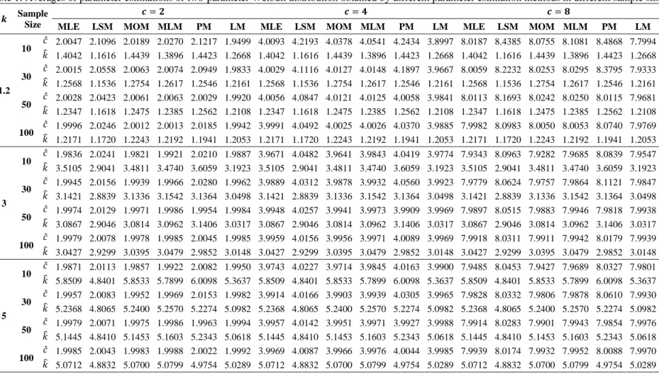
and MAPE values' means that the parameter estimation method has a good efficiency. The codes of the present study comparing the parameter estimation methods for two-parameter Weibull distribution are written in MATLAB software. Averages of parameter estimations obtained by different parameter estimation methods in different sample sizes have been presented in Table 1.
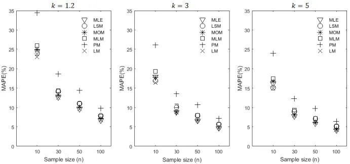
Examining Table 1; the efficiency of parameter estimation methods increases as the sample size volume increases, and averages of parameter estimations are observed to converge closer to actual parameter values. The comparison of parameter estimation methods for two-parameter Weibull distribution for different 𝑘 parameter values to average of MAPE values calculated for two-parameters of the distribution is presented in Figure 1.
Figure 1: The comparison of parameter estimation methods with the mean MAP criteria
Examining the Figure 1; according to the mean MAPE criterion, in small sample size(𝑛 = 10), LM method is seen to have better performance than other parameter methods. In other sample sizes(𝑛 = 30, 50 𝑣𝑒 100), MLE method is the most successful parameter estimation method according to mean MAPE criterion. According to the MAPE criterion, the performance of the PM method was found significantly poor than other parameter estimation methods. According to the MAPE criterion, LM parameter estimation method is considered as the best alternative for MLE method.
The averages of the MSE values obtained for parameters of the distribution with different parameter estimation methods for two-parameter Weibull distribution in different sample sizes are presented in Table 2. Examining Table 2; according to the mean MSE criterion, LM method in small sample sizes, and MLE method in large sample sizes are found to be the best performing methods in parameter estimations of two-parameter Weibull distribution. As a result of the simulation study; it is determined that MLE is the best parameter estimation method for parameter estimation of two-parameter Weibull distribution in large sample sizes, and LM has the closes performance to MLE.
Optimum Method for Determining Weibull Distribution Parameters Used in Wind Energy Estimation 642
Table 1: Averages of parameter estimations of two-parameter Weibull distribution obtained by different parameter estimation methods in different sample sizes
𝒌 Sample
Size
𝒄 = 𝟐 𝒄 = 𝟒 𝒄 = 𝟖
MLE LSM MOM MLM PM LM MLE LSM MOM MLM PM LM MLE LSM MOM MLM PM LM
1.2 10 𝑐̂ 2.0047 2.1096 2.0189 2.0270 2.1217 1.9499 4.0093 4.2193 4.0378 4.0541 4.2434 3.8997 8.0187 8.4385 8.0755 8.1081 8.4868 7.7994 𝑘̂ 1.4042 1.1616 1.4439 1.3896 1.4423 1.2668 1.4042 1.1616 1.4439 1.3896 1.4423 1.2668 1.4042 1.1616 1.4439 1.3896 1.4423 1.2668 30 𝑐̂ 2.0015 2.0558 2.0063 2.0074 2.0949 1.9833 4.0029 4.1116 4.0127 4.0148 4.1897 3.9667 8.0059 8.2232 8.0253 8.0295 8.3795 7.9333 𝑘̂ 1.2568 1.1536 1.2754 1.2617 1.2546 1.2161 1.2568 1.1536 1.2754 1.2617 1.2546 1.2161 1.2568 1.1536 1.2754 1.2617 1.2546 1.2161 50 𝑐̂ 2.0028 2.0423 2.0061 2.0063 2.0029 1.9920 4.0056 4.0847 4.0121 4.0125 4.0058 3.9841 8.0113 8.1693 8.0242 8.0250 8.0115 7.9681 𝑘̂ 1.2347 1.1618 1.2475 1.2385 1.2562 1.2108 1.2347 1.1618 1.2475 1.2385 1.2562 1.2108 1.2347 1.1618 1.2475 1.2385 1.2562 1.2108 100 𝑐̂ 1.9996 2.0246 2.0012 2.0013 2.0185 1.9942 3.9991 4.0492 4.0025 4.0026 4.0370 3.9885 7.9982 8.0983 8.0050 8.0053 8.0740 7.9769 𝑘̂ 1.2171 1.1720 1.2243 1.2192 1.1941 1.2053 1.2171 1.1720 1.2243 1.2192 1.1941 1.2053 1.2171 1.1720 1.2243 1.2192 1.1941 1.2053 3 10 𝑐̂ 1.9836 2.0241 1.9821 1.9921 2.0210 1.9887 3.9671 4.0482 3.9641 3.9843 4.0419 3.9774 7.9343 8.0963 7.9282 7.9685 8.0839 7.9547 𝑘̂ 3.5105 2.9041 3.4811 3.4740 3.6059 3.1923 3.5105 2.9041 3.4811 3.4740 3.6059 3.1923 3.5105 2.9041 3.4811 3.4740 3.6059 3.1923 30 𝑐̂ 1.9945 2.0156 1.9939 1.9966 2.0280 1.9962 3.9889 4.0312 3.9878 3.9932 4.0560 3.9923 7.9779 8.0624 7.9757 7.9864 8.1121 7.9847 𝑘̂ 3.1421 2.8839 3.1336 3.1542 3.1364 3.0498 3.1421 2.8839 3.1336 3.1542 3.1364 3.0498 3.1421 2.8839 3.1336 3.1542 3.1364 3.0498 50 𝑐̂ 1.9974 2.0129 1.9971 1.9986 1.9954 1.9984 3.9948 4.0257 3.9941 3.9973 3.9909 3.9969 7.9897 8.0515 7.9883 7.9946 7.9818 7.9938 𝑘̂ 3.0867 2.9046 3.0814 3.0962 3.1406 3.0317 3.0867 2.9046 3.0814 3.0962 3.1406 3.0317 3.0867 2.9046 3.0814 3.0962 3.1406 3.0317 100 𝑐̂ 1.9979 2.0078 1.9978 1.9985 2.0045 1.9985 3.9959 4.0156 3.9956 3.9971 4.0089 3.9969 7.9918 8.0311 7.9911 7.9942 8.0179 7.9939 𝑘̂ 3.0427 2.9299 3.0395 3.0479 2.9852 3.0148 3.0427 2.9299 3.0395 3.0479 2.9852 3.0148 3.0427 2.9299 3.0395 3.0479 2.9852 3.0148 5 10 𝑐̂ 1.9871 2.0113 1.9857 1.9922 2.0082 1.9950 3.9743 4.0227 3.9714 3.9845 4.0163 3.9900 7.9485 8.0453 7.9427 7.9689 8.0327 7.9801 𝑘̂ 5.8509 4.8401 5.8533 5.7899 6.0098 5.3637 5.8509 4.8401 5.8533 5.7899 6.0098 5.3637 5.8509 4.8401 5.8533 5.7899 6.0098 5.3637 30 𝑐̂ 1.9957 2.0083 1.9952 1.9969 2.0153 1.9982 3.9914 4.0166 3.9903 3.9939 4.0305 3.9965 7.9828 8.0332 7.9806 7.9878 8.0610 7.9930 𝑘̂ 5.2368 4.8065 5.2400 5.2570 5.2274 5.0982 5.2368 4.8065 5.2400 5.2570 5.2274 5.0982 5.2368 4.8065 5.2400 5.2570 5.2274 5.0982 50 𝑐̂ 1.9979 2.0071 1.9975 1.9986 1.9963 1.9994 3.9957 4.0142 3.9951 3.9971 3.9927 3.9988 7.9914 8.0283 7.9901 7.9943 7.9854 7.9976 𝑘̂ 5.1445 4.8410 5.1453 5.1603 5.2343 5.0618 5.1445 4.8410 5.1453 5.1603 5.2343 5.0618 5.1445 4.8410 5.1453 5.1603 5.2343 5.0618 100 𝑐̂ 1.9985 2.0043 1.9983 1.9988 2.0022 1.9992 3.9969 4.0087 3.9966 3.9976 4.0044 3.9985 7.9939 8.0174 7.9932 7.9952 8.0088 7.9970 𝑘̂ 5.0712 4.8832 5.0700 5.0799 4.9754 5.0289 5.0712 4.8832 5.0700 5.0799 4.9754 5.0289 5.0712 4.8832 5.0700 5.0799 4.9754 5.0289
Optimum Method for Determining Weibull Distribution Parameters Used in Wind Energy Estimation 643
Table 2: The averages of the MSEs of the obtained estimations for two-parameter Weibull Distribution according to different parameter estimation methods
𝒌 𝒏 𝒄 = 𝟐 𝒄 = 𝟒 𝒄 = 𝟖
MLE LSM MOM MLM PM LM MLE LSM MOM MLM PM LM MLE LSM MOM MLM PM LM
1.2 10 0.2605 0.2538 0.2642 0.2819 0.5534 0.2312 0.7160 0.7916 0.7212 0.7560 1.3092 0.6931 2.5384 2.9430 2.5494 2.6528 4.3323 2.5404 30 0.0708 0.0836 0.0749 0.0830 0.1451 0.0699 0.2234 0.2591 0.2304 0.2424 0.4120 0.2243 0.8338 0.9615 0.8522 0.8798 1.4796 0.8421 50 0.0417 0.0509 0.0443 0.0497 0.0821 0.0418 0.1349 0.1566 0.1393 0.1472 0.2255 0.1359 0.5080 0.5794 0.5193 0.5372 0.7989 0.5127 100 0.0206 0.0257 0.0223 0.0249 0.0386 0.0209 0.0677 0.0782 0.0706 0.0745 0.1132 0.0686 0.2561 0.2885 0.2637 0.2731 0.4119 0.2591 3 10 0.7032 0.4917 0.6980 0.7987 1.9207 0.5279 0.7768 0.5703 0.7716 0.8736 2.0311 0.6025 1.0711 0.8849 1.0660 1.1733 2.4724 0.9010 30 0.1325 0.1654 0.1346 0.1952 0.3637 0.1257 0.1570 0.1921 0.1591 0.2206 0.4032 0.1504 0.2550 0.2990 0.2572 0.3223 0.5611 0.2489 50 0.0710 0.1031 0.0729 0.1124 0.2224 0.0713 0.0858 0.1193 0.0877 0.1278 0.2452 0.0862 0.1453 0.1841 0.1472 0.1897 0.3368 0.1458 100 0.0333 0.0538 0.0338 0.0546 0.0895 0.0341 0.0408 0.0620 0.0414 0.0625 0.1012 0.0417 0.0709 0.0948 0.0715 0.0942 0.1481 0.0719 5 10 1.8943 1.3024 2.0788 2.1583 5.2464 1.4794 1.9213 1.3305 2.1058 2.1856 5.2861 1.5064 2.0292 1.4429 2.2140 2.2950 5.4447 1.6145 30 0.3483 0.4379 0.3965 0.5217 0.9785 0.3477 0.3572 0.4475 0.4054 0.5309 0.9925 0.3566 0.3927 0.4857 0.4410 0.5676 1.0486 0.3922 50 0.1852 0.2734 0.2136 0.2997 0.5992 0.1965 0.1906 0.2791 0.2190 0.3053 0.6075 0.2018 0.2120 0.3023 0.2405 0.3276 0.6406 0.2233 100 0.0864 0.1427 0.0980 0.1452 0.2390 0.0935 0.0891 0.1457 0.1007 0.1481 0.2433 0.0962 0.1000 0.1574 0.1116 0.1595 0.2601 0.1070
Optimum Method for Determining Weibull Distribution Parameters Used in Wind Energy Estimation 644
5. Results and Discussion
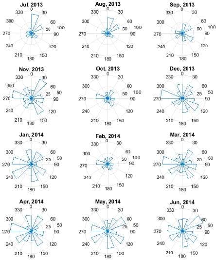
The wind speed (m/h) data used to determine the wind potential of Meşelik Region of Eskişehir with Weibull distribution have been gathered (m/h) in 10-minute intervals through measuring devices installed 10 meters above the ground in Meşelik Campus of Eskişehir Osmangazi University. In the data measurement station, wind blowing directions are also determined via wind direction monitoring device installed 27 meters above the ground. As it is commonly used in wind energy studies, sectors are created as 30-degree slices, and a wind rose graph has been presented in Figure 2 in which wind blowing percentages from each sector are shown graphically.
Figure 2: Monthly wind directions and wind rose graphs of frequencies
Examining Figure 2; it is observed that powerful wind directions vary according to the months of the year. In July and August, the most powerful wind direction is north while in September, it is South-East. While the most powerful wind direction in October, December, February, March, April, and June is west, it is South-West in January.
In the analysis of the wind potential of Meşelik Region of Eskişehir with Weibull distribution, MLE has been obtained by sticking to the results of distribution parameters simulation. RMSE and 𝑅2 performance values have
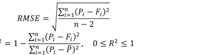
been presented in Table 3 in order to evaluate the fit between parameter estimations obtained by the modeling of monthly wind speeds according to two-parameter Weibull distribution, wind characteristics based on observation, wind characteristics based on parameter Weibull distribution, and the modeling of wind speeds with two-parameter Weibull distribution. Performance measures, RMSE and 𝑅2, which show the fit between the Weibull
Optimum Method for Determining Weibull Distribution Parameters Used in Wind Energy Estimation 645 𝑅𝑀𝑆𝐸 = √∑ (𝑃𝑖− 𝐹𝑖) 2 𝑛 𝑖=1 𝑛 − 2 (32) 𝑅2= 1 −∑ (𝑃𝑖− 𝐹𝑖) 2 𝑛 𝑖=1 ∑𝑛𝑖=1(𝑃𝑖− 𝑃̅)2 , 0 ≤ 𝑅2≤ 1 (33)
The term 𝑃𝑖 in the equation shows the empirical cumulative distribution function value and the term 𝐹𝑖 indicates the
cumulative distribution function value according to two-parameter Weibull distribution. The lower RMSE and higher 𝑅2 value indicates a good fit in the modeling.
Table 3: The parameter estimates (with confidence interval), the wind characteristics in terms of actual and two-parameter Weibull distribution model, and the goodness of fitting performance values
Months Scale shape Mean
Std.
Deviation Power Fitting
𝑪̂𝒍𝒐𝒘 𝑪̂ 𝑪̂𝒖𝒑 𝒌̂𝒍𝒐𝒘 𝒌̂ 𝒌̂𝒖𝒑 Act Wbl Act Wbl Act Wbl R2 RMSE Jul 2013 4.06 4.12 4.17 2.28 2.34 2.39 3.65 3.65 1.66 1.66 49.56 49.38 0.996 0.003 Aug 2013 3.61 3.66 3.71 2.23 2.28 2.34 3.24 3.24 1.50 1.50 35.56 35.19 0.997 0.003 Sep 2013 3.25 3.30 3.35 2.06 2.11 2.16 2.93 2.93 1.46 1.46 27.92 27.85 0.998 0.002 Nov 2013 3.29 3.35 3.41 1.72 1.76 1.80 2.98 2.98 1.77 1.75 37.64 35.74 0.997 0.003 Oct 2013 2.76 2.80 2.85 1.83 1.87 1.92 2.49 2.49 1.38 1.38 18.98 19.30 0.999 0.002 Dec 2013 3.15 3.20 3.25 1.95 2.00 2.05 2.84 2.83 1.47 1.48 25.94 26.67 0.997 0.003 Jan 2014 3.14 3.19 3.25 1.77 1.81 1.85 2.84 2.84 1.62 1.62 30.26 29.73 0.997 0.003 Feb 2014 2.96 3.01 3.06 1.85 1.89 1.94 2.67 2.67 1.47 1.47 23.56 23.65 0.999 0.002 Mar 2014 3.55 3.61 3.67 1.87 1.91 1.96 3.20 3.21 1.75 1.74 41.87 40.30 0.998 0.002 Apr 2014 3.29 3.35 3.41 1.75 1.79 1.83 2.98 2.98 1.74 1.72 35.84 34.92 0.998 0.003 May 2014 3.44 3.50 3.56 1.73 1.77 1.81 3.11 3.11 1.84 1.82 42.15 40.43 0.998 0.002 Jun 2014 3.37 3.43 3.48 1.86 1.91 1.95 3.04 3.04 1.67 1.66 35.34 34.54 0.998 0.003 Examining Table 3, very lower RMSE values and higher 𝑅2 values indicates that the fit in the modeling of wind speed with Weibull distribution is quite good. Moreover, the fit between observation-based wind characteristics and characteristics based on parameter estimations of two-parameter Weibull distributions indicates that the modeling is quite successful. LM estimates, R2 and RMSE values of two-parameter Weibull distribution for wind speeds are
given in Table 4 in order to compare the MLE and LM estimates in terms of goodness of fitting performance values. Table 4: LM estimates of two-parameter Weibull distribution and the goodness of fitting performance values
Months 𝑪̂ 𝒌̂ R2 RMSE Jul 2013 4.114 2.356 0.996 0.003 Aug 2013 3.652 2.335 0.997 0.003 Sep 2013 3.303 2.121 0.998 0.002 Nov 2013 3.351 1.816 0.998 0.003 Oct 2013 2.804 1.862 0.999 0.002 Dec 2013 3.205 1.991 0.997 0.003 Jan 2014 3.197 1.850 0.997 0.003 Feb 2014 3.011 1.889 0.999 0.002 Mar 2014 3.611 1.967 0.999 0.002 Apr 2014 3.347 1.809 0.998 0.003 May 2014 3.495 1.800 0.998 0.002 Jun 2014 3.423 1.933 0.998 0.002
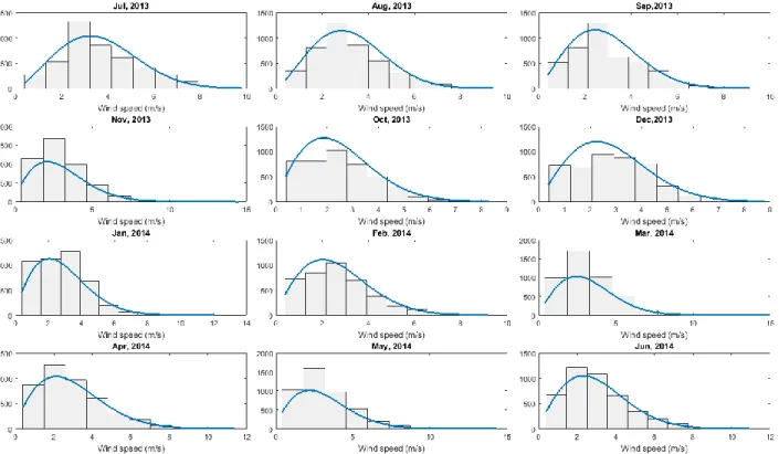
When the goodness of fitting performance values in Table 3 and Table 4 were examined, it was seen that the fit performances of MLE and LM estimates are quite successful and similar. Probability density curves of two-parameter Weibull distribution with histograms of monthly wind speed in Meşelik region of Eskişehir have been given in Figure 3.
Optimum Method for Determining Weibull Distribution Parameters Used in Wind Energy Estimation 646 Figure 3: Wind speed histograms and the probability density curves based on two-parameter Weibull distribution
Examining the mean wind speeds calculated according to two-parameter Weibull distributions in Table 3; the highest mean wind speed is in July with 3.64788 m/h and the lowest mean wind speed is in October with 2.48855 m/h. The concordance between monthly wind speed values observed in Meşelik region of Eskişehir and wind power (W/m2) calculated according to Weibull distribution is presented in Figure 4. In the Meşelik region of Eskişehir, the
highest wind power that could be obtained according to two-parameter Weibull distribution is in July with 49.38295 (W/m2) and the lowest wind power is in October with 19.30044 (W/m2).
Figure 4: Comparison of observed wind power densities with wind power densities calculated based on two-parameter Weibull distribution
Optimum Method for Determining Weibull Distribution Parameters Used in Wind Energy Estimation 647
6. Conclusions
Average wind speed (m/h) data obtained in 10-minute intervals via data measuring devices installed 10 meters above the ground in Meşelik Campus of Eskişehir Osmangazi University are modeled with two-parameter Weibull distribution and the wind energy potential of the region has been statistically analyzed. Six different parameter estimation methods have been compared through a simulation study in order to determine the most suitable estimation method in Weibull distribution parameters estimation. In the comparison of parameter estimation methods, MSE and MAPE criteria have been taken into consideration. As a result of the comparison, LM and MLE have been found as the most successful methods in small and large sample sizes, respectively. In the simulation study, LM has been found as the best alternative parameter estimation method for MLE, which is the most commonly, used method in the modeling of wind speed data with Weibull distribution. The wind energy potential evaluation of the region is performed based on the monthly wind speed (m/h) data. The concordance of the monthly wind speed data of the district in the modeling with two-parameter Weibull distribution has been evaluated based on RMSE and 𝑅2 criteria, and as a result of the evaluation, it has been found as quite good. The fit between wind
characteristics based on observed wind speed (m/h) and wind characteristics based on two-parameter Weibull distribution has also been found as good. In the region, the highest average wind power density has been obtained in July with a value of 49.38295 (W/m2) while the lowest average wind power density has been obtained in October
with a value of 19.30044 (W/m2). Future researches about the estimation of wind potential of Meşelik (Eskişehir)
region could compare wind speeds through devices installed at different heights.
Acknowledgements
The authors gratefully acknowledge Eskişehir Osmangazi University Scientific Research Projects Commission for the financial support of this study through the project number 201015023.
References
1. Akdağ S. A, Güler Ö. (2018). Alternative Moment Method for wind energy potential and turbine energy output estimation. Renewable Energy 2018; 120: 69-77.
2. Ali S., Lee S. M, Jang C. M. (2018). Statistical analysis of wind characteristics using Weibull and Rayleigh distributions in Deokjeok-do Island – Incheon, South Korea. Renewable Energy, 123, 652-663.
3. Aras H. (2003).Wind energy status and its assessment in Turkey. Renewable Energy, 28(14), 2213-2220. 4. Baseer M. A., Meyer J. P., Rehman S., Alam M. M. (2017). Wind power characteristics of seven data collection
sites in Jubail, Saudi Arabia using Weibull parameters. Renewable Energy, 102, 35-49.
5. Carta J. A., Ramírez P, Velázquez S. (2009) A review of wind speed probability distributions used in wind energy analysis. Renewable and Sustainable Energy Reviews, 13(5), 933-955.
6. Erisoglu U., Erisoglu M. (2014). L-Moments Estimations for Mixture of Weibull Distributions. Journal of Data Science, 12, 69-85.
7. Genc A., Erisoglu M., Pekgor A., Oturanc G., Hepbasli A., Ulgen K. (2005). Estimation of Wind Power Potential Using Weibull Distribution. Energy Sources, 27(9), 809-822.
8. Novoa C. H., Pérez I. A., Sánchez M. L., García M. Á., Pardo N., Duque B. F.(2017). Wind speed description and power density in northern Spain. Energy, 138, 967-76.
9. Kantar Y. M., Usta I., Arik I., Yenilmez I. (2018). Wind speed analysis using the Extended Generalized Lindley Distribution. Renewable Energy, 118, 1024-1030.
10. Karakoca A., Erisoglu U., Erisoglu M. (2015). A comparison of the parameter estimation methods for bimodal mixture Weibull distribution with complete data. Journal of Applied Statistics, 42(7), 1472-1489.
11. Marks N. B. (2005). Estimation of Weibull parameters from common percentiles. Journal of Applied Statistics, 32(1), 17-24.
12. Malvaldi, A., Weiss S., Infield D., Browell J., Leahy P., Foley A. M. (2017). A spatial and temporal correlation analysis of aggregate wind power in an ideally interconnected Europe. Wind Energy, 20(8), 1315-1329. 13. Shoaib, M., Siddiqui I., Amir Y.M., Rehman S.U. (2017). Evaluation of wind power potential in Baburband
(Pakistan) using Weibull distribution function. Renewable and Sustainable Energy Reviews, 70, 1343-1351. 14. Soulouknga M. H., Doka S. Y., Revanna N., Djongyang N., Kofane T. C. (2018). Analysis of wind speed data
and wind energy potential in Faya-Largeau, Chad, using Weibull distribution. Renewable Energy, 121, 1-8. 15. Sweeney C., Bessa R. J., Browell J., Pinson P. (2020). The future of forecasting for renewable energy. Wiley
Optimum Method for Determining Weibull Distribution Parameters Used in Wind Energy Estimation 648 16. Teimouri M., Hoseini S. M., Nadarajah S. (2013). Comparison of estimation methods for the Weibull
distribution. Statistics, 47(1), 93-109.
17. Wais P. (2017). Two and three-parameter Weibull distribution in available wind power analysis. Renewable Energy, 103, 15-29.
18. Wang F. K., Keats J. B. (1995). Improved percentile estimation for the two-parameter Weibull distribution. Microelectronics Reliability, 35(6), 883-892.