Selçuk J. Appl. Math. Selçuk Journal of Special Issue. pp. 137-148, 2011 Applied Mathematics
The Determination of Outlier Values by M Estimator in Nonlinear Regression and a Simulation Study
Ahmet Pekgör, A¸sır Genç
Selcuk University, Faculty of Science, Department of Statistics, 42031 Campus, Konya, Turkiye
e-mail: p ekgor@ selcuk.edu.tr, agenc@ selcuk.edu.tr
Abstract. The existence of a few outlier values in the sampling would prevent the information given by the majority of the sampling and all of the statistics would turn to be insignificant. Therefore it is essential to determine the outliers in the sampling. In the literature, there are studies regarding the determination of the outliers in the linear regression. In this study, under the light of the studies of Rousseeuw ve Zomeren (1990) and Wu and Lee (2006), it is aimed to determination of outlier values by M estimator in nonlinear regression, one of the robust location estimators. In the application, the height of a corn plant has been analyzed as the sample data set per weeks in the period of 2008 in the Konya region using the Selçuk STAT statistics package program.
Key words: Nonlinear regression, M estimator, Outlier, Selçuk STAT. 2000 Mathematics Subject Classification: 62J02.
1. Introduction
The existence of a few outlier values in the sampling would prevent the infor-mation given by the majority of the sampling and all of the statistics would turn to be insignificant. That is why the determination of outlier values in a sampling is important. Studies concerning the determination of outlier values in linear regression are available in the literature. Within the perspective of the works of Rousseeuw and Zomeren (1990) and Wu and Lee (2006) for deter-mining the outlier values, this paper aims the determination of outlier values by M estimator in nonlinear regression. The sample data set is the length of a corn vegetable in the Konya region for the year 2008 that is analyzed by Selcuk STAT statistics packet programme for the applications.
One of the significant prerequisites of nonlinear regression is the assumption of normal distribution of mistakes by zero mean and constant variance. In
The Least Squares Method (LSM) is affected by the presence of an outlier in the regression analysis. The reason for this is the equal weight given to all data and the working towards the minimization of the squares of error values if generated. Strong regression estimators are used instead of LSM if error terms are not significantly distributed by the normal distribution or the data includes an outlier (Rousseeuw ve Yohai, 1984).
The presence of more than one outlier in the sample result in that close outliers may sometimes mask themselves. These outliers may even lead to reliable data seen as outlier by classical estimation methods (Rousseeuw ve Zomeren, 1990). 2. Nonlinear Regression and M Estimators
The relation between variables in nonlinear regression is as the nonlinear func-tion of at least one parameter. Consider Y as explained variable vector, X = (x1, x2, ..., xn)T as explaining variables matrix, k explaining variable number
and xi= (xi1, xi2, ..., xik)T , i = 1, 2, ..., n as observation values then nonlinear
regression model will be written as follows
(1) yi= f (xi; θ) + εi, i = 1, 2, ..., n
θ = (θ1, θ2, ..., θp)0 (θ ∈ Θ ⊂ Rp) is stated as an unknown parameter vector
and f , as at least one of the nonlinear function of θ unknown parameter vector elements (Gallant 1975).
M estimators correspond to Maximum Likelihood types of estimators. M estima-tors are generalizing the opinion of location parameter’s Maximum Likelihood estimators in a specified distribution (Huber, 1981).
M estimators minimize the error functions that are more general than absolute error totals or error squares totals. In order to decrease the sensitivity of least square estimators to outliers, M estimators uses a symmetric function of errors the ρ function.
Accordingly, the estimator minimizing the error functions total as given below is defined as M estimators (Huber, 1981).
min θ n X i=1 ρ (yi− f(xi; θ))
The ρ(.) function used here has the following properties: 1. Does not decrease between [0,∞)
2. Even function 3. Continuous 4. ρ(0) = 0
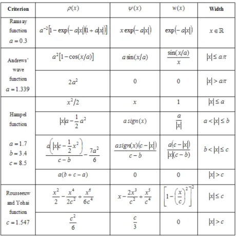
The most widely known ρ(.) function is the Huber function given below that results from the combination of error squares and error absolute values functions.
ρ(x) = ½ x2 2 , |x| ≤ t |x| t −1 2t 2 , |x| > t
The error term t in Huber’s ρ(x) function is taken as t ∼= 2 where the errors were distributed normal (Pekgör 2010).
Given function ψ as the derivative function of function ρ and F (θ) as function f (x; θ)’s parameters according to n×p derivative (Jacobean) matrix, the normal equation system in nonlinear regression, given εi= yi− f(xi; θ) is derived as
(2) F0(θ) ψ(ε) = 0
In order to get the invariant property in equation (2),
(3) F0(θ) ψ³ ε
ˆ σ ´
= 0
is used (Huber 1981). The value of ˆσ used in equation (3) is sound scale para-meter and is calculated as
(4) σ = 1.4826 × MADˆ
The Median Absolute Deviation (MAD) in equation (4) is the median of absolute deviations. This value is calculated widely as,
M AD = medyan {|εi− ε0.5|} , i = 1, 2, ..., n
Here εi is the error value of the i. observation and ε0.5 is the median value
of errors. The constant 1/Φ−1 = 1.4826 in equation (4) makes ˆσ, an unbiased estimator of σ if n is sufficiently big and the error distribution is a normal distribution. When εs
i = εi/ˆσ and where W given as
wii= ψ (εs i) εs i i = 1, 2, ..., n
are the diagonal members of an n × n size diagonal matrix, equation (3) can be written as below (Pekgör 2010).
(5) F0(θ) W (εs) = 0
For W weighted matrix, it can be made different calculations concerning ρ functions and equation (5) can be solved by repeating methods. The most widely used ρ(.) functions used in M estimators are given in Table 1.
Table 1. Some criterion functions in literature
3. The Determination of Outliers by M Estimator
The determination of outliers will be examined in this section under the per-spectives of the works of Wu and Lee (2006) and Rousseeuw and Zomeren (1990) respectively.
3.1. The Determination of the Number of Outlier Values
Wu and Lee (2006) determined the biggest number of outlier observations in a sample under the normality assumption by LAD solution. According to the method named as Outlier Value Number (OVN), m is the biggest number of outliers in a given sample having a N (μ + λσ, σ2) , λ > 0 distribution, and
n −m observations are assumed to have a N(μ, σ2) distribution. In the works of
Agostino and Stephens (1986), experimental normal distribution function can be calculated by equation (6).
(6) F (X; μ, σ) ∼ˆ = i − c
The c values in equation (6) is mostly taken in the literature as c = 0, 0.3, 13, 0.5 and i corresponds to i = 1, 2, ..., n − m. Then ˆUc(xi) values are calculated as
follows:
ˆ Uc(xi) =
x(i)− μ
σ , −∞ < μ < ∞ , σ > 0
Where i is taken as i = n − m + 1, n − m + 2, ..., n the values for ˆUc(xi) are
calculated as follows: ˆ Uc(xi) =
x(i)− (μ + λσ)
σ , −∞ < μ < ∞ , σ, λ > 0
In nonlinear regression the residuals derived by M estimator are used respec-tively for m = 0, (7) Q1(θ) = " n X i=1 ρ µ ˆ Uc(xi) − ei− μ σ ¶# and for m = 1, 2, ...,££n2¤¤ , (8) Q2(θ) = nX−m i=1 ρ µ ˆ Uc(xi) − ei− μ σ ¶ + n X i=n−m+1 ρ µ ˆ Uc(xi) − ei− (μ + λσ) σ 
After estimating μ , σ ve λ values minimizing functions (7) and (8) SMAD sample mean absolute deviation values are calculated for m = 0
(9) SM AD = 1 n − 2 " n X i=1 ρ µ ˆ Uc(xi) − ei− μ σ ¶#
and for m = 1, 2, ...,££n2¤¤ (Pekgör 2010).
A = nX−m i=1 ρ µ ˆ Uc(xi) − ei− μ σ ¶ B = n X i=n−m+1 ρ µ ˆ Uc(xi) − ei− (μ + λσ) σ ¶ (10) SM AD = 1 n − 3[A+B]
Among all c values, the m value having the smallest SMAD value will give the possible biggest outlier number (Wu and Lee 2006).
3.2. Robust Distance Method
For determining multiple outlier observations Rousseeuw and Zomeren (1990) presented their ideas of calculating location and scale parameters used by Mini-mum Volume Ellipsoid method using strong estimators in their works. Accord-ingly, instead of using classical mahalanobis distance in the calculations of an estimator and derived residuals, the usage of equation (11) has been observed leading to stronger results (Rousseeuw and Zomeren 1990).
(11) RDi =
ei− e0.5
ˆ σ
Equation (11) is named as Robust Distance (RD). The square of Maha-lanobis distance has a distribution of chi-square; hence observations satisfying the RD2
i > χ2p,1−α/2rule are regarded as outlier values (Rousseeuw ve Zomeren
1990).
4. Analysis of Observation Effects
Observations further away from other values in the sample, but being above the regression line passing within are considered as good effective values. These observations have very important effects upon model statistics like correlations coefficients and coefficients standard errors. Point B in figure 1 is a good effective value.
Within space Y but outlier observations in space X are named as bad effective values or horizontal outlier values. These observations have crucial effects upon model coefficients and do have pulling effects of the regression line towards themselves. Point C in figure 1 is a horizontal outlier value.
Values away from space Y but being observed normal in space X are named as outlier value in space Y or vertical outlier value. These observations have big residual values. Point A in figure 1 is a vertical outlier value.
Figure 1. Good effective value, vertical outlier value, bad effective value.
5. Application
This section will compare suitable data sets of the scenarios in Figure 2 in Richard’s sigmoidal models
(12) f (x; θ) = θ1
(1 + exp(θ2− θ3x))1/θ4
with OVN and RD methods outlier value determinations in a nonlinear regres-sion model. Monte Carlo simulation Works are carried out by using Selçuk STAT statistics package programme. The programme used the visual pro-gramming language Delphi.
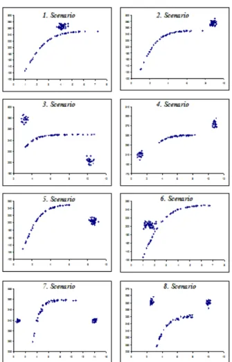
The simulation works carried out will be done for each scenario in Figure 2 with respect to observation numbers 20, 40 and 100 with broken data sets of 10 % and 25 % for each of the 48 situations. The trial number for each situation will be 10.000 (Pekgör 2010).
Figure 2. The scatter graphics of observations derived from scenarios of a simulation
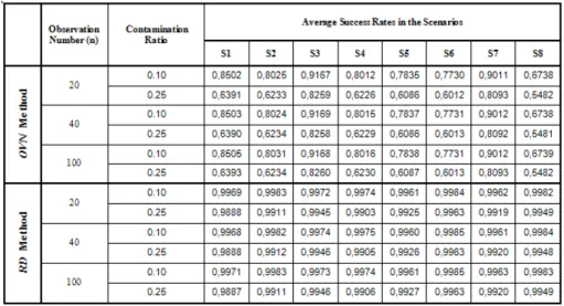
After undertaking the simulation, average success rates in the scenarios gener-ated by the OVN and RD methods are presented in Table 2. Analysing both of the results will show that success rates are better in the RD method than the OVN method.
Table 2. The average success rates of OVN and RD methods in the scenarios
The length of a corn vegetable in the Konya region in the year 2008 according to weeks will be used as sample data set. The scatter graphic for the sample data set is given in Figure 3.
Table 3. Calculated parameter values by OVN method with Huber’s M residuals
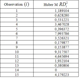
Table 4. Distances of Huber’s M residuals calculated by RD method
After analysing the results in Table 3 and Table 4, the OVN method displays one outlier value in the given data set whereas the RD method shows the non existence of an outlier value since table 4 does not have a value greater than table value of χ2
4,0.975= 11.143.
6. Conclusion and Suggestions
In the simulation works of Richard’s sigmoidal models regarding the determi-nation of outlier observations, the RD method suggested by Rousseeuw and Zomeren (1990) has achieved better results in determining outlier values than the OVN method suggested by Wu and Lee (2006). The scenarios regarding the contamination data are entirely simulations; different scenarios can be produced according to the regression model and the real data set. In the upcoming studies the comparison of other estimators besides M estimator may be undertaken. 7. Acknowledgements
This study is a part of Philosophy of Doctora (Ph.D.) Thesis titled “Compu-tation of Breakdown Points in Nonlinear Regregression and an Application”, Ahmet PEKGÖR, submitted by Selcuk University, Graduate School of Natural and Applied Sciences, Department of Mathematics, Konya, Turkey, 2010. References
2. Gallant, A. R. (1975), Nonlinear Regression, Journal of the American Statistical Association, 29, 73-81.
3. Hadi, A., and Simonoff, J. (1993), Procedures for the Identification of Multiple Outliers in Linear Models, Journal of the American Statistical Association, 88, 1264-1272.
4. Hampel, F. R. (1973), Robust Estimation: A Condensed Partial Survey, Z. Wahrschein-lichkeitstheorie Verw. Gebiete 27, 87-104.
5. Huber, P. J. (1981), Robust Statistics, John Willey&Sons, Inc., USA.
6. Laurent, R. T. S. and Cook, R. D. (1992), Leverage and Superleverage in Nonlin-ear Regression, American Statistical Association Journal of the American Statistical Association, vol. 87, no. 420, pp. 985-990.
7. Pekgör A. (2010), Computation of Breakdown Points in Nonlinear Regregression and an Application, Selcuk University, Graduate School of Natural and Applied Sci-ences, Philosophy of Doctora, Konya.
8. Rousseeuw, P. J. and Yohai, V. J. (1984), Robust Regression by Means of S-Estimator in Robust and Nonlinear Time Series Analysis, eds. J. Franke, W. Hardle and R. D. Martin, (Lecture Notes in Statistics), Springer - Verlag, New York, pp. 256-272.
9. Rousseeuw, P. J. and Zomeren, B. C. (1990), Unmasking Multivariate Outliers and Leverage Points, Journal of the American Statistical Association, vol. 85, no. 411, 633-639.
10. Wu, J. W. and Lee, W.C. (2006), Computational Algorithm of Least Absolute Deviation Method for Determining Number of Outliers Under Normality, Applied Mathematics and Computation, vol. 175, pp. 609-617.