A memetic algorithm for hybrid flow-shop scheduling with multiprocessor tasks and due windows

(1)

T.C.

SELÇUK UNIVERSITY

GRADUATE SCHOOL OF NATURAL SCIENCES

A MEMETIC ALGORITHM FOR HYBRID FLOW-SHOP SCHEDULING WITH MULTIPROCESSOR TASKS AND DUE

WINDOWS

Batuhan Eren ENGİN

Master Thesis

Industrial Engineering Department

January - 2016 KONYA

(2)

Batuhan Eren ENGİN tarafından hazırlanan “A MEMETIC ALGORITHM FOR HYBRID FLOW-SHOP SCHEDULING WITH MULTIPROCESSOR TASKS AND DUE WINDOWS” adlı tez çalışması …/…/…... tarihinde aşağıdaki jüri üyeleri tarafından oy birliği / oy çokluğu ile Selçuk Üniversitesi Fen Bilimleri Enstitüsü Endüstri Mühendisliği Anabilim Dalı’nda YÜKSEK LİSANS TEZİ olarak kabul edilmiştir.

Jüri Üyeleri İmza

Başkan

Prof. Dr. Mehmet AKTAN ………..

Danışman

Prof. Dr. Orhan ENGİN ………..

Üye

Yrd. Doç. Dr. Alper DÖYEN ………..

Yukarıdaki sonucu onaylarım.

Prof. Dr. Aşır GENÇ FBE Müdürü

(3)

TEZ BİLDİRİMİ

Bu tezdeki bütün bilgilerin etik davranış ve akademik kurallar çerçevesinde elde edildiğini ve tez yazım kurallarına uygun olarak hazırlanan bu çalışmada bana ait olmayan her türlü ifade ve bilginin kaynağına eksiksiz atıf yapıldığını bildiririm.

DECLARATION PAGE

I hereby declare that all information in this document has been obtained and presented in accordance with academic rules and ethical conduct. I also declare that, as required by these rules and conduct, I have fully cited and referenced all materials and results that are not original to this work.

Batuhan Eren ENGİN Tarih: 25/01/2016

(4)

iv

ÖZET

YÜKSEK LİSANS TEZİ

ZAMAN PENCERELİ ÇOK İŞLEMCİLİ HİBRİT AKIŞ TİPİ ÇİZELGELEME PROBLEMİNİN MEMETİK ALGORİTMA İLE ÇÖZÜMÜ

Selçuk Üniversitesi Fen Bilimleri Enstitüsü Endüstri Mühendisliği Anabilim Dalı

Danışman: Prof. Dr. Orhan ENGİN

2016, 46 Sayfa

Jüri

Prof. Dr. Mehmet AKTAN Prof. Dr. Orhan ENGİN Yrd. Doç. Dr. Alper DÖYEN

Esnek Akış Tipi çizelgeleme problemlerinin herhangi bir aşamada işlerin birden çok işlemcide aynı anda işlenmesine imkan sağlayan yapıya genişletilmesi yeni bir araştırma konusu sunmuştur. NP-Zor olan Çok işlemcili esnek akış tipi çizelgeleme problemi (ÇİEAÇ) k-aşamalı akış tipi üretimde işlenmesi gereken n adet işten ( ∈ {1,2, … , }) oluşmaktadır. Her bir aşamada mi özdeş paralel makinenin bulunduğu ve i. işin

j. aşamada, sizeij değişkeniyle belirtilen sayıda işlemciye gereksinim duyduğu ve aynı anda işlendiği bir iş çizelgeleme problemidir. Bu çalışmada, ÇİEAÇ probleminin çözümü için Memetik algoritma geliştirilmiş ve en iyi parametre seçimi için deney tasarımı yapılmıştır. Ayrıca, ÇİEAÇ problemine işlerin ortak teslimat süresine sahip olduğu özellik de eklenerek, daha önce literatürde bulunmayan bir problem türü (Zaman pencereli çok işlemcili esnek akış tipi çizelgeleme - ZSÇİEAÇ) geliştirilmiştir. ZSÇİEAÇ problemi çözümünde amaç fonksiyonu, işlerin tamamlanma sürelerine göre erken/geç tamamlanma durumunda ortaya çıkan ceza fonksiyonu olarak alınmış ve problem sonuçları literatüre kazandırılmıştır.

Anahtar Kelimeler: Esnek Akış tipi çizelgeleme problemi, Çok işlemcili, Zaman Penceresi, Memetik

(5)

v

ABSTRACT

MS THESIS

A MEMETIC ALGORITHM FOR HYBRID FLOW-SHOP SCHEDULING WITH MULTIPROCESSOR TASKS AND DUE WINDOWS

THE GRADUATE SCHOOL OF NATURAL AND APPLIED SCIENCE OF SELCUK UNIVERSITY

THE DEGREE OF MASTER OF SCIENCE IN INDUSTRIAL ENGINEERING

Advisor: Prof. Dr. Orhan ENGİN

2016, 46 Pages

Jury

Prof. Dr. Mehmet AKTAN Prof. Dr. Orhan ENGİN Assoc. Prof. Alper DÖYEN

Coupling Hybrid Flow Shop (HFS) with multiprocessor task (HFSMT) brought out a new challenging research topic that drew attention among the researchers recently. HFSMT, which is known to be NP-Hard, contains a set of n jobs ( ∈ {1,2, … , }) to be processed on k-stage flow shop. There are mi identical parallel processors at each stage and the number of processor that job i requires at stage j is denoted by sizeij. Memetic algorithm in which a global search algorithm is accompanied with local search

mechanism is developed to solve HFSMT along with experimental design to determine the best parameter set for each problem set. Also, HFSMT extended by adding a common due window to the problem in which the total penalty incurred by earliness and tardiness of jobs is to be minimized are presented for the first time with this study.

Keywords: Hybrid flow shop scheduling problem, multiprocessor task, time window, Memetic

(6)

vi TABLE OF CONTENTS TEZ BİLDİRİMİ ... iii ÖZET ... iv ABSTRACT ...v ABBREVIATIONS ... vii 1. INTRODUCTION ...1 2.LITERATURE REVIEW ...3

2.1. Literature Survey on HFS and HFSMT ...3

3.MATERIAL and METHOD ...8

3.1. Mathematical Models of FS, HFS, HFSMT and HFSMTDW ...8

3.2. Memetic Algorithm and its Implementation ... 14

3.3. General Structure of Developed Memetic Algorithm ... 23

3.4. Introducing Common Due Windows ... 24

4.COMPUTATIONAL EXPERIMENTS ... 26 4.1. Lower Bound ... 26 4.2. Design of Experiments ... 27 5.CONCLUSION ... 45 6.REFERENCES ... 47 ÖZGEÇMİŞ ... 50

(7)

vii

ABBREVIATIONS

GA Genetic Algorithm

MA Memetic Algorithm

HGA Hybrid Genetic Algorithm

E-GA Efficient GA

FS Flow Shop

HFS Hybrid Flow Shop

HFSMT Hybrid Flow Shop Problem with Multiprocessor Task

HFSMTDW Hybrid Flow Shop Problem with Multiprocessor Task and Due Window

LS List Scheduling

PS Permutation Scheduling

(8)

1

1. INTRODUCTION

Low-cost manufacturing is vital for the manufacturing companies to be one step ahead of the others in terms of competition. In this scope, determining good and optimal (if possible) job schedules while minimizing the production lead-time needs to be focused on as it can drastically reduce the machine idle time and job waiting time and therefore, minimize the extra costs.

The hybrid flow-shop (HFS) manufacturing system, which can often be found in the production of integrated circuit packaging and printed circuit board fabrication (Linn and Zhang, 1999), berth allocation of container terminal, real-time machine-vision systems, workforce management (Chou, 2013), is evolved from combining the properties of parallel machine and flow-shop manufacturing system to meet the requirements of changing manufacturing environment. Coupling HFS with multiprocessor task (HFSMT) brought out a new challenging research topic that drew attention among the researchers recently.

HFSMT contains a set of n jobs ( ∈ {1,2, … , }) to be processed on k-stage flow shop. There are mi identical parallel processors at stage i, and the expression sizeij

indicates the number of machines the jobs requires at each stage. Each task of job j needs to be processed simultaneously on sizeij out of mi machines for pij units of time.

All processors and jobs are available since time zero. The main objective, as in this study, is to find a schedule S* that minimizes the maximum completion time of all jobs (e.g. minimizing the makespan). The problem can be denoted as

Fk(Pm1,…,Pmk)|sizeij|Cmax using the popular three-field notation for scheduling

problems. The problem can be decomposed into the following two sequential decision problems: determining a permutation of jobs (e.g. a solution containing a schedule) at stage 1, and a decoding method to sequence jobs in subsequent stages.

Although HFS and HFSMT have been attracting considerable attention among the researchers recently, to the best of our knowledge, HFSMT accompanied with a common due window has not been studied yet. Time windows are practically important in real world, as jobs can be completed either too early for them to be delivered to the customers as jobs in lot might still be in production process; or too late which would cause customer dissatisfaction or penalty because of late delivery. To conclude, the main purposes of the study can be listed as below:

(9)

2

 A Memetic algorithm will be developed to solve the problem instances generated by Oğuz et al. (2004) for hybrid flow shop with multiprocessor task type. The performance of MA will be compared to the algorithms developed to solve the same benchmark set.

 A common due window will be introduced to the problem HFSMT.

 The same benchmark problems provided by Oğuz et al. (2004) considering a time window for delivery will be solved by using Memetic algorithm. The efficiency of MA in finding good solutions to HFSTDW will be presented.

(10)

3

2. LITERATURE REVIEW

In this section, studies dealing with HFSMT are given in details including the problem types, methodologies and conclusions. Besides, literature survey is included in subsection on the meta-heuristic algorithm used in this study.

2.1. Literature Survey on HFS and HFSMT

Hybrid flow shop scheduling with multiprocessor task problems shown as NP-Hard (non-deterministic polynomial time hard) by Linn and Zhang (1999) has been drawing attention recently.

Oğuz et al. (2004) proposed the first benchmark problem set of HFSMT problem. They provided computational complexity of the HFSMT and proved that the hybrid flow shop scheduling with multiprocessor task is NP-Hard to solve. They also developed a genetic algorithm to test the performance of heuristic for the HFSMT problem in terms of percentage deviation.

Cheng et al. (2004) dealt with two-stage flowshop scheduling problem focused on minimizing the earliness and tardiness of the jobs by introducing a common due window, for which they proposed a branch and bound algorithm (BAB) and a heuristic to solve. They proved that this problem is NP-Complete and they devised lower bounds for the problems. They demonstrated that branch and bound method they proposed can solve the problem in which there are utmost 15 jobs in 5 minutes, otherwise a heuristic comes forth as the computation times of BAB exceeds almost an hour.

Serifoğlu and Ulusoy (2004) proposed a GA for minimizing the completion time of all the tasks in the last stage for the problem HFSMT. Their GA included Roulette wheel selection, one-point and uniform order-based crossover types and the job exchange-replace mutation operator. The initial population in their proposed GAs is fed with three chromosomes: one found by shortest processing time sequence and one found by longest processing time of completion times at first stage and also one found by shortest total processing time method. They found the optimal solution for small-scale problems of HFSMT by running total enumeration method, i.e. testing each possible solution. Their GA results are compared with improved lower bound; solutions obtained by SPT, LPT and STPT heuristics, optimal solutions for small problems and

(11)

4

estimated optimal values for larger problems. They integrate a two-opt local search heuristic into their GA and stated that adding a LS did not lead to a statistically significant improvement in results obtained.

Oĝuz and Ercan (2005) studied on HFSMT and proposed a Genetic algorithm with preliminary test to determine the best combination of the control parameters. They tested four versions of their algorithm and concluded that the algorithm approaches to lower bound better (e.g. average percentage deviation) when the new crossover operator is used along with insertion mutation operator.

Tseng and Liao (2008) proposed a PSO algorithm for the hybrid flow shop scheduling with multiprocessor tasks that adopts a new encoding scheme, local search procedure and new best velocity equation and neighborhood search mechanism.

Ying and Lin (2009) developed a heuristic for multistage hybrid flowshops (HMHF) including a List scheduling decoding method, in which two local search methods are implemented in the algorithm.

Jouglet et al. (2009) dealt with HFS with multiprocessor task by developing a MA which combines a GA and constraint programming (CP) based branch-and-bound local search engine. Their genetic operators include random initial population, while introducing good solutions found by four different priority rules, binary tournament selection method, New crossover operator (NXO) which is especially designed for HFSMT and insertion mutation type. Their MA adopts the idea of improving an offsprings generated after crossover with the branch-and-bound algorithm using CP with a probability constant. The algorithm adopts an incremental population

replacement strategy in which new quality solutions can be chosen as parents for the

very next iteration to gain benefits from them as soon as possible. Also, if the new individual is to be included in the population, they use binary tournament to select two different chromosomes and replace it with the worst one, which they believe that this method is superior than replacing with the worst individual whenever a new chromosome is added in the population, as it is shown by Goldberg (1989), it may lead to early convergence.

Kahraman et al. (2010) proposed a parallel greedy approach (PGA) which involves two phases; called destruction and construction, to solve multistage hybrid flow shop scheduling problem. They tested their algorithm and compared it to the Genetic algorithm proposed by Oğuz et al. (2004) and concluded that their algorithm

(12)

5

outperforms the other in terms of percentage deviation which is defined by the deviation of solutions from the lower bounds provided by Oğuz et al. (2004).

Engin et al. (2011) also proposed a Genetic algorithm to solve HFSMT including that the performance of the proposed GA relies on the genetic operator choices and parameter optimization, such as initial solution, reproduction, crossover and mutation operators and probabilities. They offered a new crossover operator and parameter sizes are optimized through full factorial design of experiment so that the best parameter combination and operators are achieved. They concluded that their algorithm gives efficient results compared to the studies in Oĝuz and Ercan (2005) and Kahraman et al. (2010).

Wang et al. (2011) deals with HFSMT scheduling problem by introducing a SA algorithm to solve them including three different decoding methods (list scheduling (LS), permutation scheduling (PS) and first-fit (FF) method that they developed) which are used individually to deal with the sequence of jobs for stage i, i > 1,…,k. In LS method, the jobs after a stage are sorted in a non-decreasing order of their completion time at the previous stage and the jobs are scheduled iteratively to the first available sizeij processors. In PS method, the sequence of jobs at each stages is the same. In FF

method that they proposed, job g is selected to be inserted into the available insert section (this section emerges if there is idle-time that the job g can be inserted before another job in its solution) if the conditions stated as following are satisfied: the processing time of the selected job g should not exceed the available insert section (idle time) and the processing time of the selected job g is the shortest among the unassigned jobs. Even so, the authors added that the FF method cannot always guarantee better final objective function value. Therefore, they decided to pick up the solution with minimum makespan (or objective function) among the outputs obtained by three methods as the schedule to be used at next stage.

Chou (2013) dealt with HFSMT problem decomposing it into two sequential decision problems; determining the job sequence at stage 1 and decoding method to reschedule the jobs based on different priority rules. They also emphasized that the decoding method plays a vital role in finding better solutions, and his experiments on decoding methods proved his remark. He developed a decoding method namely cocktail decoding method that can incorporate different priority rules, which is used in combination with particle swam optimization algorithm. Cocktail decoding method that

(13)

6

he developed adopts the following priority rules: shortest processing time, longest processing time, shortest total remaining processing time, largest total remaining processing time, smallest processor requirement, largest processor requirement, smallest occupied capacity, largest occupied capacity, smallest total remaining occupied capacity and largest total remaining occupied capacity. The other decoding methods in literature that he used in the comparison were List scheduling (LS), permutation scheduling (PS), first fit (FF), FF1 and FF2. His experiments on two small test problems with (n=5, 10) jobs from Oĝuz and Ercan (2005), Serifoğlu and Ulusoy (2004) showed that FF, FF1 and Delay give the best results over the others. He came to a conclusion that using more than one decoding method is a better strategy. It is reported that PSO algorithm in the study outperformed the other algorithms such as GA, constraint programming, MA, GA_SU and simulated annealing used in other studies in literature.

Xu et al. (2013) improved a shuffled frog-leaping algorithm for HFSMT. Normally, jobs are re-sequenced in non-decreasing order of their completion times after each stage. They emphasized that “forward scheduling decoding method” that they developed is beneficial to apply to reschedule the jobs to decrease the machine idle time between consecutive operations, since HFSMT requires the jobs to be decoded right after a stage and just before going through the next. Again, Taguchi method is implemented to adjust the best parameter values for the algorithm.

Lahimer et al. (2013), proposed a new discrepancy search called climbing depth-bounded adjacent discrepancy search to deal with HFSMT. They stated that CDADS’s performance is in association with the initial solution, thus they considered and compared four different rules, i.e. shortest processing time, shortest processing requirement, the Energy rule where an energy of a task j at the stage i is calculated by pij x sizeij, and normalized SPT applied at the last stage. For small problems, solutions are

compared to the optimal solutions, while the solutions for larger problems are compared to the lower bounds proposed.

Yu (2014) proposed a new, hybrid metahuristic called “twin particle swarm optimization” multiprocessors flow shop scheduling with sequence dependent setup times which incorporates a local search algorithm; solving the data simulated by himself. The author reported that the TPSO outperforms PSO in solving multiprocessors flow shop scheduling with sequence dependent setup times.

(14)

7

Marichelvam et al. (2014) developed an improved cuckoo search (ICS) metaheuristic algorithm which they believe it is the first time to attempt to use CS in solving real-industrial scheduling problem, e.g. HFS with the objective to minimize makespan. They compared their algorithm to genetic algorithm in Oĝuz and Ercan (2005), simulated annealing (SA) in Wang et al. (2011), ant colony optimization (ACO) in Ying and Lin (2006), particle swarm optimization by Li et al. (2014), CS by Burnwal and Deb (2013) and they reported that ICS outperforms them for some of the random benchmark instances.

Liou and Hsieh (2015) extended the multi-stage flow shop scheduling problem by adding sequence dependent setup and transportation times. They proposed a hybrid algorithm (HA) that combines the particle swarm optimization (PSO) and genetic algorithm for the problem in hand. Numerical results showed that developed HA is superior to the PSO and GA for multi-stage flow shop group scheduling problem.

To the best of our knowledge, literature survey revealed that a common due windows assigned to jobs in HFSMT has not been investigated yet. For this reason, in this study it is intended to generate problem instances for HFSMT with due windows and solve it optimally, if possible. Otherwise, near optimal solutions will be obtained by a Memetic algorithm.

(15)

8

3. MATERIAL and METHOD

3.1. Mathematical Models of FS, HFS, HFSMT and HFSMTDW

In this section, mathematical models of “Flow shop”, “Hybrid flow shop” and “Hybrid flow shop with multiprocessor task” and “Hybrid flow shop with multiprocessor task and due window” are given.

3.1.1. Classical Flow Shop Scheduling Problem and Formulation

Classical flow shop (FSSP) is the scheduling problem in which a set of n jobs needs to be operated on a set of m machines with the same given processing order. Basic properties of HFS can be listed as below:

 Each job comprises a set of m tasks.

 There are no precedence constrains among the operations of jobs.  Preemption is not allowed.

 Jobs can only be operated on single machine and each machine can only process single operation at a time.

 The objective functions are generally minimizing the makespan, mean flow time, completion time variance and total tardiness.

 It is usually solved by approximation or heuristic methods as it is proved to be NP-Complete.

Mathematical Model of Flow Shop Scheduling Problem

 Consider three finite sets J, M, O where  J is a set of jobs 1…n,

 M is a set of machines 1…m and  O is a set of operations 1…m.

(16)

9 Denote the followings:

 Ji the i-th job in the permutation of jobs

 Pik processing time of the job Ji ∈J on machine k.

 (∀i∈J) (∀k∈M): vik = waiting time (idle time) on machine k before the start of

the job Ji

 (∀i∈J) (∀k∈M): wik = waiting time (idle time) of the job Ji after finishing

processing on machine k, while waiting for machine k+1 to become free.

The mixed integer programming formulation of FS is as follows, provided by Šeda (2008): ∀i, j ∈ J: _, = 1, 0, ℎ (3.1) ∀i ∈ J: = 1 (3.2) ∀j ∈ J: = 1 (3.3) ∀k ∈ M − {m}: = 0 (3.4) ∀k ∈ M − {1}: = (3.5) (∀i ∈ J − {n}) (∀k ∈ M − {m}): _, + _, + _, = + _, + _, (3.6) = ( + ) (3.7)

In this formulation, Equation (3.2) restricts the jobs to be operated on single machine, Equation (3.3) restricts each machine to process single operation at a time, Equation (3.4) is to assure that waiting time of the first job in schedule to be zero,

(17)

10

Equation (3.5) indicates that the waiting time (idle time) of job 1 on machine k before the start of the operation at machine k, Equation (3.6) specifies the waiting and idle times and Equation (3.7) specifies the makespan.

3.1.2. Hybrid Flow Shop Scheduling Problem

HFS is the flow shop scheduling problem coupled with parallel machine in each stage. The general properties of the HFS are listed below:

 There are single or more machines at each stage ( ≥ 1) and at least one stage must contain more than one machine( > 1).

 Each job has the same flow, though it is not required a job being processed at each stage.

 Jobs can only be operated on single machine and each machine can only process single operation at a time

 There are no precedence constrains among the operations of jobs.  Preemption is not allowed.

 An operation of a job can only be started if its previous operation at previous stage is completed.

 The objective functions are generally minimizing the makespan, mean flow time, completion time variance and total tardiness.

 All jobs and machines are available at time zero.

 It is usually solved by approximation or heuristic methods as it is proved to be NP-Complete.

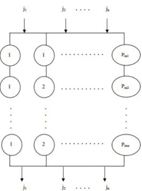
HFS scheduling problem emerges when FS is accompanied with parallel identical machines at each stage. Figure 1-1 depicts the HFS manufacturing type. The formulation below is the work of Lin et al. (2013).

(18)

11

Figure 3-1. Hybrid Flow Shop Scheduling Model, Ceran (2006)

3.1.3. Hybrid Flow Shop Scheduling Problem with Multiprocessor Task

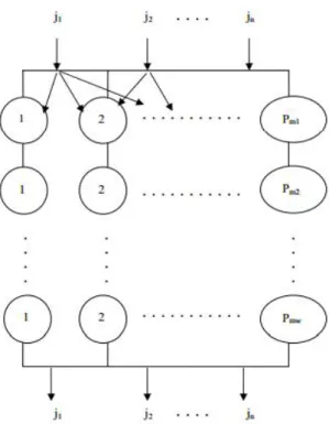
Hybrid flow shop scheduling problem with multiprocessor task (HFSMT) differs from HFS in only one aspect, and that is that a job can be operated on more than a single operator at any stage simultaneously, if necessary. Every assumption made for HFS is still valid for HFSMT.

Figure – 3.2 depicts the Hybrid flow shop scheduling problem with multiprocessor task.

(19)

12

Figure 3-2. Hybrid Flow shop scheduling problem with Multiprocessor Task, Ceran (2006)

Mathematical Model of Hybrid Flow Shop Scheduling Problem with Multiprocessor Task

The following mathematical model is the original work of Lin et al. (2013).

Denote the following variables:  n number of jobs  k number of stages

 mi number of identical parallel machines at stage i

 pij processing time of job j at stage i

 sizeij number of parallel machines required to process job j at stage i

 T planning horizon for which the schedule is to be developed

Let’s denote the following decision variables:

 Xijt a binary time index, which is equal to 1 if job j is processed at stage i in time

period t and equal to 0 otherwise

(20)

13  Cij completion time of job j at stage i

 Cmax makespan

 Let job 0 be the dummy initial job.

The mathematical model can be as follows:

Z=Min Cmax s.t.: ≤ , = 1, . . , , = 1, . . , (3.8) , ≤ , − , = 2, . . , , = 1, . . , (3.9) − + 1 = , = 1, . . , , = 1, . . , (3.10) = , = 1, . . , , = 1, . . , (3.11) ≤ + 1 − , = 1, . . , , = 1, . . , , = 1, . . , (3.12) ≤ + − 1, = 1, . . , , = 1, . . , , = 1, . . , (3.13) ≥ , = 1, . . , (3.14) ∈ {0,1} (3.15) ∈ {1, . . , }, = 1, . . , , = 1, . . , , = 1, . . , (3.16) = 0, = 1, . . , (3.17) ∈ {1, . . , }, = 1, . . , , = 1, . . , , = 1, . . , (3.18)

Constraint (3.8) determines the maximum number of machines at each stage in each time period, Constraint (3.9) restrains a task of job to start before the completion of its’ preceding task. Constraint (3.10) denotes the starting time calculated by processing time requirement, Constraint (3.11) determines the time occupation of each job at each stage. The required number of processors occupation of each job at each stage from starting time until their finishing time are denoted by Constraint (3.12) and Constraint (3.13), respectively. Constraint (3.14) calculates the makespan. Finally, constraints (3.15)–(3.18) define the decision variables.

(21)

14

Mathematical Model of HFSMT with Due Window

This problem is the extension of HFSMT whose mathematical model is given in the previous subsection. Due window are assigned to delivery (completion times of jobs) so that the earliness and tardiness become more of an issue. By adding due window, the objective function becomes the penalty cost function calculated by earliness and tardiness of jobs.

( ) = ( + ) (3.19)

where the expression π represents a schedule and = max 0, − and = max 0, − for a job ∈ , k is the last stage, e and d is the earliest and

latest due date, respectively.

3.2. Memetic Algorithm and its Implementation

Combinatorial optimization problems are frequently encountered in industrial areas such as routing, assignment, job-employee scheduling, network design and other areas of industrial, economic and scientific importance. Methods used to solve these problems are generally classified into three different types, which are exact, approximation and heuristic algorithms. Exact methods guarantee to find optimal solution to the problem in hand, but the computation time significantly increases depending on the problem size. Using heuristics in solving large size problems aims finding good solution in reasonable time. In this study, Memetic algorithm is proposed to solve HFSMT and HFSMT with jobs having a common due window.

Memetic algorithm that has been developed to solve the problem

Fk(Pm1,…,Pmk)|sizeij|Cmax in this study was first addressed in Moscato (1989) and

started to appear in literature in the early 1990s. They defined MAs in their report as the population based heuristics coupled with individual learning and local improvement. It is stated in Ong and Keane (2004) that MAs can balance well between exploration (searching promising areas in search space) and exploitation (searching neighborhoods of individuals in hope of finding better results). It is suggested in Garg (2010) that MAs

(22)

15

are the extension of GAs developed to further improve individual’s fitness in an attempt to reduce premature convergence likelihood. It is also suggested in Burke et al. (1996) that the main benefit of using MAs is the reduction of feasible solution space into subspaces of local optima. They also added that the addition of local improvement methods to genetic algorithm may increase the computational effort but this can be justified with the reduction in search space to reach good solutions.

Memetic algorithms that have been developed and used in literature are generally the extension of Genetic algorithms, which is the case in this study. Therefore, the general steps of GA needs to be included in this section. GAs are the population based metaheuristic algorithm that are based on natural selection concept, aims to evolve the population towards good conditions, selecting parents based on their fitness values to generate offsprings to be included in the next generation through evolutionary operators. In GA, an individual is encoded as chromosome and crossover and mutation are done in this way. Engin (2001) provided the general steps of GA as below:

 Initiate a random generated population,  Encode each individual as chromosome,  Evaluate fitness values of each individual,

 Select parents with selection methods to generate offsprings,

 New offsprings are generated and mutated according to the crossover rate and mutation rate, respectively,

 If new individuals are better in terms of fitness value, the population is updated to include better individuals.

Roulette wheel selection, Tournament selection and Elitism can be shown as selection methods. One point crossover, two point crossover, uniform crossover, three parents crossover can be given as examples to different crossover methods. And one byte mutation, flip bit, boundary, non-uniform, uniform mutation and Gaussian mutation can be given as examples to different mutation methods (Goodman, 2008) .

As mentioned earlier, the difference between MA and GA is the additional local search algorithm applied in MA. It is noticed that some studies in the literature applied local search (LS) procedure only to some of the best individuals; instead of applying to all individuals. Also, several studies applied LS to initial population, some applied it to

(23)

16

the offspring obtained by crossover operator, and some applied it to both the initial population and the offspring. For example, Gao et al. (2011) developed a MA including a local search procedure applied to the first population generated, while Türkbey (2002) developed a MA in which a local search procedure is applied to the first population to search their all neighborhood solutions and also applied to the offsprings generated by crossover operator considering the first neighbor solutions that outperform themselves. Therefore, the stage that LS algorithms are applied at and which solutions that they are applied to are a matter of design that affects the performance of MA.

Memetic algorithm that has been developed in this study consists of Genetic algorithm that causes the population to evolve through four genetic operators; i.e. selection, crossover, mutation and replacement, and local improvement method to further improve the offsprings generated by crossover operator are given in detail below.

3.2.1. Initial Population Generation

Population size parameter determines how many individuals are to be included in the population. The initial population consists of “population size-1” randomly generated individuals. And the population size is kept constant through the generations. One individual is generated by Nawaz, Enscore and Ham (NEH) heuristic published in Nawaz et al. (1983) and fed into the initial generation as an individual to begin search with good initial solution.

The Nawaz, Enscore and Ham Heuristic

NEH heuristic proposed by Nawaz et al. (1983) is known to perform well for the permutation flow shop under the makespan minimization objective. It is based on the idea that the jobs with higher total processing times at each stage on all machines should be scheduled as early as possible to reduce the makespan. The steps into NEH heuristic are given as below:

1. Calculate the total processing times of all jobs at each stage. 2. Sort the jobs in descending order of their total processing times.

(24)

17

3. Take job j, j = 1, . . . , n and find the best schedule by placing it in all the possible jth positions among the sequence of jobs that are already scheduled.

3.2.2. Encoding Scheme

What kind of encoding scheme researchers need to consider are generally driven by the problem type and therefore its nature, i.e. Fk(Pm1,…,Pmk)|sizeij|Cmax in this case.

By definition, HFSMT allows the solver to determine only the sequence of jobs, i.e. the permutation of n jobs, at each stage. Each individual will carry the information of the sequence of jobs.

3.2.3. Decoding Method

Studies in literature dealing with HFSMT differ from each other in either adopting the permutation at first stage for the remaining stages, or decoding the each individual right after a stage to a full schedule by using different algorithms; such as List Scheduling in Oĝuz and Ercan (2005), Lin et al. (2013) which re-sequences the jobs for the stage in non-decreasing order of their completion times at previous stage (first-come-first-served (FCFS)), Permutation scheduling (PS) and first-fit (FF) algorithm in Wang et al. (2011). In this study, List scheduling method is adopted. An example to shed light on how decoding method works is given in this section.

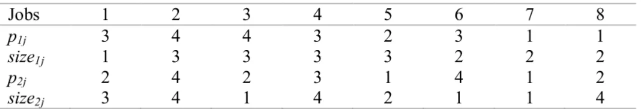
Example: Consider an example with 8 jobs-2 stages and 4 processors at both stages. The processing time and the number of machines required for each jobs are given in Table 1.

Table 3-1. Necessary data for the Example

Jobs 1 2 3 4 5 6 7 8

p1j 3 4 4 3 2 3 1 1

size1j 1 3 3 3 3 2 2 2

p2j 2 4 2 3 1 4 1 2

size2j 3 4 1 4 2 1 1 4

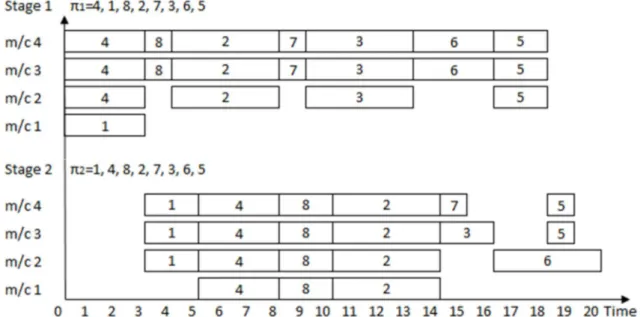
For a given permutation (π1=4, 1, 8, 2, 7, 3, 6, 5) at the stage 1, it is decoded

(25)

18

Figure 3-3. The schedule of the permutation (π1=4, 1, 8, 2, 7, 3, 6, 5) after being decoded by the List scheduling algorithm.

Memetic algorithm operates through the individuals represented by the permutation of jobs at stage 1. List scheduling decodes each individuals into schedules for the remaining stages, i>1, as it can be seen an example in Figure 3-3.

In this example, a semi-active schedule is constructed as follows: jobs from the permutation (π1=4, 1, 8, 2, 7, 3, 6, 5) are iteratively assigned to the processors available

starting from the time 0. We need to pay attention to not assigning a job before its preceding jobs in the permutation, still the jobs can start at the same time if there are enough processors. For example, the job 7 might have started at the same time with the job 8 at stage 1, as there are enough processors for it to be processed. However, this would yield the same results with the permutation of (π*=4, 1, 8, 7, 2, 3, 6, 5), for instance. If this was not the case; it would be very likely to obtain the same solution with different permutations, and this would significantly hamper the Memetic algorithm’s performance as operators such as crossover, mutation or local search cannot make much difference.

3.2.4. Fitness Functions

Individuals compete each other with their fitness values calculated, i.e. makespan, which is the completion time of the last job at the processors at the last stage,

(26)

19

and defined by Cmax. Also, as the due window will be added to the problem later on,

instead of makespan, the cost function Z(π) = ∑ ( + ) will be used for the extended problem with due window.

3.2.5. Selection Method

Individuals from the current population are selected based on their fitness value through the Tournament selection method in order to generate offsprings by crossover operator. Tournament selection method is chosen, as a study in literature showed that Tournament selection method outperforms other selection methods (Noraini and Geraghty, 2011). Steps to Tournament selection are summarized below Goldberg (1989):

1. Define the size of the reproduction pool,

2. Select two individuals from the main population with replacement,

3. Choose the best one from these selected two and keep it in the mating pool, 4. Repeat the Step 1 and 2 until the reproduction pool is full of individuals

selected.

3.2.6. Crossover Methods

Crossover is the main operator that enables the Genetic/Memetic algorithms to search different parts of the solution area by mixing the features of individuals. Parents might produce offsprings or not within the probability called crossover rate (c).

Since mating pool may contain more than two potential parents, in each step, two parents are selected by the same selection method, i.e. Tournament selection, which is used to form the mating pool. Also, since individuals are represented as permutation schedule, crossover operator is carried out considering the fact that a job number cannot be repeated in a chromosome. Different crossover methods coded in order to decide which one gives better outcomes for the problem in hand are listed and detailed as such:

(27)

20 2. Order Crossover

3. New Crossover Operator

Position Based Crossover (PBX)

The position based crossover (PBX) procedure proposed by Syswerda (1989) is summarized in steps as below:

1. Select a subset of positions from the parent A,

2. Genes at these positions are copied to the offspring with the same positions,

3. The other positions are filled with remaining genes with the same relative order as in the parent B.

An example can be seen given to PBX below:

Table 3-2 Position Based Crossover

Parent A 7 1 4 9 0 6 3 2 8 5

Parent B 5 3 4 7 6 8 9 1 0 2 Offspring 5 1 4 9 7 6 3 0 8 2

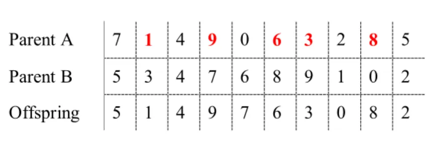
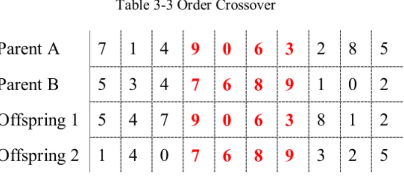
Order Crossover (OX)

The order crossover (OX) procedure proposed by Davis (1985) is summarized in steps as below:

1. Choose a swath consecutive alleles at random from parent A,

2. For offspring 1, copy the swath and fill the blanks with the genes in the same order that they appear in parent B,

3. For offspring 2, copy the swath and fill the blanks with the genes in the same order that they appear in parent A.

(28)

21

An example can be seen given to OX below.

Table 3-3 Order Crossover

Parent A 7 1 4 9 0 6 3 2 8 5 Parent B 5 3 4 7 6 8 9 1 0 2 Offspring 1 5 4 7 9 0 6 3 8 1 2 Offspring 2 1 4 0 7 6 8 9 3 2 5

New Crossover Operator

New crossover operator (NXO) is presented by Oĝuz and Ercan (2005) especially for the HFSMT considering its nature. The insight into the algorithm logic and some example to the implementation of NXO can be seen in Oĝuz and Ercan (2005).

3.2.7. Mutation Operators

Mutation operator is essential to offer the opportunity to escape from trapping the local optima, thus to increase variability and diversity in the population to search different part of the solution area, by mutating genes in chromosomes with several different method from the individuals randomly chosen. A randomly chosen chromosome might be exposed to mutation within the probability called mutation rate (m). The best parameter set for the crossover and mutation rate are determined with experimental design.

Most frequently used mutation operators in literature for the permutation encoding would be “inversion mutation” and “arbitrary three genes” change mutation. The mutation methods are given in steps as follows.

(29)

22

General steps for “inversion mutation” can be given as follows:

1. Choose a random individual to make it exposed to mutation,

2. Select two positions at random, at reverse the sequence between them,

3. Include the mutated individual to the population, regardless of whether it has better or worse value of objective function than its version before the mutation. Example: Assume that a chromosome is given. Let the random chosen numbers (position) be 3 and 7. In this case, the mutated individuals (still Parent 1) would be:

Table 3-4 Inversion Mutation

Arbitrary Three Genes Change Mutation

General steps for “arbitrary three genes change mutation” can be given as follows:

1. Choose a random individual to make it exposed to mutation, 2. Select three positions at random, at exchange their positions,

3. Include the mutated individual to the population, regardless of whether it has better or worse value of objective function than its version before the mutation.

Example: Assume that a chromosome is given. Let the random chosen numbers (position) be 2, 5 and 8. In this case, the mutated individuals (still Parent 1) would be:

Table 3-5 Arbitrary Three Genes Change Mutation

3.2.8. Local Search

Parent 6 3 2 1 9 4 7 5 8 Mutated parent 6 3 7 4 9 1 2 5 8

Parent 6 3 2 1 9 4 7 5 8 Mutated parent 6 9 7 4 5 1 2 3 8

(30)

23

Local search procedure integrated in MA uses the idea of neighborhood that searches the neighbors around the best solution that can be reached within one move, which is a systematic change of jobs position in strings called Insertion. By using Insertion local search applied to the best known solution in an iteration, all schedules obtained by removing a job at the ith position and inserting it in the jth position where i and j is not equal.

3.2.9. Stopping Condition

The algorithm stops searching whether it reaches a certain CPU time spent for each problem, that is 6000 seconds, same with Engin et al. (2011), or if a situation occurs in which the best known solution found so far cannot be improved in 250 consecutive iterations.

3.2.10. Preventing Convergence in Genetic Algorithms

One of the major problems with the use of GA in solving scheduling problems is the chance of premature convergence to local optima. At some point, most of the individuals in population may have the same schedule and objective function, leading to a clone offspring generated in crossover to its parents, therefore cause inefficient search and decrease in quality of the solutions found. To prevent this, we implement the “Random offspring generation (ROG)” before the crossover operation under a certain circumstance. The idea behind the ROG method is that if both parents are the same, instead of generating an individual which would be clone to its parents, a random solution on the problem’s domain is generated. This method is provided by Rocha and Neves (1999).

Also, a reborn strategy is added to the algorithm which ensures that the population is restarted if there is no improvement in the best found solution so far for the predetermined consecutive number of iteration while preserving only the best solution found in the hope of exploration in different solution area.

3.3. General Structure of Developed Memetic Algorithm

(31)

24

 Step 1: Adopt the parameter sizes of GA; such as population size, maximum iteration number, the mutation and crossover rate are determined by full factorial design.

 Step 2: Generate initial population consisting of random individual, including one individual generated by NEH algorithm. Evaluate fitness of each individual in the population.

 Step 3: Check the algorithm stopping criteria. If the condition holds, stop the algorithm and report the best solution and fitness values. Otherwise, proceed to Step 4.

 Step 4: Select parents by using Tournament Selection method (Miller and Goldberg, 1995).

 Step 5: Generate new offsprings with crossover operator and apply mutation procedure to the generated offsprings.

 Step 6: Perform local search using the best known solution.

 Step 7: If the stopping criteria does not hold, go to Step 2. Otherwise, stop the algorithm.

3.4. Introducing Common Due Windows

Time windows are practically important in real world, as jobs can be completed either too early for them to be delivered to the customers as jobs finished and waiting in the inventory may incur inventory cost; or delivered late which would cause customer dissatisfaction or penalty because of late delivery, as stated in the introduction. Therefore, realizing that due windows is an important part of real world situations; it is decided to develop hybrid flow shop scheduling problem with multiprocessor task with the jobs having a common due window.

In order to study on the due dates, there are two approaches. In the first scenario, due dates are given from the customers and asked to meet as much as possible to avoid the penalty cost by scheduling the jobs accordingly. In the other scenario, due dates (whether a common due date valid for all the jobs, or due date set for each job) are determined so that the incurred penalty cost is minimized (Baker, 2014).

As the study by Cheng et al. (2004) sets the due window at the center of Cmax

(32)

25

(0.4*Cmax) (0.6*Cmax), respectively, we adopted the same approach to our problem,

however, we used Cmax found previously in our study. If a job is completed before the

time e, earliness penalty will incur, and if a job is completed after the time d, tardiness penalty will incur, and if a job is completed between the due window, no penalty will incur. The penalty costs calculated for each benchmark instances are given in Table 4-10. As these problem instances extended through a common time window are not solved to optimality yet, we compared the results obtained by MA to GA by removing local search approach from MA. The comparison is given in Table 4-9.

(33)

26

4. COMPUTATIONAL EXPERIMENTS

In this study, the benchmark problem instances that can be found in Oğuz (2006) which consists of 240 problems divided into two types; Type Q and Type P with different combinations of n and k (n=10, 20, 50, 100; k=2,5,8), where each combination contains 10 instances. Although the number of processors at each stage in Type Q are uniformly distributed (U (1, 5)); it is fixed as 5 in Type P problems. This type of problems was proven to be NP-Hard even with 2 stages by Oĝuz and Ercan (2005). Problem names are decoded as “Problem Type_Number of Jobs_Number of Stages_Problem Index”. For example, the problem Q20S5T1 is the first problem in its category (Index=1) and belongs to Type Q problem which is harder to solve than Type P relatively, consisting of 20 jobs and 5 stages. There are 10 instances in each category, in which the number of jobs and the number of stages are the same, therefore 240 instances in hand. The Memetic algorithm is coded in C# language on the Visual Studio 2013 Environment.

4.1. Lower Bound

Lower bounds are calculated by Oğuz et al. (2004) through the formula below:

= max ∈ min∈ + 1 ∈ + min ∈ (4.1)

where j and m denote the set of jobs and stages, respectively, pkj denotes the processing

time of job J at stage k and sizeij denotes the number of parallel machines required to

(34)

27

by MA deviates from the lower bound will be assessed by Percentage Deviation (PD) (Equation 4.2).

( ) = ( ) − ( )

( ) 100 (4.2)

4.2. Design of Experiments

The probability of finding quality solutions with metaheuristics based on genetic operators relies upon the parameter choices, such as crossover rate, mutation rate, population size, iteration size and parent selection rate. Therefore, design of experiment (DOE) is carried out in this thesis. Memetic algorithm executed for different problem sets with different combination of parameters may end up with unlike results. Adopting a parameter set used in GA or MA leading to good solutions does not necessarily yield good results for another GA or MA. Therefore, the Full Factorial design is implemented to decide the best parameter set for each problem type, solving a predetermined problem with each possible parameter combination. Table 4.1 shows the parameter choices.

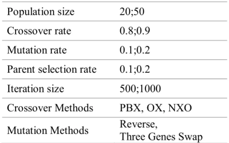
Table 4-1. Parameter Choices used in DOE

Population size 20;50 Crossover rate 0.8;0.9 Mutation rate 0.1;0.2 Parent selection rate 0.1;0.2 Iteration size 500;1000 Crossover Methods PBX, OX, NXO Mutation Methods Reverse,

Three Genes Swap

For each problem category, an instance is chosen out of 10 instances solved by using every possible parameter combinations. For example, for P10S2T01-10 problem type, only P10S2T05 is considered for the design of parameters, and the parameters designed for that problem are generalized for all instances in P10S2T01-10. For this

(35)

28

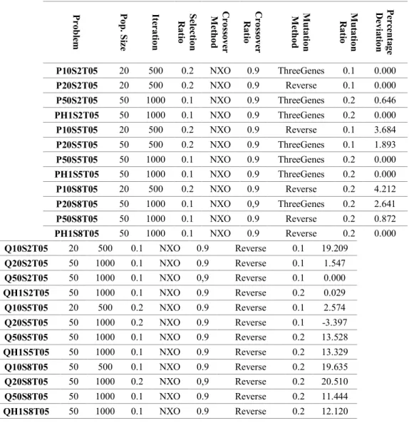
design, 192 (2*2*2*2*2*3*2) separate executions have been made. Table 4-2 shows the parameter choices for each problem category.

Table 4-2. The result of DOE

P r ob le m P op . S iz e It er at ion S e le c ti on R at io C r os sove r M e th od C r os sove r R at io M u tat ion M e th od M u tat ion R at io P e r ce n ta ge D e vi a tion P10S2T05 20 500 0.2 NXO 0.9 ThreeGenes 0.1 0.000 P20S2T05 20 500 0.2 NXO 0.9 Reverse 0.1 0.000 P50S2T05 50 1000 0.1 NXO 0.9 ThreeGenes 0.2 0.646 PH1S2T05 50 1000 0.1 NXO 0.9 ThreeGenes 0.2 0.000 P10S5T05 20 500 0.2 NXO 0.9 Reverse 0.1 3.684 P20S5T05 50 500 0.2 NXO 0.9 ThreeGenes 0.1 1.893 P50S5T05 50 1000 0.1 NXO 0.9 ThreeGenes 0.2 0.000 PH1S5T05 50 1000 0.1 NXO 0.9 ThreeGenes 0.2 0.000 P10S8T05 20 500 0.2 NXO 0.9 Reverse 0.2 4.212 P20S8T05 50 1000 0.1 NXO 0,9 ThreeGenes 0.2 2.641 P50S8T05 50 1000 0.1 NXO 0.9 Reverse 0.2 0.872 PH1S8T05 50 1000 0.1 NXO 0.9 Reverse 0.2 0.000 Q10S2T05 20 500 0.1 NXO 0.9 Reverse 0.1 19.209 Q20S2T05 50 1000 0.1 NXO 0.9 Reverse 0.1 1.547 Q50S2T05 50 1000 0.1 NXO 0,9 Reverse 0.1 0.000 QH1S2T05 50 1000 0.1 NXO 0.9 Reverse 0.2 0.029 Q10S5T05 20 500 0.2 NXO 0.9 Reverse 0.1 2.574 Q20S5T05 50 1000 0.2 NXO 0.9 Reverse 0.1 -3.397 Q50S5T05 50 1000 0.1 NXO 0.9 Reverse 0.2 13.528 QH1S5T05 50 1000 0.1 NXO 0.9 Reverse 0.2 13.329 Q10S8T05 50 500 0.1 NXO 0.9 Reverse 0.2 19.635 Q20S8T05 50 1000 0.2 NXO 0,9 Reverse 0.2 20.510 Q50S8T05 50 1000 0.1 NXO 0.9 Reverse 0.2 11.444 QH1S8T05 50 1000 0.1 NXO 0.9 Reverse 0.2 12.120

Table 4-2 indicates that NXO clearly outperforms the other crossover methods for most of the problem instances. The MA performance is compared to the Genetic algorithm (GA) proposed by Oĝuz and Ercan (2005), Parallel Greedy approach (PGA)

(36)

29

proposed by Kahraman et al. (2010) and Efficient Genetic algorithm (E-GA) approach proposed by Engin et al. (2011). The results are given in Table 4-3 and Table 4-4.

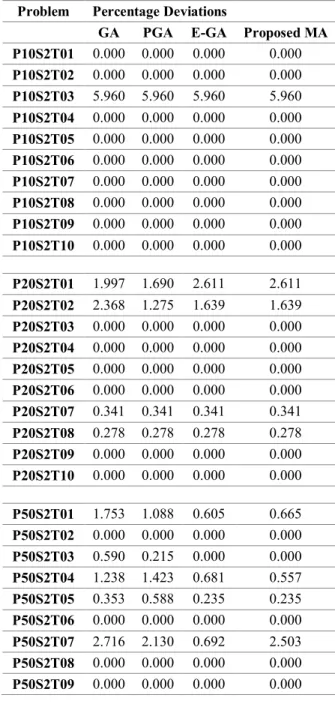
Table 4-3. The obtained results by solving HFSMT with MA and comparison of algorithms

Problem Percentage Deviations

GA PGA E-GA Proposed MA

P10S2T01 0.000 0.000 0.000 0.000 P10S2T02 0.000 0.000 0.000 0.000 P10S2T03 5.960 5.960 5.960 5.960 P10S2T04 0.000 0.000 0.000 0.000 P10S2T05 0.000 0.000 0.000 0.000 P10S2T06 0.000 0.000 0.000 0.000 P10S2T07 0.000 0.000 0.000 0.000 P10S2T08 0.000 0.000 0.000 0.000 P10S2T09 0.000 0.000 0.000 0.000 P10S2T10 0.000 0.000 0.000 0.000 P20S2T01 1.997 1.690 2.611 2.611 P20S2T02 2.368 1.275 1.639 1.639 P20S2T03 0.000 0.000 0.000 0.000 P20S2T04 0.000 0.000 0.000 0.000 P20S2T05 0.000 0.000 0.000 0.000 P20S2T06 0.000 0.000 0.000 0.000 P20S2T07 0.341 0.341 0.341 0.341 P20S2T08 0.278 0.278 0.278 0.278 P20S2T09 0.000 0.000 0.000 0.000 P20S2T10 0.000 0.000 0.000 0.000 P50S2T01 1.753 1.088 0.605 0.665 P50S2T02 0.000 0.000 0.000 0.000 P50S2T03 0.590 0.215 0.000 0.000 P50S2T04 1.238 1.423 0.681 0.557 P50S2T05 0.353 0.588 0.235 0.235 P50S2T06 0.000 0.000 0.000 0.000 P50S2T07 2.716 2.130 0.692 2.503 P50S2T08 0.000 0.000 0.000 0.000 P50S2T09 0.000 0.000 0.000 0.000

(37)

30 P50S2T10 0.262 0.052 0.052 0.052 P1HS2T01 0.534 0.507 0.721 0.107 P1HS2T02 0.000 0.000 0.000 0.000 P1HS2T03 0.814 0.603 0.693 0.814 P1HS2T04 0.000 0.000 0.000 0.000 P1HS2T05 0.000 0.000 0.000 0.000 P1HS2T06 0.000 0.000 0.000 0.000 P1HS2T07 0.926 0.538 0.657 0.837 P1HS2T08 0.020 0.000 0.000 0.000 P1HS2T09 0.105 0.394 0.683 0.499 P1HS2T10 0.097 0.242 0.097 0.000 Table 4-3 Cont’d.

(38)

(39)

Q10S2T01 0.000 0.000 0.000 0.000 Q10S2T02 5.012 5.012 5.012 5.012 Q10S2T03 9.859 0.000 0.000 -23.944 Q10S2T04 0.000 0.000 0.000 0.000 Q10S2T05 0.000 19.209 0.000 19.209 Q10S2T06 5.817 5.817 5.817 6.094 Q10S2T07 0.286 0.286 0.286 0.571 Q10S2T08 12.333 93.33 93.333 93.333 Q10S2T09 4.076 4.076 4.076 6.522 Q10S2T10 7.331 7.331 7.331 7.331 Q20S2T01 7.193 7.193 7.193 7.193 Q20S2T02 0.892 35.414 35.414 35.414 Q20S2T03 4.690 46.529 4.690 46.529 Q20S2T04 0.000 0.000 0.000 0.000 Q20S2T05 0.844 0.703 1.547 1.547 Q20S2T06 0.426 0.426 1.420 0.426 Q20S2T07 0.000 0.000 0.000 0.000 Q20S2T08 0.369 0.369 0.369 0.369 Q20S2T09 0.000 0.000 0.000 0.000 Q20S2T10 1.826 1.674 1.826 1.674 Q50S2T01 0.161 0.161 0.161 0.161 Q50S2T02 0.329 0.329 0.329 0.329 Q50S2T03 1.651 4.068 4.068 4.068 Q50S2T04 0.623 0.187 0.249 0.249 Q50S2T05 0.000 0.000 0.000 0.000 Q50S2T06 2.353 21.799 22.215 21.869 Q50S2T07 0.000 0.000 0.000 0.000 Q50S2T08 3.292 7.081 7.267 7.267

(40)

33 Q50S2T09 2.747 2.816 2.129 2.266 Q50S2T10 2.567 9.949 10.334 10.847 Q1HS2T01 2.250 2.179 2.214 2.286 Q1HS2T02 1.904 1.666 1.360 2.278 Q1HS2T03 3.849 3.952 4.364 3.849 Q1HS2T04 0.000 5.008 0.000 5.756 Q1HS2T05 0.029 0.029 0.029 0.029 Q1HS2T06 0.911 1.058 0.705 2.615 Q1HS2T07 1.891 2.247 1.891 2.110 Q1HS2T08 0.118 0.355 0.118 0.591 Q1HS2T09 1.642 0.000 0.000 -4.580 Q1HS2T10 1.885 1.885 1.778 2.347 Table 4-3 Cont’d.

Q10S5T01 9.291 9.291 9.291 10.135 Q10S5T02 1.536 1.877 2.560 2.560 Q10S5T03 5.664 7.434 9.027 _7.434 Q10S5T04 6.919 14.992 14.827 14.333 Q10S5T05 2.574 2.574 2.574 2.757 Q10S5T06 8.155 10.485 10.485 10.874 Q10S5T07 15.146 15.146 15.146 15.146 Q10S5T08 3.811 0.000 0.000 -18.598 Q10S5T09 0.000 0.000 0.000 -14.732 Q10S5T10 13.163 13.163 13.163 14.145 Q20S5T01 3.533 2.257 2.257 2.257 Q20S5T02 7.970 7.970 7.846 7.846 Q20S5T03 13.626 13.626 12.915 12.915 Q20S5T04 4.277 9.364 9.017 11.445 Q20S5T05 13.907 0.000 0.000 -3.397 Q20S5T06 7.093 10.930 12.093 11.395 Q20S5T07 4.580 4.580 4.580 4.580 Q20S5T08 11.578 11.323 7.761 10.433 Q20S5T09 1.647 3.074 1.207 1.427 Q20S5T10 5.345 5.122 4.120 5.011 Q50S5T01 15.558 13.707 11.163 11.278 Q50S5T02 9.406 7.839 8.567 7.167 Q50S5T03 10.042 0.000 0.000 -2.208 Q50S5T04 11.830 0.100 0.000 -2.607 Q50S5T05 17.784 15.685 13.644 13.528 Q50S5T06 12.231 11.665 9.966 10.702 Q50S5T07 8.294 3.622 1.417 2.205 Q50S5T08 11.680 0.359 0.410 -2.510

(41)

34 Q50S5T09 2.479 0.000 0.000 -8.770 Q50S5T10 2.723 1.733 0.050 -0.198 Q1HS5T01 18.948 10.089 7.813 8.705 Q1HS5T02 15.451 0.000 0.000 -10.335 Q1HS5T03 16.207 2.502 0.227 1.024 Q1HS5T04 18.948 11.750 8.213 8.982 Q1HS5T05 24.866 13.658 10.729 12.971 Q1HS5T06 17.349 7.610 4.855 6.110 Q1HS5T07 24.796 9.139 7.974 7.421 Q1HS5T08 18.322 4.895 2.657 3.105 Q1HS5T09 21.104 3.276 0.443 0.561 Q1HS5T10 22.710 8.952 6.609 6.879 Table 4-3 Cont’d.

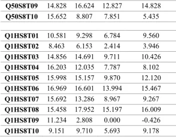
Q10S8T01 15.860 25.134 25.134 26.344 Q10S8T02 7.570 2.789 2.789 2.258 Q10S8T03 8.005 7.349 7.349 6.168 Q10S8T04 2.289 2.169 2.169 4.096 Q10S8T05 19.635 20.700 19.635 21.005 Q10S8T06 13.018 17.456 17.456 18.195 Q10S8T07 14.944 32.432 32.432 31.002 Q10S8T08 13.580 14.938 13.580 16.049 Q10S8T09 18.053 19.937 18.053 20.879 Q10S8T10 7.261 4.331 4.331 5.860 Q20S8T01 11.168 10.656 11.168 10.553 Q20S8T02 18.653 21.634 24.283 21.192 Q20S8T03 10.169 10.829 7.439 9.040 Q20S8T04 9.436 9.347 8.201 5.732 Q20S8T05 18.469 19.898 21.327 19.592 Q20S8T06 11.168 10.143 10.041 9.836 Q20S8T07 40.285 24.808 21.625 21.734 Q20S8T08 21.613 22.366 21.613 19.462 Q20S8T09 20.128 18.522 20.128 20.771 Q20S8T10 14.924 13.909 13.807 13.198 Q50S8T01 20.491 19.151 18.705 20.268 Q50S8T02 14.607 15.236 14.607 13.874 Q50S8T03 9.231 1.921 0.585 0.877 Q50S8T04 24.140 22.742 19.677 18.172 Q50S8T05 22.415 14.016 11.916 11.444 Q50S8T06 13.731 13.068 10.985 13.258 Q50S8T07 9.445 4.035 0.688 0.275 Q50S8T08 24.389 31.505 32.048 31.233

(42)

35 Q50S8T09 14.828 16.624 12.827 14.828 Q50S8T10 15.652 8.807 7.851 5.435 Q1HS8T01 10.581 9.298 6.784 9.560 Q1HS8T02 8.463 6.153 2.414 3.946 Q1HS8T03 14.856 14.691 9.711 10.426 Q1HS8T04 16.203 12.035 7.787 8.102 Q1HS8T05 15.998 15.157 9.870 12.120 Q1HS8T06 16.969 16.601 13.994 15.467 Q1HS8T07 15.692 13.286 8.967 9.267 Q1HS8T08 15.458 17.952 15.197 16.009 Q1HS8T09 11.234 2.808 0.000 -0.426 Q1HS8T10 9.151 9.710 5.693 9.178

The results indicate that the developed MA improved some of the best known solutions so far. For some of the problem instances, the MA reaches the lower bound calculated, or the best known solutions so far.

For 9 out of 10 P10S2T01-10 problem instances the algorithm finds optimal solutions whose objective functions are equal to lower bound. For P10S2T3, the algorithm again finds a solution whose objective function deviates 5.960% from the lower bound.

Figure 4-1. An example to the Iteration Plot graph, a solution of P20S2T02

For 6 out of 10 P20S2T01-10 problem instances the algorithm finds optimal solutions whose objective functions are equal to lower bound. For P10S2T1, P10S2T2,

(43)

36

P10S2T7, P10S2T8 the algorithm again finds solutions whose objective functions deviate 2,611%, 1.639%, %0.341, 0.278% from the lower bound, respectively. The results found for each problem are the same with previous algorithms, except for GA by Oĝuz and Ercan (2005). Figure 4-1 shows that the algorithm may get trapped (resulting same objective function over next generations till the end of the algorithm) in local optima. For this instance, it gets trapped in an optima between the iteration number of 150 and 200, we do not know if it is local or global.

Figure 4-2. Good example of improving objective function over generations

For P50S2T01-10 problem set, for 5 out of 10 problems, MA found solutions whose objective functions are equal to lower bound. For P50S2T01, MA found better solutions than GA and PGA, but worse than Efficient GA. For P50S2T10, MA found a better solution than GA which is equal to Efficient GA and PGA.

For P1HS2T01-10 problem set, for 6 out of 10 problems, MA found solutions whose objective functions are equal to lower bound. For P1HS2T01, MA found a solution that outperforms the others. For P1HS2T07, MA found better solution than GA, but worse than PGA and Efficient GA. For P50S2T09, MA found better solution than Efficient GA, but worse than GA and PGA. For P50S2T10, MA found a solution that equals to lower bound while the others could not.

For P10S5T01-10 problem set, for 1 out of 10 problems, MA found solutions whose objective functions are equal to lower bound. For P10S5T01, MA found a solution better than PGA and equal to GA and Efficient-GA.