Solutions of a 1-D Conservation Laws without Convexity

>

SOLUTION OF A 1-D CONSERVATION LAWS WITHOUT CONVEXITY

Mahir RESULOV and Bahaddin SINSOYSAL

Beykent University, Department of Mathematics and Computing, Ayazaga-Maslak Campus, 34396, Istanbul, Turkey

mresulov@beykent.edu.tr; bsinsoysal@beykent.edu.tr

ABSTRACT

In this paper the exact solution for Cauchy problem of first order nonlinear partial equation with piece-wise initial condition described scalar conservation laws without convexity of the state function. In particular, the state functions having four and one point of inflection are considered. The structure of solutions is investigated.

Keywords: Scalar conservation laws, state function without convexity, convex and concave hull, weak solution

ÖZET

Bu makalede bükeyliği olmayan durum fonksiyonuna sahip birinci mertebeden nonlineer kısmi türevli diferansiyel denklem için yazılmış parçalı sürekli başlangıç koşullu Cauchy probleminin gerçek çözümleri elde edilmiştir. Özel olarak, sırasıyla dört ve bir dönüm noktalarına sahip durum fonksiyonları ele alınmış ve çözümün yapısı incelenmiştir.

Anahtar Kelimeler: Scaler korunum kanunları, bükeyliği olmayan durum fonksiyonu, konveks ve konkav katman, zayıf çözüm.

1. INTRODUCTION

In this study we construct the exact solutions of a scalar conservation law in one dimension as

^ + ^ = 0, x 6 R\ t > 0. (1) dt dx

We assume that the flux function is in C1(R1) and has finite

number of infection points. The equation (1) with the following initial condition

u( x,0) = u0 (x), x 6 R1 (2)

have been investigated in [2], [4]-[7], [11]—[13], when u0(x) 6 Lm(R1). In [3] has been construct fundamental solution of

the equation (1) with initial condition

lim u(x, t) = MS(x), x 6 R1, t > 0, t

where the initial value in distribution sense and M 6 R1 is the total

mass, and S(x) is the Dirac function. It should be noted the problem (1), (2) has been investigated in [1] from practical point of view. In [8]-[11] the method for obtaining the exact solution of this kind problem is proposed.

2. CONSTRUCTION OF THE EXACT SOLUTION

In this section we will construct two problems for different state functions with piecewise constant initial function. As the state function f (u) we consider the functions -C 0 s 2 u and — ,

2 3 respectively.

„ - ^ „ /•/ x cos2u

2.1. The case of f (u) = —-—

In order to find the exact solutions of these problems, according to [4], [12] we formulate the following definitions. We denote by X

the set functions of f defined on [a, fi] which satisfy the inequality f > f (u) .

Definition 1. The function defined by the relation f = inf f (u) is

f 6X called a convex hull on [a, fi] of a function f (u) .

Definition 2. The function defined by the relation f = inf f (u) is

called a concave hull on [a, fi] of a function f (u) .

f 6X

1. At first we will consider the problem (1), (2) for the case

5K 5K

2 4 , 4

.. . cos2u , .

f (u) = on the interval . As it is seen from the Figure 1a) the function 0.5cos2u has four inflection points on the

5k 5k , that is we consider the following equation interval

4 4

du . _ du n

+ sin2u — = 0

dt dx (3)

with the following initial distribution

u0( x )=< - , x <0, 4 - K x >0. 4 (4)

According to Definition 1, we construct the convex hull of the 5K 5K

„ cos2u , , function on the interval

2 4 4 . It is obvious that

K K . u = and u = — are the roots of the equation cos2u = - 1 on

2 2 the interval 5K 5K

4 , 4 . In order to construct the convex hull of

the function - c o s^u , we draw the tangential lines from the points

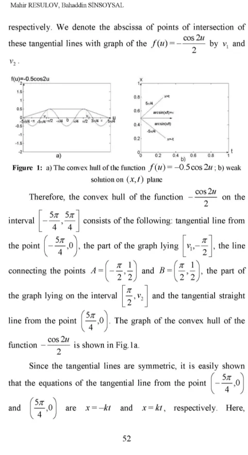
5 K ,0] and f ^ ,0] to the graph of the function ,

respectively. We denote the abscissa of points of intersection of these tangential lines with graph of the f (u) = -cos2u

2 by v and

Figure 1: a) The convex hull of the function f (u) = —0.5cos2u ; b) weak solution on (X, t ) plane

cos 2u

Therefore, the convex hull of the function on the 2

interval 5K 5K

4 ' 4 consists of the following: tangential line from TT

the line ~ * „ ~ L ' 2 J ' f 77- 1 A f 77- 1 A connecting the points A =

( 5 t \

the point ,0 I, the part of the graph lying v 4 J f T 1 , - I and B = v 2 2 J r K (* 1_{— ,— I, the part of} Ï u v 2 2 J

2 , v and the tangential straight the graph lying on the interval

( 5t \

line from the point — ,0 J. The graph of the convex hull of the function — C 0 s 2 u is shown in Fig.1a.

2

Since the tangential lines are symmetric, it is easily shown that the equations of the tangential line from the point 5K

4 0 and — ,0 J are x = —kt and x = kt, respectively. Here, 5k ]

V2 .

r / \

— k = — = sin 2v1. We can not obtain the values of v , V and V1

k naturally, but we may say that v is the least positive root of the

5 t 5 t _{— , v}

2 = v1.

2 2 2 1

equation cot 2 ^ = - 2v, and v1 + v2 =

Since all solutions of the equation (1) are lines having slopes f '(u) and passing through the origin of the (x, t) plane, we

X

convert the function % = — = f '(u) = sin 2u on the interval [—T,0]

1 X

and [0,t]. Solving this equation we find u(x,t) = ——arcsin y and u(x, t) = 1 arcsin X, respectively.

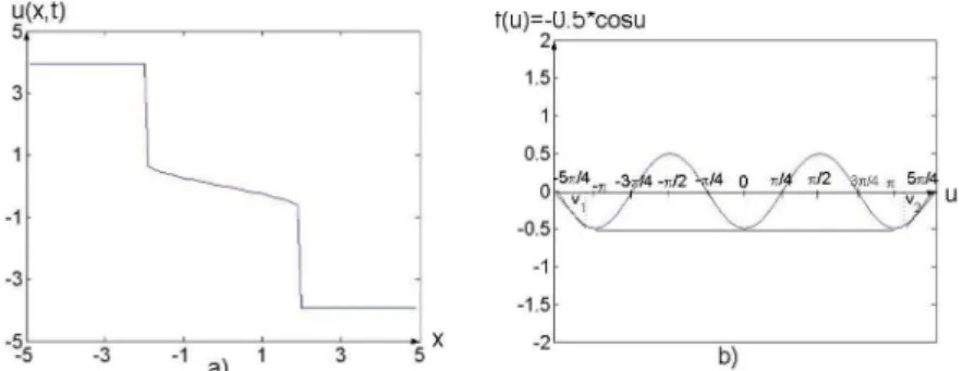
The graph of the weak solution of the problem (3), (4) on the (X,t) plane is illustrated in Fig. 1b. Therefore, the exact solution of the problem (3), (4) is u( x, t ) = < 5 ^ 4 : x < kt, 1 • x — arcsin —, - kt < x < 0, 2 t 1 x — arcsin —, 2 t 4 0 < x < kt, x > kt. (5)

The time evaluation of the solutions of (5) at value T = 1.0 is shown in Fig. 2a.

t(u)=-U.b*cosu

2,

5jt/4 .3 u -jt/2 V 4 0 Tiif */2 \jt/4 n 5JIA x i V ' \ ' / ' \ ' ^i/

Figure 2: a) Time evaluation of the exact solution u ( X, t) a) T = 1 . 0 ; b) The

concave hull of the function f ( u ) = —0.5 c o s 2 u

Now, we investigate the Eq. (3) with the following initial function u0( x ) =< 5K , x <0, 4 5K — , x >0. 4 (6)

In this case we construct the concave hull of the function 5 t 5T

4 ' 4 .. . cos2u , .

f (u) = on the interval

2 . For this aim, we first find the solutions of cos2u = 1, which are u — T and u = T . We denote by A and B the points —

k,—-2 and K,—-2 respectively, and we connect the points A and B by a straight line. We draw the tangential lines from points — ^ ,0 | and

4 J 5k 0 respectively. We also denote the intersections of these tangential lines with the graph f (u) = — °os^u by v and v2, respectively.

cos 2u

Therefore, the concave hull of the function on the interval 5K 5K

4 ' 4

2

consists of the following: tangential line from v

the point 5T

4 ,0 I, the part the graph lying

T

v1s 1 2

f

line connected of the points A = 1

V - T , —2 J I and B =

the straight 1 1 u

T , — I, the 2 J' part of the graph lying on the interval

( I line from the point — ,0 J, Fig. 2b.

T v2,~

2 and the tangential

As above, since the tangential lines are symmetric, their equations are * = - k j and * = k j , respectively. The values of v , v2 and k can not be found, in general, but we may say that v is

, , . . ~ , . , cos2v . _ the least positive root of the equation - k = 1 = sin2vx and

2v

5 t 5 t

V1 + v 2 = y , v 2 = y - V1.

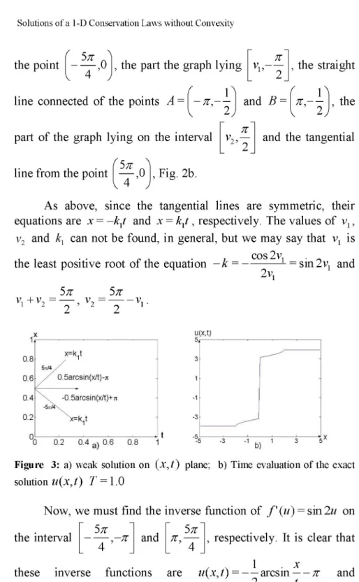
Figure 3: a) weak solution on ( x , t ) plane; b) Time evaluation of the exact

solution u ( x , t ) T = 1.0

Now, we must find the inverse function of f '(u) = sin2u on the interval " 5T " , - T and and ~ 5T T,

_ 4 _ _ 4 _ respectively. It is clear that

these inverse functions are u( x, t ) = - ^ a r c s i nX -% and

2 t . . 1 . x

u(x, t) = — arcsin — + K . 2 t

As a result, the exact solution of this problem is 4 , u( x, t ) = < x < k,t, 1 • x — arcsin K, — kJ < x <0, 2 t 1 (7) 1 . x v 7 — arcsin — + K, 2 t 5K 4 , 0 < x < kt, x > kxt.

The graph of the weak solution of this problem on the (x, t) plane is illustrated in Fig. 3 a. The time evaluation of the solution (7) at T = 1.0 is shown in Fig. 3b.

2.2. The case of f (u) = u

3

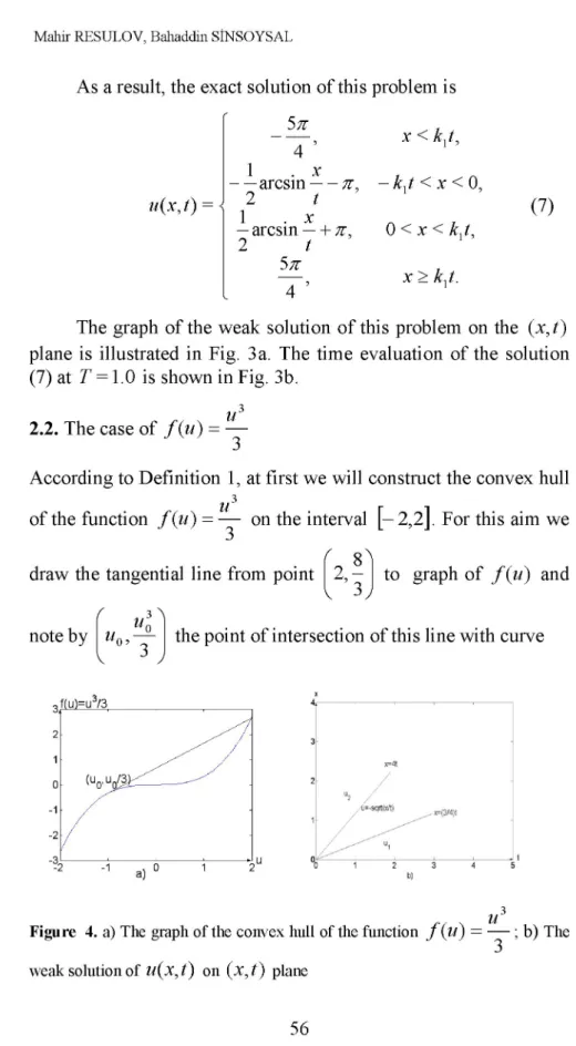
According to Definition 1, at first we will construct the convex hull of the function f (u) = — on the interval [— 2,2]. For this aim we draw the tangential line from point i 2,8 ] _{V 3 J} to graph of f (u) and note by

'

U

KMt U! / u=-sqrt(>Jt) U1 (3/4)1 1 2 3 b)

Figure 4. a) The graph of the convex hull of the function f ( u ) = — ; b) The

weak solution of u(X, t) on (X, t ) plane

— . It is clear that, the value of u0 is found from the relation

3 u

m = f

\

o) =

u Uq

w

Therefore the convex hull of the function — on the interval 3

[ - 2,2] consists of the following: tangential line from the point

( 2, ^ 1 and the part of the graph of lies between point of

( . 1 ] . ( _ 1 ] —1,—

v 3 , and — 2 , — v 8 , , Fig. 4a.

It is clear that the solution is exposed to jump on the line x = Çt, t > 0 which is paralel to the tangential line. From Rankino-Hugoniot condition we have Ç = f ( 2) — f ( 0) = 1. This

u 2 — u 0

jump lies between u0 = —1 (x >Çt) and ^ — H e r e , ^ — | is

inverse function of the Ç = f '(u) = u2 on the interval [— 2,-1].

Hence, u = J - ] = (f')—1 = — x, 1 < £ < 4.

It is clear that intersection of the function ^ — j with line

u2 = - 2 take place on the ray — = 4t. But this ray is paralel to the

tangential line leaving from point ( u 2 , f (u 2)) =

Therefore, the solution of the problem (1), (8) is i 3 A _{u 3}

u, , —

> 3

v 3

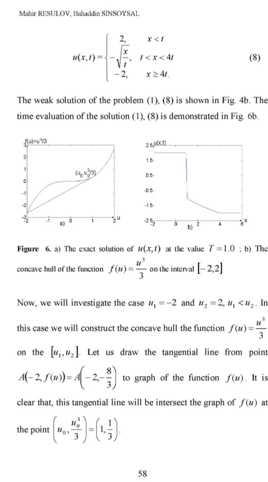
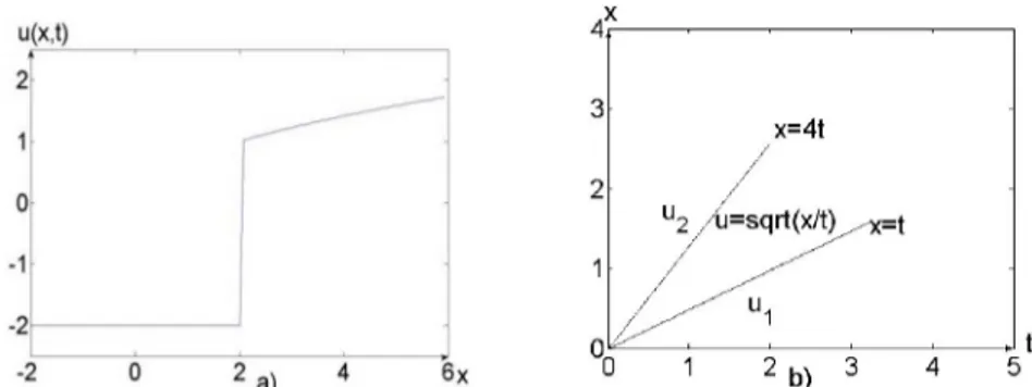
u( x, t ) = < 2, x < t x ^ J , t < x < 4t - 2, x > 4t. (8)

The weak solution of the problem (1), (8) is shown in Fig. 4b. The time evaluation of the solution (1), (8) is demonstrated in Fig. 6b.

Figure 6. a) The exact solution of u ( x , t) at the value T = 1.0 ; b) T h e

concave hull of the function f ( u ) = — on the interval [— 2 , 2 ]

Now, we will investigate the case ux = - 2 and u2 = 2, ux < u2. In

this case we will construct the concave hull the function f (u) = u on the [ u , u2 ]. Let us draw the tangential line from point

A( 2, f (u)) = A 2 ,

-3 to graph of the function f (u) . It is clear that, this tangential line will be intersect the graph of f (u) at

( ,.3 "N the point u„ u 3 ( 1 ^

V,3 y

Figure 7. a) The graph of the function (9); b)The weak solution of the problem

(1), (8) on the (x, t ) plane

u

Therefore, the concave hull of the function f (u) = — on the interval [— 2,2] consists the part of the graph of f (u) lies between points of

3 y and f — 2,—8 j, and tangential line leaving from the 8

point of 2 , - ~ J , Figure 6a. In this case the solution is exposed to jump on the ray x = Çt, t > 0 with is paralel to tangential line

originated from point ( - 2,-8-j. As above, from Rankino-Hugoniot condition we get Ç = 1. This jump take place between

x x

u0 = 2 (for X > t) and J. Here J is inverse function of

£ = f '(u) = u2 on the interval [1,2]. From here we have u = ^ ,

1 4. Therefore the exact solution of the problem (1), (8) (in the case ux < u2) is

u( X, t) = <

- 2, x < t ^y, t < X < 4t

2, x > 4t.

(9)

The graph of the function (9) is shown in Figure 7a. The weak solution of the problem (1), (8) is given Figure 7b.

REFERENCES

[1] Collins, P. Fluids Flow in Porous Materials. 1964.

[2] Goritskii, A.A., Krujkov, S.N., Chechkin, G.A. A First Order Quasi-Linear Equations with Partial Differential Derivatives. Pub. Moskow University, Moskow, 1997.

[3] Kin, Y.J., Lee, Y., Structure of Fundamental Solutions of a Conservation Laws without Convexity, Applied Mathematics, vol.8, pp. 1-20, 2008.

[4] Krushkov, S.N., First Order Quasilinear Equations in Several Independent Variables, Math. USSS Sb., 10, pp.217-243, 1970.

[5] Lax, P.D. The Formation and Decay of Shock Waves, Amer. Math Monthly, 79, pp. 227-241, 1972.

[6] Lax, P.D. Weak Solutions of Nonlinear Hyperbolic Equations and Their Numerical Computations, Comm. of Pure and App. Math, Vol VII, pp 159-193, 1954.

[7] Oleinik, O.A., Discontinuous Solutions of Nonlinear Differential Equations, Usp.Math. Nauk, 12, pp. 3-73, 1957.

[8] Rasulov, M.A. On a Method of Solving the Cauchy Problem for a First Order Nonlinear Equation of Hyperbolic Type with a Smooth Initial Condition, Soviet Math. Dok. 43, No.1, 1991.

[9] Rasulov, M.A., Conservation Laws in a Class of Discontinuous Functions, Seckin, Istanbul, 2011 (in Turkish).

[10] Rasulov, M.A.,.. On a Method of Calculation of the First Phase Saturation During the Process of Displacement of Oil by

Water from Porous Medium. App. Mathematics and Computation, vol. 85, Issue l, pp. l-16, 1997.

[11] Smoller, J.A., Shock Wave and Reaction Diffusion Equations, Springer-Verlag, New York Inc., 1983.

[12] Toro, E.F, Riemann Solvers and Numerical Methods for Fluid Dynamics. Springer-Verlag, Berlin Heidelberg, 1999.

[13] Whitham, G.B. Linear and Nonlinear Waves, Wiley Int., New York, 1974.