Assembly Time Minimization for an Electronic Component Placement
Machine
ALI FUAT ALKAYA
1, EKREM DUMAN
2, AKIF EYLER
31
Computer Science and Engineering Department, Marmara University, 34722, Istanbul, TURKEY
2
Industrial Engineering Department, Dogus University, 34722, Istanbul, TURKEY
3
Industrial Engineering Department, Marmara University, 34722, Istanbul, TURKEY
[email protected], [email protected], [email protected]
Abstract: - In this study, a new algorithm for a particular component placement machine is proposed. Also, a pairwise exchange procedure is designed and applied after the proposed algorithm. In the analyzed machine, previously proposed algorithms were mounting the components from lightest to heaviest where we propose to mount the components from heaviest to lightest. This method brings new opportunities in terms of performance gain on typical Printed Circuit Boards produced in the industry. The new algorithm is compared with former approaches on synthetically generated instances. It outperforms the former approaches by 1.54 percent on printed circuit boards with 100 components to be placed. It gives better results in 96 out of 100 instances. Applying the designed pairwise exchange procedure after the proposed algorithm further improves the total assembly time. Moreover, by taking advantage of inherent design of the analyzed PCBs, other promising improvement procedures are also suggested for minimizing total assembly time. By applying all the suggested techniques to the problem instances, performance improvement rate reaches up to 4.5 percent when compared with previous studies. Since the architecture and working principles of widely used new technology placement machines are very similar to the one analyzed here, the improvement techniques developed here can easily be generalized to them.
Key-Words: - Printed Circuit Board Assembly, Traveling Salesman Problem, Placement Machine
1 Introduction
The use of automated placement machines and optimization issues emerging from them has attracted the interest of researchers for a few decades. Since a small percentage of improvement can bring huge economical benefits, it is still worth to study on them. It is necessary to solve the optimization problems inherent to these machines to get the best performance from them.
Basically, the operations of these machines yield four major problems [1]. These are, allocation of component types to machines, determination of board production sequence, allocation of component types to feeder cells (also called the feeder configuration problem) and determination of component placement sequence. In many other studies, this list is extended or shortened but the last two have great influence and hence importance in optimizing the PCB machines [2,3]. All of these problems are interdependent, that is solution of one affects the other. Depending on the principles of the machine, some may be trivially solved while in most cases they yield NP-Complete problems. Hence a solution aiming to achieve the optimum in all problems simultaneously is very difficult to find,
if not impossible. In this study, we investigate a machine type whose operations involve feeder configuration and placement sequencing problems.
When the placement sequencing problems emerging from these placement machines are examined, it is seen that the problem mostly has a similarity to the well-known Travelling Salesman Problem (TSP). Due to the operations of placement machines the distance between two placement locations is calculated by either Chebyshev or Euclidean distance measure. Different machine designs may lead to different problems and this is observed in the different formulation of the placement sequencing problem where several variants of TSP arise. These variants may be listed as the precedence constrained TSP or multiple TSP [4,5,6]. Currently we are working on a machine structure that may be formulated either the Prize Collecting TSP or the Vehicle Routing Problem (VRP) [7,8]. The referred TSP and its variants are NP-Complete problems and there are good heuristics for solving them [1,9,10,11,12].
Mostly, we can formulate the feeder configuration problem as either an instance of the
Linear Assignment Problem or the Quadratic Assignment Problem [13,14,15,16].
In a previous study, Duman modeled the operations of a component placement machine with rotational turret and stationary component magazine [17]. After modeling the operations of this machine, two problems are formulated; the placement sequencing problem and the feeder configuration problem. In the study, it is shown that the placement sequencing problem can be modeled and solved as a classical TSP whereas the feeder configuration problem is solved in an ideal way by a proposed procedure. The proposed algorithm for the placement sequencing problem is called the Assembly Time Minimization Algorithm (ATMA). The results show that it brings an improvement in terms of total assembly time for this type of machines when compared with the industrial solution used up to that date.
In this study, we propose an improved version of the ATMA algorithm called the inverse ATMA (iATMA) and designed a pairwise exchange procedure for seeking further improvements. This newly proposed procedure outperforms ATMA in terms of total assembly time. Two algorithms are compared on randomly generated PCB data and about 1.75% improvement is gained on the average. In the next section, we give the problem definition and an overview of the working principles of the analyzed machine type. Section 3 gives a summary for ATMA. In Section 4, we give detailed explanation for iATMA, pairwise exchange procedure and further improvement techniques that give promising results. Section 5 gives the details of comparison study and Section 6 includes the summary and conclusions.
2 Machine Working Principles and
Problem Formulation
In the industry, there are two technologies used in the PCB assembly. These are surface mount technology (SMT) and pin-thru insertion technology [18,19]. SMT has gained wide acceptance in the last decade when compared with pin-thru insertion technology. In SMT the components are placed over points pre-covered by an adhesive material. In this study, the machine we investigate is an SMT. The particular machine type investigated is TDK brand, model RX-5A SMD placement machine.
Methodologies proposed for improving the performance of this machine are valuable because, a new, latest technology, widely accepted model of placement machines (called ‘chip shooters’ in the
industry) are also based on the rotating turrets and have similar working principles. Therefore, any improvement obtained for the machine analyzed in this study can also be generalized to chip shooters.
2.1 Working Principles
The machine has a rotational turret which includes 72 heads. These heads take the components from the component magazine and during the rotation of the turret the head reaching the placement location over the board moves down and makes the placement to the precise location on the PCB which is pre-aligned with the placement position by the board carrier actions. The component magazine is stationary, has a circular structure placed behind the machine (Figure 1).
By the time the next head reaches the placement location, the PCB is aligned to the exact position where placement will occur. This alignment is achieved by the simultaneous movements of the board carrier which results in a Chebyshev distance measure. 22 61 1 Feeder Slot 1 Pickup Zone No-Pickup Zone PCB Board Carrier Placement Location Feeder Slot 40 X Y
Figure 1– Diagram of a Placement machine with rotational turret and stationary component magazine
Another important property of the investigated machine is that it can handle component types of different weight. To cope with this each head is equipped with three suction nozzles compatible with different weight categories. When a component of heavier type is picked up by any of the heads, the rotation speed of the turret is reduced. For the machine type that is under analysis, we have four discrete speed values corresponding to four different weight categories. These are 0.20, 0.23, 0.33 and 0.40 seconds per rotational movement of distance one head, ordered from lightest to heaviest components. Even though the machine has actually 72 heads, in the figure we depicted a few for the
sake of clarity. If we label the heads with numbers as illustrated in the figure, with number 1 being the placement head, component tapes on the component magazine stand along the heads from 22 up to 61, forming the pickup zone. What component type should each and every head pick up is known. Then, during the rotational movement of the turret, the head(s) situating over the correct component tape move down and pick a component. The other movable part of the machine, the board carrier, has a speed of 120 mm per second in both x and y directions.
Mechanically, there are two sets of operations that follow each other sequentially and the operations in each set are performed simultaneously. Operations in the first set includes:
i) turret rotates and the next placement head comes over the PCB,
ii) board carrier aligns the new placement point under the placement head,
iii) placement heads rotate if necessary to align the suction nozzle carrying the component to be placed.
In the second set there are:
i) the placement head moves down, makes the placement and moves up,
ii) heads in the pickup zone that are above the appropriate component tapes move down and pick up components.
In [17], a more detailed explanation of the operations of this machine can be found.
2.2 Problem Formulation
Basically, the goal is to optimize the PCB assembly time of the machine considered, but this can be achieved by an efficient solution of the placement sequencing and feeder configuration problems.
When one has a deeper look at the whole problem, he can easily see that what makes it complicated is the varying speed of the turret. In order to see this, for a moment let us relax this constraint/working principle of the machine, i.e. let us assume that the rotational turret has unique speed for all weight categories. Then the rotational turret has a uniform rotational speed throughout the whole assembly process, and the problem turns out to be only a placement sequencing problem, because the feeder configuration problem vanishes. If we let tij
be the time between the completion of consecutive placements at points i and j, then it can be calculated by using the following definitions.
t0 = component placement time (including placement head moving down and up time),
txij = board carrier movement time in x direction
between points i and j,
tyij = board carrier movement time in y direction
between points i and j,
tt = turret time (turret rotation time required for the next placement head to arrive over the PCB),
Then, tij is given by the following expression
{
y t}
ij x ij ijt
t
t
t
t
=
0+
max
,
,
(1) Observe that the formulation turns out to be a TSP with Chebyshev distance measure with the distance between two points is calculated by equation (1).Now, let us take into account the varying speed of the turret according to components. At any time of the assembly process the speed of the turret is determined by considering the heaviest component an all of 60 heads. So, the value of tt, hence total assembly time, depends both on the feeder allocation and placement sequence. This means that the classical TSP formulation given for the PCB assembly time minimization problem cannot be valid anymore since it needs a constant distance between every pair of points. So, we can see that what makes the problem complicated is the varying speed of the turret.
On the other hand, given a placement sequence, the objective of the feeder configuration problem is to find the optimum positioning of the component tapes within the magazine so that, the number of slower steps taken by the turret is minimized.
3 Previous Work (ATMA)
For the problem that originates from the placement machine type under analysis, to the best of our knowledge, the only work belongs to Duman [17]. Therefore the discussion for previous work will cover only this study.
The placement sequencing problem (for a given feeder configuration) should be regarded as the main problem since its solution directly gives the PCB assembly time. Accordingly, Duman regards the feeder configuration problem as the auxiliary problem [17]. The variable and complicated nature of tt not only makes the placement sequencing problem difficult but also makes the TSP formulation infeasible. However, it turns out that, from the placement machine investigated, this change in the tt values makes placement sequences of mixed light and heavy components quite inefficient. Accordingly, it seems to be a good idea to place all of the lighter components first and then the heavier ones. This way, the tt values corresponding to each weight category would be
constant and it would be possible to use the TSP formulation to find the placement sequences within each weight category. This is the idea behind ATMA.
The given solution procedure includes firstly finding TSP routes for each weight category, connecting these routes and then given these placement sequence the optimal feeder configuration is obtained by assigning the component types to the feeder locations in the order of first appearance in the placement sequence. This is known as the Feeder Assignment Procedure (FAP) and is detailed below. The routes are obtained using Convex Hull and Or-Opt algorithms [20].
Algorithm ATMA:
i) Find TSP routes for each weight category. Call the route for weight category 1 as Route 1, and so on.
ii) Connect Route 2 to the last point of Route 1 through the shortest connection. Rearrange Route 2 to make the connection point as the home city.
iii) Repeat Step 2 to connect Route 3 to the modified Route 2 and Route 4 to the modified Route 3.
iv) Apply FAP to find the feeder configuration. v) Recalculate the assembly time using the
modified TSP routes and the tt values found through FAP.
Feeder Assignment Procedure (FAP):
i) Assign sufficient number of slots to each group of components where group 4 takes the closest slots to the PCB, group 3 takes the set of next closest slots, and so on.
ii) For the internal arrangement of each group, assign component types to feeder slots in the order of their first appearance in the placement sequence.
4 Proposed Algorithm (iATMA) and
Further Improvements
In this study, we propose an improved version of the ATMA algorithm called iATMA and obtain further improvements by a random search procedure.
4.1 iATMA
The idea behind iATMA is similar to ATMA in terms of the algorithmic steps. The basic difference that it proposes is in the order of placement of component groups. Both algorithms mount the
components in groups of their weight categories. ATMA places the component groups starting from group 1 to group 4 (i.e. heaviest to lightest), but iATMA inverses this process such that it starts mounting the components from group 4 to group 1 (i.e. lightest to heaviest).
Algorithm iATMA:
i) Find TSP routes for each weight category. Call the route for weight category 1 as Route 1, and so on.
ii) Connect Route 3 to the last point of Route 4 through the shortest connection. Rearrange Route 3 to make the connection point as the home city.
iii) Repeat Step 2 to connect Route 2 to the modified Route 3 and Route 1 to the modified Route 2.
iv) Apply FAP to find the feeder configuration. v) Recalculate the assembly time using the
modified TSP routes and the tt values found through FAP.
We propose no new ideas for FAP because it already gives ideal solutions.
In order to see the improvement that iATMA provides, consider the following example. Let N=100, i.e. 100 components will be assembled with the following weight categories: N1=80, N2=10,
N3=5 and N4=5 where increasing index value
identifies heavier component categories. After configuring the feeder slots as stated in the FAP, using ATMA, it can be found that the number of rotational steps of the turret in each speed category (SCi) as 50, 15, 10 and 25, respectively, if
continuous assembly process of the PCB assembly is considered.
If the iATMA is to be used in this example, the number of rotational steps of the turret in each speed category would be 60, 10, 5 and 25.
If we assume that the x-y movements of the board carrier can be completed within the allowed turret time, tt, then, the sum of the ‘number of placements in a speed category i times the corresponding tt values’ plus N*t0 can be defined as the Lower Bound (LB) for the PCB assembly time. Clearly, the LB values of the algorithms is a comparison criterion. If the various tt values are labeled as tti with higher index showing slower tt
value, then we can define LB mathematically as follows.
∑
=×
+
×
=
n i t i it
SC
t
N
LB
1 0 (2)Comparing the performances of the iATMA and ATMA with respect to LB, we see that for the above example ATMA would populate a PCB in 26.75
seconds while iATMA would populate the same PCB in 25.95 seconds. This gives about a 3% improvement.
In order to trace the steps in the algorithm and movements of the turret, we constructed the following hypothetical small rotational turret system (see Table 1).
Table 1
—
Data forhypothetical small rotational turret systemGroup ni Types of
components Ni
Placement sequence (given) 1 (lightest) 4 X,Y,Z,T 8 X,Y,Z,T,T,Z,Y,X
2 3 P,Q,R 7 P,Q,R,P,Q,R,P
3 3 K,L,M 7 K,K,L,M,L,M,K
4 (heaviest) 3 A,B,C 6 A,B,B,A,C,A
N=28
Say that, the placement sequences are already determined by using the appropriate TSP solving algorithm (Convex-Hull and Or-Opt). As stated before, larger index values stand for heavier component groups. Next, using FAP we assign a sufficient number of slots to each group of components, where group 4 takes the closest slots to the PCB, group 3 takes the set of next closest slots, and so on, and for the internal arrangement of each group we assign component types to feeder slots in the order of their first appearance in the placement sequence. This is illustrated in Figure 2.
No-Pickup zone 1 2 10 9 8 7 6 5 4 3 11 12 13 14 15 16 A B C K L M P Q R X Y Z T Pickup zone Placement Location
Figure 2 – Hypothetical small rotational turret system
In this hypothetical rotational turret system, we have 16 heads, one being the placement head, the
next two are in the no-pickup zone, and the rest 13 form the pickup zone.
If one applies the two algorithms, namely iATMA and ATMA, he will reach the results in Table 2.
Table 2
–
Number of components placed in each SC in the hypothetical systemATMA iATMA SC1 0 6 SC2 10 7 SC3 10 7 SC4 8 8 LB 10.20 9.72
where SCi denotes the number of rotational steps of
the turret in a speed category i. If the weight categories have the same tt values that we used in the above example, then 4.7% improvement will be obtained by using iATMA (with regards to LB).
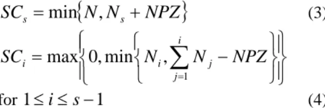
In this study, we also give the formulation of the number of rotational steps of the turret in each speed category i, (SCi). Assume that we partitioned the
component types into s groups according to their weight values, with group 1 being the lightest and group s being the heaviest. Then the following equations can be used to calculate SCi.
{
N
N
NPZ
}
SC
s=
min
,
s+
(3) ⎪⎭ ⎪ ⎬ ⎫ ⎪⎩ ⎪ ⎨ ⎧ ⎭ ⎬ ⎫ ⎩ ⎨ ⎧ − =∑
= NPZ N N SC i j j i i 1 , min , 0 max for 1≤i≤s−1 (4)where N denotes the total number of components to be populated, Ni represents the number of
components to be placed in group i and NPZ stands for the number of heads that are in no-pickup zone with NPZ ≥ 0. It is worth to note that the formulation has no recurrence relation and it is a general formula which works for any value of s for 1 ≤ s ≤ N. For the special case when s=1, i.e. there is only a unique weight category, we consider this unique group as the heaviest and apply Equation 3. Also, for i=1, Equation 4 can be reduced to
SC1=max{0,min{N1,N1-NPZ}}
which is equal to
4.2 Pairwise exchange procedure
In order to improve the algorithms, we designed a random search procedure. The procedure starts with a given solution and applies a number of pair-wise exchanges. Therefore we call it pair-wise exchange procedure (PEP). More specifically, it can be defined as follows.
Randomly determine two points (components) within group 1 (choosing among all groups will definitely worsen the total cost because; the basic idea of our algorithms is to place groups of components successively). If the new cost stays the same or decreases by exchanging these two points, perform the exchange. Continue this procedure until a predetermined number of exchange trials are made. We compared two different cost concepts. First one calculates the total cost of assembly and second one calculates the cost of placing group 1 components. The question here to answer is whether calculating cost of only group 1 components is adequate or not. This is important because after each exchange, calculating the total cost of assembly increases the computational cost, especially for large N values. We call applying the PEP according to total cost and applying PEP according to cost of group 1 as PEPTC and PEPCG1, respectively.
This procedure is applied after ATMA and iATMA. Thus we can say that starting solution to this procedure is either the route of ATMA or iATMA.
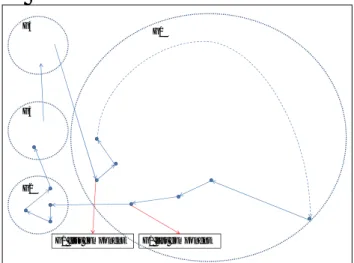
4.3 Further improvements
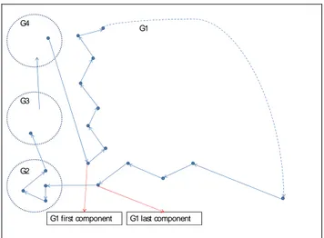
In order to obtain further improvements in terms of assembly time, new approaches can be proposed by taking advantage of inherent design of the analyzed PCBs. Figure 3 depicts a typical PCB produced in the industry. As observed in Figure 3, starting point for group 1 may stand away from its previous point in the sequence. Recall that, in ATMA firstly routes for each group are built and starting point for group 1 is selected (we preferred to select the one at southwest). Then, route 2 is connected to the last point of route 1 through shortest connection and route 2 is rearranged so that starting point of route 2 is the connection point. This adjustment is repeated for the route pairs (route 3, route 2) and (route 4, route 3), successively. After these adjustments, last point of route 4 may stand in a position that is far away from start point of route 1, as illustrated in Figure 3. When a continuous production is considered, the cost of this connection gains importance and its reduction should be sought. G2 G3 G4 G1 G1 last component G1 first component
Figure 3—Example depicting solution of ATMA
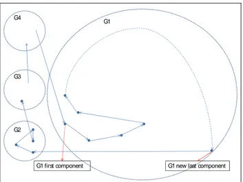
To cope with this deficiency, we propose making modifications to the solution obtained by ATMA. Altering the starting point of group 1 and selecting a closer point to the last point of group 4 is more meaningful than altering last point of group 4. This is because of the fact that number of components in group 1 is much more than number of components in group 4. Hence, we alter the start point of group 1 as the one closest to the last point of group 4. This must be done by preserving the last point of group 1, because other routes are already built according to last point of group 1. However, in this case some of the points (points between last point of group 4 and new starting point of group 1) are excluded from the tour and this situation raises the question of how to deal with these excluded components (see Figure 4). These components somehow must be inserted into the placement sequence.
G2 G3 G4
G1
G1 last component G1 new first component
Figure 4—The excluded vertices if starting point is altered.
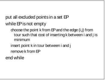
For inserting these components into the placement sequence, least cost insertion method can be used (Figure 5).
put all excluded points in a set EP while EP is not empty
choose the point k from EP and the edge (i,j) from tour such that cost of inserting k between i and j is minimum
insert point k in tour between i and j remove k from EP
end while
Figure 5—Least Cost Insertion Algorithm
Or discusses three different cost measures for inserting points into a tour [20]. These are difference, ratio and multiplication (difference times ratio) (Figure 6). We tried all of these measures, but we followed up the difference approach since it produced better results (see Table 3). We will call this method of insertion ATMAwithLCI (ATMA with least cost insertion) in the following discussions.
Table 3
—
Comparison of cost measures to be used in ATMAwithLCI Improvement acc. to ATMA ATMAwithLCI (cost1) 3,06% ATMAwithLCI (cost2) 1,13% ATMAwithLCI (cost3) 2,86%Cost 1 (difference) for inserting point k between points i and j:
distance(i,k)+distance(k,j)-distance(i,j)
Cost 2 (ratio) for inserting point k between points i and j:
(distance(i,k)+distance(k,j))/distance(i,j)
Cost 3 (difference x ratio) for inserting point k between points i and j:
Cost 1 x Cost 2
Figure 6—Cost measures
Note that the function distance(i,j) returns the cost of traveling from point i to point j in terms of time by Chebyshev measure, that is by considering turret time. Mathematically,
distance(i,j)=
max
{
t
ijx,
t
ijy,
t
t}
(6) where txij, tyij and tt are defined in section 2.2.Another method for inserting these excluded points can be defined as follows. The points starting from the point closest to new starting point of group 1, to the point closest to the last point of group 1 (points between a and b in Figure 7) are separated from the tour by preserving the order determined by Convex-Hull Or-Opt. Then insert this group of points between points i and j in the tour that gives the minimum total cost (total assembly time). In each insertion trial, both normal and the reverse order of the group is considered. This approach for inserting the excluded points is called ATMAwithGI (ATMA with group insertion).
G2 G3 G4
G1
G1 last component G1 new first component b
a
Figure 7—Connecting excluded vertices
A possible outcome of inserting excluded points into the tour is illustrated in Figure 8.
G2 G3 G4
G1
G1 last component G1 new first component
Figure 8—A possible outcome of inserting excluded points
One should keep in mind that the above discussions are valid for ATMA. A similar discussion can be made for iATMA by taking into consideration the inverse flow of placement sequence. As observed in Figure 9, the distance between last point of group 1 and first point of group 4 is very great and counts for an increase in assembly time when continuous production is considered. Hence, altering last point of group 1 should be investigated in this case.
G2 G3 G4 G1 G1 last component G1 first component
Figure 9—The solution that iATMA gives
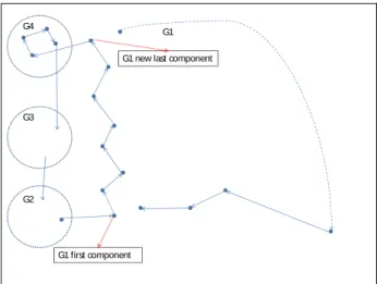
Finding the new last point for group 1 components is very easy. If we simply connect new last component of group 1 to first component of group 4, then we are faced with a situation as depicted in Figure 10.
G2 G3 G4
G1 G1 new last component
G1 first component
Figure 10—Connecting last point of group 1
In this figure we see that the excluded points from the tour are the ones that are on the right of the PCB. However, due to the inherent nature of analyzed PCBs, in most cases these excluded points are more than the points which are included in the tour. In this case, we will insert more number of points into a tour that has less number of points. Thus, it seems more rational to exchange the included points with excluded ones (Figure 11).
G2 G3 G4
G1 G1 new last component
G1 first component
Figure 11—Reversing the tour of group 1
Another important detail in this design is the rotation of the tour. Note that, it is required to reverse the rotation of the tour from start component of group 1 up to new last component of group 1.
After these adjustments, least cost insertion and group insertion methods are applied after iATMA. In the results section, they will called iATMAwithLCI and iATMAwithGI, respectively. We should note that, the mentioned three different cost measures for least cost insertion method are tried and we followed up difference (cost 1) approach because it produced better results (see Table 4).
Table 4
—
Comparison of cost measures to be used in iATMAwithLCI Improvement acc. to IATMA IATMAwithLCI (cost1) 0,77% IATMAwithLCI (cost2) -0,18% IATMAwithLCI (cost3) 0,66%Applying PEP after these methods should increase the improvement. Hence, we tried applying after ATMAwithLCI and ATMAwithGI techniques (also for iATMA variants). They are
called ATMAwithLCIwithPEP and ATMAwithGIwithPEP. Detailed results along with
their discussions of these techniques are discussed in section 5.
5
Conceptual Analysis and
Comparison of the Algorithms
5.1 Conceptual Analysis
The proposed iATMA generates a smaller LB than ATMA for the component placement problem. The following analysis proves this statement.
A data generator that produces random printed circuit boards is implemented. The position, type of the component and which category it belongs is randomly created. The methodology for this generator is the same as the one used by Duman [17]. The total number of components to be placed (N) is prespecified and it is given to the data generator. We studied with 4 different N values, 100, 200, 300 and 400. For N=100, the number of component types in groups 2, 3 and 4 are determined uniformly between 1 and 5, where each of them is placed one, two or three times (with equal probabilities) on the PCB. The rest of the components were in group 1 that is composed of 40 component types and the placement number of each one is probabilistically equal. For the larger problems (N=200, 300 or 400), the number of component types in each group is kept constant but their placement numbers are increased proportionally with N. The board that these components are placed is assumed to have dimensions of 250mm by 300mm and it is assured that no two components can be placed on the same coordinate.
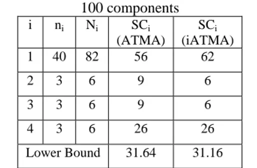
Table 5– LB values for both algorithms on a PCB with 100 components i ni Ni SCi (ATMA) SCi (iATMA) 1 40 82 56 62 2 3 6 9 6 3 3 6 9 6 4 3 6 26 26 Lower Bound 31.64 31.16
When the above data generation model is analyzed, one can easily see that in a typical PCB with 100 components (N=100), number of types of components and number of components to be placed for each group (Ni and ni values) can be expected as
follows: n1=40, n2=3, n3=3, n4=3, N1=82, N2=6,
N3=6 and N4=6 on the machine described in [17].
Applying the related formulas (Equations 3,4) for calculating number of rotational steps of the turret in a speed category i, (SCi) values for ATMA and
iATMA can be obtained easily (Table 5).
By applying Equation (2), the lower bound for this board is computed as 56*0.25 + 9*0.28 + 9*0.38 + 26*0.45 = 31.64 seconds for ATMA and 31.16 for iATMA similarly. This means that if all x-y movements of board carrier are completed within turret time, 1.5% improvement on the average can be obtained.
The same analysis can be applied when N=400 and one can obtain the following similar results in Table 6.
Table 6 – LB values for both algorithms on a PCB with 400 components i ni Ni SCi (ATMA) SCi (iATMA) 1 40 340 314 320 2 3 20 23 20 3 3 20 23 20 4 3 20 40 40 Lower Bound 111.68 111.20
It is interesting to note that the improvement that iATMA generates remains constant when N increases, and so relative improvement decreases to 0.4%.
5.2 Comparison on Synthetically Generated
PCBs
Up to this point, the expected benefits of algorithms are examined conceptually. Below, we will give simulation results.
Table 7
–
Assembly Time and LB values for both algorithms (Hom. boards)N ATMA iATMA Assembly Time Lower Bound Assembly Time Lower Bound 100 38.98 31.33 39.00 30.67 200 65.07 57.99 65.75 57.32 300 90.57 84.60 91.37 83.93 400 116.63 110.97 117.45 110.30
For the simulation study, the formerly introduced data generator is implemented and run to generate 100 different PCBs with varying N values from 100 to 400. The results are given in Table 7.
These values are exactly the same as the above conceptual analysis. The lower bound for iATMA is less than ATMA’s lower bound values for all N about the same amount of time. But the results also indicate a problem for iATMA. They indicate that even though iATMA is theoretically better than ATMA in terms of lower bound values, it is not superior than ATMA when placing the components for any N. So, as a result, it is proved that lower theoretical bounds can be obtained by placing groups of components in the reverse order (heaviest to lightest) but iATMA failed at reaching these lower bounds and even gave worse results. The possible cause of this situation is that in iATMA we face with the case max{ txij, tyij }> tt for consecutive
placement operations more than we face with it in ATMA. That is, the travel time from placement location to another is greater than turret time for more number of cases than predicted. If this travel time were smaller than tt, than we can achieve lower assembly times. The deeper analysis given below clarifies this discussion.
For each group, number of components placed in each speed category can be summarized in Tables 8 and 9 for ATMA and iATMA. The considered PCB board is the typical PCB board with 100 components described above.
Table 8 – Number of components placed in each SC for each group in ATMA
ATMA SC1 SC2 SC3 SC4
Group 1 Out of 82 56 9 9 8 Group 2 Out of 6 - - - 6 Group 3 Out of 6 - - - 6 Group 4 Out of 6 - - - 6
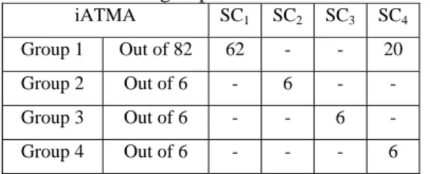
Table 9 – Number of components placed in each SC for each group in iATMA
iATMA SC1 SC2 SC3 SC4
Group 1 Out of 82 62 - - 20 Group 2 Out of 6 - 6 - - Group 3 Out of 6 - - 6 - Group 4 Out of 6 - - - 6
When generating the placements of components on a board the only consideration that we take into account is not to place two components on the same location. So the components in a group are randomly distributed over the board. When group 1 components are randomly distributed on the board and the TSP route for it is found, it is seen that the distance between two placements have reasonable length. That is, for most cases the travel time for this distance is not extremely greater than the turret time. But when other group components are randomly distributed on the board and the TSP route for it is found, it is seen that the distance between two placements do not have reasonable length. That is, for most cases the travel time of the board carrier for this distance is much greater than the turret time. So they cannot be placed in the turret time and an excess time is unavoidable. In the first table above (Table 8), we see that ATMA places these group 2, 3 and 4 components when the turret time is at maximum, i.e when the turret is at minimum speed that is during SC4. But iATMA places group 2
components during SC2 and group 3 components
during SC3, which is when turret is faster. So
ATMA compensates the possible excess time more effectively than iATMA, hence obtains a really big advantage. On the other hand, iATMA places more number of group 1 components in SC4 than ATMA.
But this will imply a small benefit for ATMA because, for most cases the travel time for this distance is not much greater than the turret time.
To summarize, to minimize the excess time occurring while placing the group 2, 3 and 4 components, placing them in minimum speed (SC4)
brings an advantage to ATMA and so it performs better.
A research on the design of placement locations of the heavier components reveal the fact that the components in the same group are preferred to be placed more closely. Their placement locations are mostly very close with one or two of them are far away from the group. That is, the distribution of heavy components throughout the board is heterogeneous. Thus we have two board models at hand, the board type in which all components are randomly distributed on the PCB and the model in
which heavier components are placed more closely. In this study, we will call the former one as
homogeneous model and the latter one as heterogeneous model. To obtain heterogeneous problem instances the data generator is re-implemented to give PCB instances in which heavier groups of components are placed more closely. On a board with this type of design, ATMA is expected to give worse results than iATMA because the disadvantage for iATMA disappears in this type of PCB instances. In Table 10, we give the results of the comparison of the PCB assembly time obtained by ATMA and iATMA. The PCB instances are created according to the modified data generator and each value is an average of 100 different PCB instances.
iATMA outperforms ATMA by 1.54% for N=100, by 0.47% for N=200, by 0.43% for N=300 and by 0.39% for N=400. This result could be expected because as N increases , the average x-y distances between component pairs decreases and it will be easier to arrange the placement sequence so that the board carrier movements can be completed within the free (turret) time by both iATMA and ATMA.
Table 10 – Assembly Time and LB values for both algorithms (Het. boards)
N ATMA iATMA Assembly Time Lower Bound Assembly Time Lower Bound 100 34.34 31.48 33.82 30.79 200 59.75 58.03 59.47 57.36 300 85.28 84.33 84.92 83.66 400 112.02 111.30 111.58 110.62
5.3 Pairwise exchange procedure
The results of applying variants of PEP (PEPTC, PEPCG1) after ATMA and iATMA along with their comparison discussion are as follows.
Table 11 – Improvement ratios of PEP variants after ATMA and iATMA on het. boards
In Table 11, we show the performance comparison of the algorithms on heterogeneous model PCBs with 100 components (N=100). Each total assembly time, average improvement and NOX value in the table is the average of 100 different PCB instances. Max column denotes the maximum improvement (percentage) value, Min column denotes the minimum improvement (percentage) value observed among 100 instances. The number of exchange trials set for PEP is 106, and NOX denotes the number of successful exchanges. NOCI denotes the number cases (instances) in which ATMA (or iATMA) is improved by using the relevant PEP variant, out of 100 instances. Percentage values are obtained by comparing each PEP variant by the relevant algorithm. For example, ATMAwithPEPTC improves ATMA by 0.24% on the average, 1.36% at best case and 0.00% at worst.
The
most general observation is that, applying PEPTC after both algorithms demonstrates better performance than PEPCG1, on the average. Also, it shows 0.00% performance in the worst case. This is an expected result of the study because design of this version is to make an exchange if total assembly cost improves. PEPCG1 is designed to make an exchange if cost of route 1 improves. But this exchange may accidentally increase total cost for the sake of decreasing cost of route 1 and hence may deteriorate the initial solution. This worst case may be observed in applying PEPCG1 after both algorithms but the following example (Figures 12 and 13) demonstrates the possible situation for ATMA in heterogeneous model.G2 G3 G4 G1 G1 last component G1 first component
Figure 12 – Example of a worst case that PECG1 may result on heterogeneous boards (Before PEPCG1)
Heterogeneous Boards Improvement Total
Ass.
Time Average Max Min
NOX NOCI ATMA 34.36 ATMAwithPEPTC 34.28 0.24% 1.36% 0.00% 5814 85 ATMAwithPEPCG1 34.33 0.09% 1.36% -2.05% 6035 65 iATMA 33.83 iATMAwithPEPTC 33.76 0.21% 1.30% 0.00% 8252 73 iATMAwithPEPCG1 33.79 0.12% 1.30% -1.36% 8273 65
G2 G3 G4
G1
G1 first component G1 new last component
Figure 13 – Example of a worst case that PECG1 may result on heterogeneous boards (After PEPCG1)
In Figure 12, an initial solution that ATMA produces is shown. The placement starts by first component of group 1 (G1 start component) and after traversing the group 1 components ‘G1 last component’ is reached. Then the tour is connected to group 2 components which is connected to group 3 and so on. PEPCG1 procedure makes an exchange, calculates the cost of placements of group 1 components and if it is improved then performs the exchange. Suppose that PEPCG1 makes exchanges and the last state of the tour for group 1 components is as in Figure 13. See that last component of group 1 (G1 new last component) becomes another component that is far away from group 2 components. Even though PEPCG1 makes the exchanges with the goal of decreasing cost of group 1 components, it accidentally performed worse. This example shows that how the connection from group 1 to group 2 components may increase and this increase may consume the possible benefit gained by PEPCG1 or it may even deteriorate the total cost.
Thus, using PEPCG1 rather than PEPTC may benefit in terms of computational cost by 15%, however PEPCG1 is more inconvenient than PEPTC. This can be seen by examining the maximum improvement and minimum improvement ratios. PEPCG1 may worsen the initial solution as much as 2.05% while it may improve the initial solution as much as 1.30%, which is the same as PEPTC. On the other hand, ATMAwithPEPTC outperformed ATMA in 85 cases and in the remaining 15 it gave the same result while ATMAwithPEPCG1 outperformed ATMA only in 65 models in the same 100 PCB instances, which is another indication of reliability of PEPTC.
When we consider applying PEPTC and PEPCG1 after iATMA, we reach the same
conclusion. iATMAwithPEPTC outperforms iATMA by 0.21% on the average, where the maximum gain is 1.30% and the minimum is 0.00%. As we described above, due to the design of PEPCG1, it may deteriorate the initial solution. This is again observed in iATMAwithPEPCG1.
From a general point of view, among all algorithms in Table 11, we observe that ATMA is improved by iATMA from 34.26 to 33.83 which is improved by PEPTC to 33.76 according to total assembly time, on the average. This brings about a 1.75% improvement, in total.
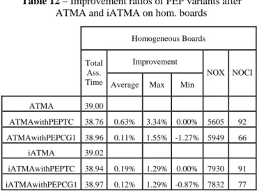
While introducing about heterogeneity of the PCBs, it is mentioned that mostly produced PCBs own this property. However, for integrity, the behavior of PEPTC and PEPCG1 on homogenous PCB model is presented in Table 12.
The discussions for the algorithms on heterogeneous PCB model can also be repeated for homogeneous boards such as the superiority of PEPTC over PEPCG1 when applied after both ATMA and iATMA, with respect to average, minimum and maximum values. They also show the same behavior when ‘number of cases improved’ is analyzed. However, there are some detail differences that are not observed in heterogeneous PCBs. The first point that attracts our attention is the great performance of ATMAwithPEPTC over others. It displays an improvement that others cannot. Even though the performance loss of iATMA is explained in previous sections, this is not the same case and deserves explanation.
Remember that while connecting the routes for group 2 components to group 1, ATMA connects them by shortest connection. But in homogeneous boards, especially when the number of group 2 components is very small (can be even only one component) and they can be far away from each other, the shortest connection between the routes may be as much away as the width or height of the board. The example given in Figures 14 and 15 depicts this situation.
G1 G1 last component G1 first component G2 G1 G1 G1 G1 G1 G1 G2 G2
Figure 14 – An example case where PEPTC improves ATMA (Before PEPTC is applied)
G1 G1 start component G2 G1 G1 G1 G1 G1 G1 G2 G2 G1 G1
G1 new last component
Figure 15– An example case where PEPTC improves ATMA (After PEPTC is applied)
In such a case, by performing exchanges, PEPTC after ATMA may change the placement sequence of group 1 components so that the last component of group 1 may be closer to first component of group 2 than before. PEPTC after iATMA can not benefit from the same scenario because in iATMA route of group 1 is connected to route of group 2. That is, after building routes for every group of components, route 3 is connected to (the last component of) route 4 by shortest connection, route 2 is connected to (the last component of) route 3 by shortest connection and route 1 is connected to (the last component of) route 2 by shortest connection. Hence despite the situation of having very few group 2 components, finding a close component to last component of group 2 among group 1 components is very easy.
Table 12 – Improvement ratios of PEP variants after ATMA and iATMA on hom. boards
Another issue that should be taken into consideration is the significancy of our contribution. Firstly, we formed the confidence interval for PEPTC after ATMA in homogeneous model and we are 99% confident that the mean performance gain (in percentage) is between 0.45% and 0.81% when compared with ATMA. This means that we are 99% confident that the mean performance gain (in seconds) is between 0,18 and 0,31. These results show that the performance improvement is statistically significant. Similarly, we formed the confidence interval for PEPTC after ATMA in heterogeneous model and we are 99% confident that the mean performance gain (in percentage) is between 0,17% and 0,30% when compared with ATMA.
The
probability values for t-tests are also worth to mention. t-test returns the probability associated with a Student's t-Test. We use t-test to determine whether two samples are likely to have come from the same underlying population that have the same mean. In homogeneous model, when the 100 values of ATMA and 100 values of PEPTC after ATMA are subject to t-test, we obtained 6,7E-15 probability. This means that the contribution of PEPTC to ATMA is very significant. We conducted the t-tests for PEPTC values with relevant ATMA and iATMA values in both models and, all tests gave almost zero probabilities as the one above. But t-tests for PEPCG1 values with relevant ATMA and iATMA values in both models gave about 0.01 probabilities, which can be referred as significant but not as strong as PEPTC tests.Thus, we show that applying PEPTC after ATMA or iATMA brings significant improvements to total assembly times of PCBs. We proved that in almost 90% of randomly generated PCBs, an improvement is possible, while for the rest the initial total assembly is preserved. PEPCG1 brings
Homogeneous Boards Improvement Total
Ass.
Time Average Max Min
NOX NOCI ATMA 39.00 ATMAwithPEPTC 38.76 0.63% 3.34% 0.00% 5605 92 ATMAwithPEPCG1 38.96 0.11% 1.55% -1.27% 5949 66 iATMA 39.02 iATMAwithPEPTC 38.94 0.19% 1.29% 0.00% 7930 91 iATMAwithPEPCG1 38.97 0.12% 1.29% -0.87% 7832 77
also some improvement but may also deteriorate the initial solution. In the following subsection, PEP will refer to PEPTC technique.
5.4 Further Improvements
The results of ATMAwithLCI, ATMAwithGI, ATMAwithLCIwithPEP, ATMAwithGIwithPEP,
iATMAwithLCI, iATMAwithGI, iATMAwithLCIwithPEP, iATMAwithGIwithPEP
along with their comparison discussion are as follows.
In Table 13, we show the performance comparison of the improvement techniques applied after ATMA on both homogeneous and heterogeneous model PCBs with 100 components (N=100). The values indicate the amount of percentage that ATMA is improved. We should remind that these results are an average of 100 different PCB instances. The first and most general observation in the table is that applying PEP after any technique definitely brings an improvement. From the table it can be seen that on heterogeneous boards, using ATMAwithLCI provides a significant improvement when compared with ATMAwithGI. When the same comparison is done by considering homogeneous boards, improvements of two insertion techniques stay almost at the same amount.
Table 13
—
Improvement ratios of insertion methods with respect to ATMAImprovement acc. to ATMA Hom. Boards Het. Boards
ATMAwithLCI 1,54% 3,06%
ATMAwithGI 1,66% 1,72%
ATMAwithLCIwithPEP 2,10% 3,34% ATMAwithGIwithPEP 2,69% 2,95%
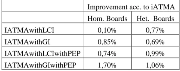
In Table 14, we show the performance improvements of the insertion techniques and PEP applied after iATMA. The values indicate the performance gain with respect to iATMA.
Table 14
—
Improvement ratios of insertion methods with respect to iATMAImprovement acc. to iATMA Hom. Boards Het. Boards
IATMAwithLCI 0,10% 0,77% IATMAwithGI 0,85% 0,69% IATMAwithLCIwithPEP 0,74% 0,99%
IATMAwithGIwithPEP 1,70% 1,06%
6 Conclusion
In this study, we proposed a new algorithm and improvement procedure for the solution of a problem faced in a particular PCB assembly machine. The machine type considered is a widely used one in the industry. Moreover, it has very similar properties with ‘chip shooter’ machines, especially when their rotational turret is considered. Thus, the improvement techniques discussed here could give useful insights for the assembly optimization of chip shooter machines.
The basic idea of the newly proposed heuristic is to mount the components in reverse order of a previously proposed approach. The previous approach categorizes components into groups according to their weights. Then it places the components in the order from lightest to heaviest. Our approach places the components in reverse order, from heaviest to lightest. That is why it is called inverse ATMA (iATMA). This method brings an improvement about 1.54% for a board having 100 components. Furthermore, some random search heuristics are investigated in order to improve iATMA. Pair-wise exchange procedure is applied after ATMA and iATMA. Moreover, by taking advantage of inherent design of the analyzed PCBs, promising approaches for minimizing total assembly time are also suggested. These techniques are based on connecting two routes from shortest connection and inserting the temporarily excluded points. By applying all the developed techniques to the problem instances, performance improvement figure reaches up to 4.50% when compared with previous studies.
The future work would be to investigate the possible improvement that may be obtained by redesigning the route for group 1 components using prize collecting TSP or Heterogeneous Vehicle Routing Problem approaches. Another method that we plan to investigate is the simulated annealing meta-heuristic which is proven to give promising results in combinatorial optimization problems. Also, the methods developed in this study will be generalized to chip shooter machines.
References:
[1] Duman, E., Optimization Issues in Automated Assembly of Printed Circuit Boards, PhD Thesis, Bogazici University, 1998.
[2]