Coordination of production and advertising decisions in a single period with a budget constraint

(1)

COORDINATION OF PRODUCTION AND ADVERTISING DECISIONS IN A SINGLE PERIOD WITH A BUDGET CONSTRAINT

A THESIS

SUBMITTED TO THE DEPARTMENT OF INDUSTRIAL ENGINEERING

AND THE INSTITUTE OF ENGINEERING AND SCIENCES OF BILKENT UNIVERSITY

IN PARTIAL FULFILLMENT OF THE REQUIREMENTS FOR THE DEGREE OF

MASTER OF SCIENCE

by Ateş Gözek

(2)

COORDINATION OF PRODUCTION AND ADVERTISING DECISIONS IN A SINGLE PERIOD WITH A BUDGET CONSTRAINT

Ateş Gözek

M.S. in Industrial Engineering Supervisor: Prof. Dr. Ülkü Gürler

June 2006

In this study, we consider the production and advertising decisions in a newsboy setting with a budget constraint. Regression models that elaborate the effects of advertising on sales are investigated and various sales response models are presented. An application in soluble coffee market is also provided. Linear and power response functions are incorporated to jointly consider the production and advertising expenditures in a single period newsboy setting. Our numerical analyses indicate that production and advertising expenditure percentages are more sensitive to budget than the lost sales cost and the uncertainty (variance) of the demand.

(3)

ÜRETİM VE REKLÂM KARARLARININ TEK PERİYOTTA, BÜTÇE KISITI ALTINDA KOORDİNASYONU

Ateş Gözek

Endüstri Mühendisliği Yüksek Lisans Tez Yöneticisi: Prof. Dr. Ülkü Gürler

Haziran 2006

Bu çalışmada, üretim ve reklâm kararları, gazeteci çocuk kurulumu içinde, kısıtlı bütçe altında incelenmiştir. Reklâmın satış üzerindeki etkisini açıklayan regresyon modelleri araştırılmış ve birçok satış tepki modelleri sunulmuştur. Çözülebilir kahve piyasasından bir uygulama verilmiştir. Üretim ve reklâm harcamalarının bir arada incelenmesi için lineer ve güç tepki fonksiyonları tek dönem gazeteci çocuk problemine dâhil edilmiştir. Sayısal analizlerimiz, reklâm ve üretim harcamalarının, bütçe kısıtına, talep belirsizliği ve kaybedilen satış maliyetinden daha duyarlı olduğunu göstermiştir.

Anahtar Kelimeler: Reklâm, Satış Tepki Fonksiyonları, Gazeteci Çocuk Problemi.

(4)

I would like to express my sincere gratitude to Prof. Dr. Ulkü Gürler for all the encouragement and trust during my graduate study.

I am indebted to members of my dissertation committee: Asst. Prof. Emre Berk, Asst. Prof. Osman Alp for showing keen interest in the subject matter and accepting to read and review this thesis. Their remarks and recommendations have been very helpful.

I would like to thank Önder Bulut, Mehmet Fazıl Paç, Sibel Alumur, and Muzaffer Mısırcı for their help, friendship and support.

(5)

1 INTRODUCTION...1

1.1 Coordination of Marketing and Manufacturing……….1

1.2 Basic Concepts Regarding Advertising……….5

2 LITERATURE REVIEW ...10

2.1 Marketing Strategies ...10

2.2 Coordination of marketing and manufacturing activities ...21

3 ADVERTISING -SALES RESPONSE FUNCTIONS ...25

3.1 Empirical Results of Sales Response Functions ...25

3.2 Commonly used Sales Response Function ...26

3.3 An Application on Coffee Sales ...30

4 SIMULTANEOUS DECISION MODEL FOR PRODUCTION AND ADVERTISING ...35

4.1 The Single Period Newsboy Problem ...35

4.2 Integration of the Demand Response Function into the Newsboy Problem………...37

4.2.1 Linear Demand Response Function………37

(6)

5 A NUMERICAL EXAMPLE……….42

5.1 The Data Set………...……….42

5.2 Estimation of the Demand Response Function…………...……….... 43

5.3 The Newsboy Formulation………...………49

5.4 Cost and other parameters……..……… 49

5.5 Results………...………..…... 51

6 CONCLUSIONS AND FUTURE RESEARCH DIRECTIONS ...58

BIBLIOGRAPHY ...62

APPENDIX A ...67

APPENDIX B...71

(7)

3-3: Coffee sales in natural Logarithm from January 2002 to December 2003 31

3-3: Normal Probability Plot of Error Terms... 32

3-3: Standardized predicted values versus standardized residuals scatter plot . 33 5-1: Monthly sales quantity and related advertising expenditure... 43

5-2: Curve Fitt Plots for Regression Models... 44

5-2: Curve Fit Plot of the Power Response Function ... 45

5-2: Normal Probability Plot of Error Terms... 46

5-2: Standardized predicted values versus standardized residuals scatter plot . 47 5-2: Sales for different advertising expenditure values ... 48

5-2: Sales versus advertising expenditure when

β

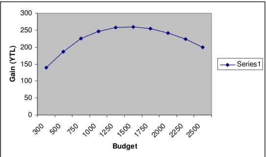
₁ =0.2... 48

5-5: Gain values for increasing budget, when ,p λ=5 and σ =0.39 ... 52

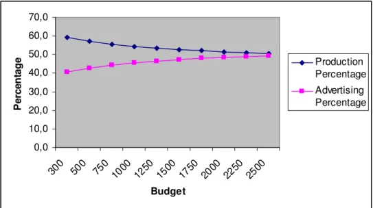
5-5: Percentage of production and advertising levels for different budgets when λ=4,σ =0.38,p=6. ... 53

5-5: Percentage of production and advertising levels for different budgets when λ=5,σ =0.40,p=6... 54

(8)

5-5: Percentage of advertising expenditure for increasing levels of standard deviation for budgets 5000 and 2000 YTL... 55 5-5: Service levels for increasing percentage of advertising expenditure for

0.38

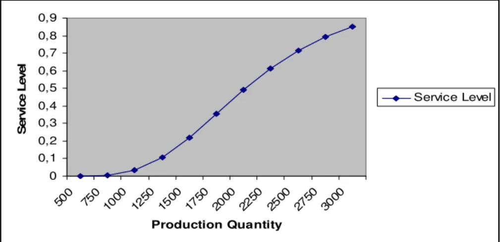
σ = ... 56 5-5: Service levels for increasing production quantity when A =500 and

0.38

σ = ... 56 Appendix B: Service levels for increasing production quantity when budget is 5000 YTL and σ =0.38... 81 Appendix B: Service levels for increasing production quantity when budget is 5000 YTL and σ =0.46... 81 Appendix B: Service levels for increasing production quantity when budget is 2000 YTL and σ =0.38... 82 Appendix B: Service levels for increasing production quantity when budget is 2000 YTL and σ =0.46... 82 Appendix B: Gain, production quantity, and advertising expenditure plot for

(9)

3-2: Commonly used Regression Models ... 28

A-2: Monthly Coffee Sales and Related Advertising Expenditures for the years 2002-2003 ... 67

A-3: Regression Statistics for the Coffee Sales ... 68

A-4: Coefficients of the Regression Model ... 68

A-5: Monthly Sales Quantity and Related Advertising Expenditures ... 69

A-6: Model Summaries of Curve Estimation ... 70

A-7: Regression Statistics ... 70

5-4: Experimental Set ... 50

INTRODUCTION

1.1 Coordination of Marketing and Manufacturing

Companies become aware of the fact that reaching out the customers, understanding their needs, and providing them the best service are the key elements to acquire a strong position in the market. Moreover, increasing competition between the organizations force them to reduce the cost of their production activities. Hence, the marketing and the manufacturing departments stand as the most important units of an organization. Not only do the advertising strategies and profitable manufacturing individually help companies to reach their goals, but coordination between these activities assist organizations to do their best in terms of the performance criteria. Considering the marketing activities, advertising is the most powerful tool to attract the customers; therefore, its impact on sales is considered to be an important and a valuable information to assist the coordination between the two departments.

Advertising has its roots in ancient times, as a cost effective way to disseminate messages. Archaeologists have found evidence of advertising dating back to the 3000s BC, among the Babylonians. One of the first known methods of advertising was the outdoor display, usually an eye-catching sign painted on the wall of a building. The modern advertising today, had its

(12)

beginning in the mid 1800’s. After 1920 s advertising became an effective tool in modern marketing. Due to increasing competition in market sectors, advertising digress from traditional business patterns, and applied in a more professional manner.

Advertising can be considered in three different perspectives. From the consumer’s point of view, it is a collection of messages informing them about the goods or services. From a societal perspective, advertising is a valuable service to community; it helps consumers to understand the ideas, differences between the product brands, and distinguishing aspects of companies and institutions, by informing them through paid media. The most common and important perspective is that of business. Advertising is an effective, persuasive marketing communication program directed towards target buyers or distributors to successfully market any product or service. Increasing sales is the main objective of advertising.

Apart from marketing activities, the manufacturing department is the most important unit of a company. It is responsible for the production, the quality of the products, capacity utilization, delivery times, and introduction of the new products into market. However, the company has to know and minimize its costs to stay in the market. Interaction between manufacturing and marketing departments plays a vital role for the company to effectively manage the inventory system. Although these departments both have different objectives, point of views and work styles, one of them would not operate efficiently without the other.

Manufacturing department requests more accurate sales forecasts, and reasonable promises to customers from marketing department whereas,

(13)

marketing department would want higher capacity utilization, on time delivery, quality assurance and minimum cost from manufacturing department. If the marketing department comes up with a poor sales forecast, it would cause the manufacturing department to produce more and end up with higher inventory than planned which eventually incur higher costs to the company. On the other hand, if the manufacturing department could not operate with an accurate sales forecast, the company would lose sales by not supplying sufficient amount of products. Moreover, if the manufacturing department does not meet the product quality or on time delivery promises given by the sales personnel to customers, the company would lose the goodwill which will eventually lead to losing customers and hence profit.

An increased and effective coordination between the manufacturing and marketing activities would help improving the overall efficiency of the firm. Sharing information might enable marketing to adjust their forecasts, and helps manufacturing department to have more control on the capacity quality and delivery deadlines. For instance, due to production capacity restriction, Honda Company did not broadcast its last commercial in Turkey and many other countries, where an orchestra imitates the sound of a 2006 Honda Civic while its travels on a highway. Effective evaluation of the commercial’s effect on sales, and share of information between marketing and manufacturing departments prevent the Honda Company from loosing brand loyalty. For a negative example, when Doritos Alaturka broadcast the series of commercials featuring Cem Yılmaz, they had to stop broadcasting for a period since; Doritos could not produce enough to supply increasing demand. Sales had a potential to increase; however, Doritos had to stabilize the demand to not to lose brand image and customers. Consequently, harmonizing manufacturing,

(14)

and marketing departments’ activities would help the company to minimize their costs, increase their profits, and acquire brand loyalty.

In this study, a joint decision model for production and advertising activities is presented. We considered a firm with a limited budget for advertising and production. The effect of advertising expenditure on sales is investigated through a sales (demand) response regression model. After assessing the effects of advertising on sales, we focused on the production problem.

A classical newsboy formulation with the incorporation of the response (demand) function is used. Two different response models, namely a linear and a power function are considered. A profit maximization problem to optimize production quantities and advertising expenditures with different budget constraint is constructed. The resulting model is investigated with numerical methods. A data set that consists of sales quantity and related advertising expenditure for a period of eighteen months is examined to acquire the response model. For this particular example power response function is found to be the best explanatory model, hence is integrated in the newsboy problem. Then the expected profit is maximized with nine different budget constraints. For every budget constraint different product price, lost sales cost and variance of the response model is examined to exploit the effects on expected profit. It is found that, an increase in the lost sales cost forces the firm to increase the production quantity to avoid unsatisfied demand; in addition, the firm decreases its advertising expenditures to a point where the lost sales will be minimized. When the price is higher than the lost sales cost, the increase in the profit diminishes depending on the variance. As we increase the variance, the difference between the profits for increasing budget limits will descend. We obtained the budget points where our gain starts to decrease with the increase in the budget. In addition, we present a sales response model,

(15)

which we construct by analyzing a data set from one of the biggest food production companies in Turkey. The data set consists of the monthly sales and related different advertising expenditures (i.e. television, outdoor, radio, internet etc.) for a soluble coffee for the years 2002-2003. Regression analyses give a linear response model including lagged variables. The integration of this model into the production problem complicates our analyses, the problem could not be solved in a single period model; therefore, we suggest the problem as a future research.

We next want to discuss some basic concepts regarding advertising and the effect of advertising on sales.

1.2 Basic Concepts Regarding Advertising Types of Advertising

Depending on the stage of the product in the market, three different types of advertising can be used to affect the consumers and to increase sales. Informative advertising has been used frequently in the very early stages of a product category, to create a general level of awareness in the target population. Telling the market about the new product, informing consumers about different prices, explaining the new uses of the product, describing available services help marketers to build a company image and let them be known in the sector.

After public awareness is achieved, the competitive stage begins. Persuasive advertising has been used heavily to bring the consumer to a point of purchase which can take minutes, hours, days or months. Since the ultimate goal is increasing sales, a selective demand is needed to be built. In this stage,

(16)

advertiser encourages the consumers to switch to their brand, and tries changing the consumer’s perception of product or service attributes. Hence, comparison advertising tactic is mostly used to establish the superiority of the brand.

Reminder advertising can be thought as a device to keep the brand name fresh in the minds of the consumers during off seasons, by telling them that the product may be needed in the near future, or informing them about the possible places to buy the product. Maintaining brand loyalty rather than market share is the primal aim in reminder advertising for a company. Burger King, Coca Cola, Nestle, Volkswagen are some of the examples that use reminder advertising frequently. After setting the objectives, deciding on the budget, and selecting the message and media type to communicate, and the final and most important stage, evaluating the effectiveness of the advertising program, is needed to be carried out.

Assessing the Sales Effects of Advertising

Assessing the effectiveness of advertising consists of two basic concepts. Measuring the communication effect, and the sales effect of advertising. Copy testing is used to acquire feedback from consumers about whether an advertisement is communicating effectively. Both professional advertisement agencies and marketing managers agree that copy testing is a valuable tool to diagnose checks the components of the advertisement campaign. For example, a pretest program, where a sample of target population is exposed to a television or a magazine ad, and then asked for their opinion about the ad’s believability, perception of the message, and their feelings about the ad, might give important information to marketers whether to carry out the campaign, or

(17)

if needed, do the necessary corrections which might be the length, message or timing of the ad, while saving the whole advertisement budget. If an advertising campaign is completed, then advertisers might also be interested in post testing the effectiveness of the campaign using the same methods such as attitude and opinion studies, memory tests and etc. Since increasing sales is the main objective, measuring the sales effect of advertisement campaign become a must for the marketers.

Assessing the sales effect is generally harder than measuring the communication effect; companies wish to know if they allocate enough, overspending, or underspending on advertising. There exist many variable factors influencing sales such as price, features, and availability of both the company’s and its competitors’ products; moreover, seasons, rapidly changing consumer tastes and values in addition with the cumulative and lagged effects of the advertising campaigns make it hard to correlate advertising performance with sales.

Direct measurement is one of the three ways that companies use to evaluate sales effect of advertising. This method is usually implemented by television ads or programs that demonstrate the products and contact information is provided. Sales made through this contact information are attributed to the television commercial and hence it is possible to detect the effect of the advertising campaign.

Experimental design is another method that enables marketers to measure the sales effect of advertising indirectly. This method is a controlled experiment which the marketer manipulates an advertising decision variable in a performance area, while controls the other variables in another area.

(18)

Unfortunately, it is not possible to test more than one factor at the same time in the test area. This method has major drawbacks. It is time and money consuming to design and apply the experiment. Realization of the lagged effects might require many months; furthermore, competitors would have a great deal of knowledge about the campaign and its results. In store data is generally used for controlled experimentation.

Finally, sales (demand) response models have been used to measure the effect of advertising for over forty years. In marketing literature, regression models have been heavily used to understand the impact of advertising on sales. The marketer collects information about the factors that he considers to be effective on sales (demand) such as advertising expenditure, the price of the product, the market share of the brand, promotional activities (price discounts, coupons, prizes etc.), placement of the product in the shopping center, brand loyalty, competitors’ prices, competitors’ advertising activities and possibly the lagged effect of these variables and many more. Then a regression model is constructed that uses these variables. However, one should be very careful when examining the regression equations; since all the variables in the model can be correlated with sales as well as they can be correlated with each other. The more variables used in the model, the higher the coefficient of determination (R2) would be achieved. However, if some of the variables are highly correlated with each other, then the model would not reflect the true effect of these factors on sales. Some elimination methods such as backward and forward elimination and some special regression models where the correlations between factors are minimized are used. Consequently, the marketer can obtain a highly reflective and accurate model after some set of analysis; hence evaluate the effect of various advertising activities. In our

(19)

study we used two regression models in order to express the relation between the sales and the advertising expenditure.

The rest of the thesis is organized as fallows. In Chapter 2, a literature review about advertising-promotion and sales (demand) relationships, and advertising- production and profit maximization relationships is provided. In Chapter 3, important assumptions for sales-advertising functions and various types of sales (demand) response functions including our analyses for the food production company are presented. In Chapter 4, the newsboy problem with the integration of two different types of demand response functions is stated. Then, the profit maximization problem with a budget constraint consisting of advertising plus production costs is demonstrated. In Chapter 5, a numerical example is provided. First, effects of advertising expenditure on demand are presented by a linear regression equation, and then expected profit is searched by our newsboy problem where developed demand response function is placed as the demand function. Eventually, a profit optimization problem and the results are stated. Finally, in Chapter 6, conclusions general results and extensions are provided.

(20)

C h a p t e r 2

LITERATURE REVIEW

In this chapter we review the basic literature related to our research. We first consider the studies related to marketing strategies and response models in section 2.1 and in 2.2 we review the studies that consider advertising and manufacturing activities jointly.

2.1 Marketing Strategies

Studies concerning advertising and promotion have been dealt extensively after 1970’s. Most of the research concentrated on optimal advertising strategies, budget allocations for advertising and promotion, effects of promotions in consumer purchases, retailer and consumer responses to discounted prices and trade promotions, and advertising and promotion strategies for long run profitability.

One of the first studies related to advertising is by Zufryden [19]. He demonstrates two optimization models to aid marketing executives in advertising budget allocation in decision-making. His two advertising response models examine the time pattern of market share for a particular product brand as a function of advertising expenditures and the dynamics of the market environment. In the formulation of the optimization model, essential

(21)

components of the model are steady state market share to determine the long run implications of advertising strategies, market share pattern as a function of time, and cumulative sales. Decreasing competitive advertising, increasing competitive advertising, and competitive advertising set as proportion of sales are the three scenarios in determining the optimal multi period advertising expenditures.

Another budget allocation model, using response functions that can express cause and effect relationships (i.e. sales and advertising budget), and an optimization model as Zufryden is presented by Hotthausen, and Assmus [8]. They concentrate on the allocation of an advertising budget to geographic market segments when the sales response to advertising in each segment is characterized by a probability distribution. They classify the allocation by the resulting expected profit and its variance. Optimizing the expected profit for different values of risk (variance), enable them to acquire mean-variance pairs. Different from Zufryden, they use sales for the territories as the dependent variable to their response functions, and expected profit in their optimization model instead of market shares. Two alternative sales response functions are developed: one assumes that the variance of sales in each segment is an increasing function of the advertisement expenditure, while the other assumes that the increases in variance occur as the advertisement level deviates from some usual or benchmark amount. After an efficient frontier for the expected profit has been established by different mean-variance pairs, management can choose one allocation among efficient allocations for different risk preferences.

Different from previous budget allocation studies, Kinberg et al. [11] concentrate on the problem of allocating fixed resources between spot demand

(22)

and package (subscription) demand. Two models are presented. In Model 1, a probabilistic spot demand, for a single resource, stationary over time, is assumed together with externally determined spot and package pricing. In Model 2, package price is considered to be a decision variable. The allocation policy derived from these models enable managements to set targets that should be periodically reviewed subject to changing demand and sales information, for package-subscription volume for their marketing personnel under changing market conditions.

Mesak and Means [14] work on optimizing advertising budgets and their allocations over time for both concave and S shaped attraction functions in a symmetric oligopoly by using the modified multinomial logit model (MNL) of market share. As Hotthausen and Assmuss, they try to maximize the profit, and similar to Zufryden they concentrate on the market shares. However, they reach to preferable advertising policies for different attraction functions. Due to exponential nature of the present MNL model, profit maximization is gained by increasing advertising as much as possible. Their modified function successfully represents the situations of diminishing returns to scale. In optimizing the advertising models in a symmetric oligopoly, they assume all N firms have same production costs, charge the same fixed price, face symmetric demand functions, to be able to acquire real promotion on the same terms, and to have similar market shares. They conclude that, if a firm has a concave attraction function or a high advertising budget under S shaped attraction function, Uniform Advertising Policy, where the marketer advertise on a constant rate for the whole period, would be the best choice. Moreover, Advertising Pulsing Policy would be beneficial for a firm with a small advertising budget in the presence of S-shaped attraction function. Finally, regardless of the shape of the advertising attraction function of the firm, the

(23)

advertising budget of the firm should increase with an increase in its gross profit margin.

Neslin, et al. [15] examine the effects of four types of promotion, coupons, manufacturer and retailer advertisements, and price cuts in terms of the acceleration of the product purchases characterized by two forms: purchasing a larger quantity, and shortening of interpurchase time. Moreover, they compare different market segments and loyalty groups. They present the impact of promotion with two regression models considering the quantity purchased and interpurchase time respectively. A scanner data from three major area supermarket chains applying everyday low price policy is used. They showed that purchase acceleration happens due to increased purchase quantity rather than shortened interpurchase times. In addition, advertised price cuts claimed to be the most effective tool of accelerating purchases.

Sasieni [17] considers advertising policies for a class of response functions. He prefers awareness instead of sales with rate of advertising in his model since the awareness and sales has the same mathematical structure. He shows that if a pulsing policy is used, awareness would reach to a steady state, and the average response function over the cycle is a decreasing function of the length of the cycle. If response shows increasing returns to scale he uses a device chattering to replace the true response by a straight line. Hence, optimal policy can be computed, when part of the response is linear.

Assuncao and Meyer [1] study the rational effect of price variations (promotion) on sales and consumption in a dynamic market environment. Their study presents a stochastic point of view into the subject. They first present a theory of sales response to price promotions. Price is assumed to be a

(24)

random draw from a stationary distribution of prices conditional on the last observed price that captures the buyer’s expectation of future prices. According to buyer’s inventory and good’s observed price, the optimal purchase quantity and consumption policy is given by the optimization model presented.

As Assuncao and Meyer, Kopalle et al. [12] also study the dynamic effect of discounting on sales. They develop a descriptive dynamic brand sales model to determine the normative price promotion strategies and to analyze the trade off of promotion and its negative future effects i.e. Decrease in reference prices, increase in stockpiling, more price sensitive customers, and lower baseline sales. They use 124 weeks of A.C. Neilsen store-level data of a liquid detergent due to its stockpilability, and frequent discounts. They refer to Foekens et al (1999) for their dynamic SCAN*PRO based model. They construct an empirical analysis including six brands. Their results suggest that brands with higher shares tend to over-promote; however, brands with lower shares do not promote frequently enough. With the results of the dynamic model, they aim to find the optimal retailer and manufacturer prices over time.

A problem where a retailer or a manufacturer wants to estimate product price and promotion elasticities, is studied by Blattberg, and George [3]. They propose shrinkage estimation procedures reducing the variability, at the same time providing flexibility allowing for separate elasticity estimates. Similar to Kopalle et al. a sales (brand-chain) regression model including the promotion effect variables is constructed. When compared against rank regressions, Ordinary Least Squares estimation gives highly satisfactory results concerning the linearity of the model, residual assumptions, and robustness of the model; however, high intermodel variability caused coefficient estimates to have

(25)

wrong signs. Therefore, they propose an alternative model that treats each of the chain brand model as separate and unrelated. Model shrinks the estimators, so that undesired variation could be prevented. They conclude their work with a comparison of the Ordinary Least Square estimation, and Shrinkage estimation procedures.

Neslin, Powell, and Stone [16] focus on the retailer’s and consumer’s response influence on a manufacturer’s optimal advertising and promotion plans. They concentrate on two main questions: The level of the expenditures for advertising and trade promotions, and how these expenditures should be scheduled. They formulate and analyze a dynamic model describing the activities of three parties: A single manufacturer, a set of retailers, and a set of consumers. Their main result express that, the decreasing and increasing consumer receptivity to promotion and advertising induce a negative relationship between promotion and advertising expenditures of the manufacturer.

Blattberg, Briesch, and Fox [4] present findings across the sales promotion literature. They identify and explain empirical generalizations related to sales promotion. They also focus on the conflicting findings in the research. Moreover, they briefly identify the sales promotion topics that have not yet been studied.

Cooper et al. [6] present an implementation of a promotion event forecasting system PromoCast™ for consumer packaged goods industry to provide short-term tactical forecasts useful for promotions from a retailer’s point of view. They involved 95-185 grocery chain stores in their research. They construct a 67-variable regression-style model. Promotional mix, items promotional

(26)

history (base line sales, promotion style), and each stores historic relation between a particular style of promotion and the resulting sales are the three perspectives led them to develop the model. Historical base line average sales were the strategic assets for their forecast.

Bell et al. [2] focus on decomposition of elasticities across brand choice, purchase incidence, and stockpiling. Moreover, they try to explain variance in promotional response that they decompose into primary and secondary demand components. Their study consists of 173 brands across 13 different product categories. They define the promotional response as the consumer’s reaction to a price promotion. Category-specific factors, brand-specific factors, and the consumer characteristics are the three aspects that the variance in promotional response is driven by. They conclude that the largest percentage of the elasticity decomposition falls on the secondary demand, or brand switching, in addition, category-specific factors are more powerful than brand-switching factors in explaining the variability in elasticities.

For the management of advertising and promotion for long run profitability Jedidi et al. [9] focus on three questions. One, whether to advertise or promote, two, whether it is better to use frequent, shallow promotions or infrequent, deep promotions, and finally, how changes in regular prices affect sales relative to increase in rice promotions. They introduce a heteroscedastic, varying-parameter joint probit choice, and regression quantity model. At the end, they conduct simulations to asses the relative profit impact of long term changes in pricing, advertising, and promotion policies. They concentrate on consumer choice of brand, and consumer’s quantity decision given that choice of brand in their model. They include long term marketing variables (Advertising), and consumer specific factors (brand loyalty). In order to

(27)

capture how consumers respond to price changes, and how they adapt their responses to changes in advertising and price promotions over time, they introduce a utility function. They reparameterize price and promotion as functions of long term advertising, long term promotion, and brand loyalty in a regression model. In their quantity model, while price and promotion have the same operalization as in choice model, they include inventory parameter to capture the effect of stockpiling in previous purchase occasions on future purchase quantity decisions. They conclude that, in the long term advertising has a positive effect on “brand equity” while promotions have negative. Moreover, promotions make consumers more price sensitive, and less discount sensitive in their brand choice in the long run. In addition, promotions make it difficult to increase regular prices.

Similar to Jedidi et al.[9], Zhou et al. [18] investigate the impact of short term advertising on long term sales of consumer durables and nondurables. Contrary to the common belief among marketing managers that regardless of the sales, long term advertising is better than short term, they claim that short term advertising campaigns can have long lasting impact on sales. Hence, corporations can use their marketing budgets more effectively through cutting advertising wastage. They explore the consumers’ profiles and behavior. For example, consumers are highly involved and selective when buying durables to reduce risk. Therefore, advertising creates a long term “memory” effects on buyers. Secondly, advertising gives consumers an incentive to make both an initial purchase and repurchase. In the case of nondurable products, consumers are passive audience to advertising and pay little attention to ads before the purchase. Therefore, they expect to find out that a significant advertising persistence effect is less likely to be found with the sales of consumer nondurables than with durables.

(28)

They collect television advertising and sales data for 14 brands of durables and nondurables in Shangai, from January 1996 to September 1999. They design their model to isolate the effects of television advertising from other effects such as marketing environmental variables like price index and wage index. They consider four scenarios to examine the relationship between sales and advertising expenditure. Business as usual (temporary advertising activity that creates temporary sales results), hysteresis (temporary advertising activity that results in sustained sales changes), evolving business practice (sustained advertising activity that are accompanied by persistent sales, and finally escalation (sustained advertising activity that are accompanied by increased long term sales due to unexpected factors). Their sales model is consist of lagged sales at a particular time, marketing activity, and environmental variables. They apply unit root test for non stationary variables, and cointegration test. The series that qualify for both of the tests are used in the model. Consequently, they conclude that, advertising have long term effects on sales of consumer durables, but did not have long term effects on sales of consumer non durables. Moreover, the dynamic evolvement of sales is related to consumers’ level of involvement with the product in making purchase decisions. Finally, they suggest that periodic advertisement instead of continuous advertisement for consumer durables would be more cost effective, and non durables need more continuous or sustained advertisement.

Bhargava, and Donthu [5] study the effects of outdoor advertising on sales. Outdoor media is available to reach consumers in a specific geographic area, and to create awareness fast. Geographically segmented markets, the traffic flow, the location of the billboard and geographic distribution of the target customers are considered as the spatial effects. They also study the temporal effectiveness of outdoor advertising where their aim was to generate short

(29)

term response with minimum exposures with lower advertising cost; nevertheless, as effective as many exposures. They conduct two field experiments in one of which they used billboards with a promotional message to increase the attendance (sales) to a Muttart Conservatory displaying flora and fauna from around the world. Visual observations are tested with statistical methods. They compare the density plots of previous and current year. For every zip code area, the number of customers attending to Muttart before the campaign and after the campaign, and the number of billboards are computed. It is clear that the number of billboards in a zip code area are highly correlated with the increase in the number of people attending the institution. Analysis of Variance is performed to measure the spatial and promotional effectiveness of outdoor advertising. Their results show that billboards are the most effective factor with the locational and promotional factors. Secondly, they conduct an experiment for a sports complex. This time they use multimedia advertising, newspapers and billboards. They divide the city in four zones. A control zone (no advertising), newspaper only, billboard only, and multimedia (both newspaper and billboards). Weekly usage data of the complex for the year of campaign and the previous year’s are collected. Time series analyses show that the campaign is successful. However, they also want to examine the effects of media separately, hence analysis of variance is conducted. They conclude that outdoor advertising produces shot term sales, they are more effective when used with multimedia, and they increase sales more when they have a promotional message.

Jagpal et al. [10] propose a different model than distributed lag and autoregressive sales models. They claim that the lagged and autoregressive sales specifications used to estimate the sales response functions, does not fully take into account the effects of cumulative advertising, moreover, these

(30)

models give little attention to interactions among elements of the marketing mix. They aim to propose less restrictive models to detect marketing mix interactions, and cumulative effects of advertising while checking the validity of distributed lag and autoregressive sales models. In their model, they exclude the lagged sales effect instead they include multiplication of advertising expenditure in current and past periods in a log linear distributed lag form. Consequently, they acquire variable returns to advertising, they are able to examine both past and present marginal effectiveness of advertising, and instead of constant elasticities, they allow for flexible current sales and cross elasticities. They use monthly sales advertising data from a vegetable medicine to test their model. By ordinary least square estimation, they find the significant lags that they would use in the regression equation.

Finally, according to their analysis, they conclude that Multiplicative Nonhomogeneous Sales Functions fit the data better than distributed lag models, plus it is capable of detecting a threshold level below where advertising is ineffective hence, by Multiplicative Nonhomogeneous models, they are able to reallocate the advertising budget more accurately, since it points out the departures from optimal advertising by analyzing the marginal elasticity results.

Kumar et al. [13] focus on trade promotions in their research. In their system, there exists a single manufacturer serving two consumer segments through a single retailer. They analyze the strategic issues that underlie the retailer’s decision to pass through the trade deals. They conclude that the optimal strategy for the retailer is to pass through trade deals on certain occasions by offering consumer promotion, and to charge the regular prices, and retain the deal money from the manufacturer on other occasions.

(31)

2.2 Coordination of marketing and manufacturing activities

For the last thirty years, the relationship between advertising and production became one of the most important issues concerning both managers and scholars. They seek ways to overcome the conflicts between the marketing and manufacturing departments to cooperate in harmony, hence minimizing their fixed and variable costs, such as inventory and production by the help of more accurate sales (demand) forecasts in which advertising effort is a valuable element.

An early article considering the conflicts and possible cooperation between manufacturing and marketing departments is presented by Shapiro [22]. He states the problem areas as cost control, new product introduction, delivery and physical distributions, production scheduling and short range sales forecasting, capacity planning and long range sales forecasting etc. with the “typical comments” from each department. He express the basic causes that eventually resulted in conflict as evaluation and reward where the two departments are evaluated on the basis of different criteria and receive awards for different activities. For instance, while entering new markets can be the ultimate goal for a marketing personnel, which means introducing new products into the market, a smooth production line with a minimum cost might be the aim of production people, hence production of new products would effect their production line and taking the production under control will consume their time which might yield to quality and cost problems. He suggests that full cooperation between two departments would develop personal cross functional relationships, hence decrease the conflict level.

(32)

One of the inspiring studies in this respect is given by Damon and Schramm [20]. They develop a simultaneous decision model for production, marketing and finance. Their objective is to maximize the cash equivalent position of a firm in a short term period. They formulate functions explicitly for all three elements production, marketing, and finance of their model. In the production part, production level is related to work force and worked ours in a quadratic form equation. Then it is restricted by inventory procedures such as inventory of raw materials, inventory storage space and inventory holding cost. Finally, they incorporate the credit terms (payment of materials) from its suppliers, since it is an important element affecting the cash flow.

In the marketing part of their model, they treate sales as demand by assuming that the firm would not backorder and would meet the demand occurred in a given period. They relate sales to previous period sales, advertising efficiency and price of the product. They use a budget constraint for advertising allocation. In the finance sector of the model, cash flow is thought to be dependent on investments (or disinvestments) in marketable securities, and the additional short term debts occurred in each period.

They incorporate all the variables, and constraints they used in three models in one cash flow optimization model. After solving the problem, they compare the simultaneous and sequential model and concluded that simultaneous model takes advantage of production efficiencies at higher levels of output and proposes lower prices that increase the demand to levels consistent with the efficient productivity whereas, sequential model does not recognize or benefit from these interactions.

Similar to Damon and Schramm, Sogomonian and Tang [23] aim to clarify and evaluate the benefits of coordinating marketing and manufacturing activities over a finite horizon within a firm.

(33)

They develop a baseline model in which promotion and production decisions are considered separately. Then, in their integrated model, they consider the promotion and production decisions jointly. Hence, they are able to compare these two different situations according to revenue maximization. To use sales as demand, they also assume that the production facility is uncapacitated, and backorders are not allowed. Moreover, promotion effort is considered to be well coordinated between the supplier and its retailers, hence the sales response (demand) for the product is directly transmitted to the manufacturer. In their baseline method, the promotion problem is a maximization of the total net revenue which is dependant on the price of the product, demand for the product, and the total cost for the promotion activity.

In their production problem, they aim to determine an optimal production plan while minimizing the total set up, production and inventory cost.

They give a numerical example for ten time periods and two different levels of promotion. Promotion and production plan is determined separately. Finally, a total net profit has been acquired. Applying the integrated problem, they formulate a centralized problem to maximize the total net profit (total revenue minus promotion, set up, production, and inventory costs) with the combined constraints associated with the promotion and production problem.

Consequently, they compare the baseline and integrated model, and concluded that the integrated model enables the firm to obtain higher total net profit and lower inventory level than that of the baseline model.

An inventory problem with a demand influenced by promotion decisions is studied by Cheng and Sethi [24]. They aim to model the joint inventory-promotion decision problem by using a Markov Decision Process (MDP). Similar to previous studies and our work, demand is assumed to depend on environmental factors and on whether or not the product is promoted in a

(34)

given period. Moreover, inventory ordering and product promotions decisions obtained jointly to maximize the profit in a finite horizon problem. Cheng and Sethi show that there exists a level of inventory for each demand state such that if that level is exceeded then it is profitable to promote. At the beginning of each period, it is decided whether to promote the product or not. Depending on this decision the demand in the next period behaves like a Markov chain. There is a cost for promotion; however, the promotion effort does not have any impact on the demand. This is an important difference between their work and ours. In our study, the amount of advertising expenditure has a direct impact on the sales quantity.

Nahmias and Pierskalla [21] focus on a two product inventory problem. They consider two kinds of inventories, one having finite lifetime, and the other an infinite lifetime. They aim to find the optimal ordering policies for two commodities. They assumed that the demands for the product are independent and demands first deplete from product one (perishable product) than product two. They show that there are three optimal ordering regions corresponding to three alternatives: Ordering for products, ordering only the perishable product, or not ordering. Similarly, in our study, we can consider the advertising expenditure as the second product; however, different than Nahmias and Pierskalla, the production of the second product has a triggering effect on the demand for the first product.

(35)

C h a p t e r 3

ADVERTISING – SALES

RESPONSE FUNCTIONS

In this chapter, we focus on the important properties of the sales response functions. According to past studies, some empirical findings for the role of advertising in the sales response functions are presented. Then some commonly used basic regression equations for the sales response functions are stated then two advanced sales response model in the literature are exploited. Finally, a sales response model for the data set, which consists of sales and related various advertising expenditures obtained from the food production company for the years 2002 and 2003, is presented.

3.1 Empirical Results for Sales Response Functions

As a result of increasing number of brands, changing consumer preferences, developing technology, varying product categories, and increasing competition, managers have started to consider advertising as a powerful element to market their products, hence maximize their profits. In the academic world, scholars started to evaluate the impact of advertising on sales (demand). Studies on sales response models revealed that there are now nine generally accepted empirical findings about how advertising works which

(36)

should influence the specification of the model. As given in Doyle and Saunders [7] these aspects are stated as follows.

1- Advertising has a positive but small influence on sales. 2- Advertising exhibits diminishing returns to scale. 3- Sales are not zero when advertising is zero. 4- There are lagged effects of advertising.

5- Advertising elasticities vary across merchandise classes and campaigns. 6- There are often significant cross elasticities between merchandise ranges in retailing.

7- Threshold effects which show advertising having no impact below some critical level should be discarded.

8- Supersaturation where sales diminish beyond a critical level should be avoided.

9- The specification does not have to be simple.

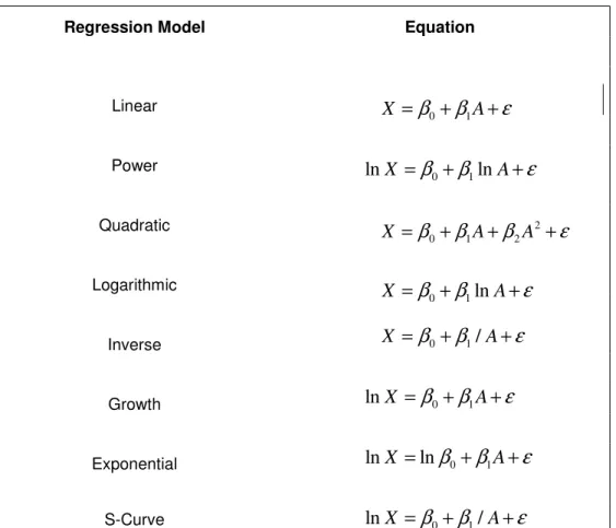
3.2 Commonly used Sales Response Functions

These models include linear, power, quadratic, logarithmic, inverse, growth, exponential or S shaped curves. Depending on the nature of the data, curve estimation and time series analyses methods are used to figure out the regression model that captures the effects of the explanatory (endogenous) variables on the sales variable in a most effective way. In order to establish the

(37)

relation between the advertising expenditures and sales, several regression models have been proposed.

Significance of the overall model, significance of the endogenous variables in the model, the coefficient of determinationR2, are considered as the performance criteria of the regression model.

Let X denote the sales quantity of a product, A be the amount spent for advertising, and

β

_i, i = 0, 1 are the parameters of the model. Error terms

ε

represent the unpredicted or unexplained variation in the response variable. Distribution of the error terms has great importance for the validation of the model. They are usually assumed to be independently and identically distributed normal random variables with mean µ and variance 2

σ (iid Normal (0,σ2).

(38)

Regression Model Equation Linear Power Quadratic Logarithmic Inverse Growth Exponential S-Curve

Table 1: Commonly used regression models

/A+

ε

(39)

Holthausen and Assmus [8] developed a model where there are n segments, and sales Y_i for segment i is expressed by an exponential function of advertising expenditure.

(1 exp( ))

i i i i

Y =B − −C A

i

B is called the market potential, or saturation level of the demand and C_i is the rate at which demand approaches market potential in response to advertising effortA_i. There are n different sales functions to be estimated independently; however, there exist covariance between the sales of different segments. They have chosen Seemingly Unrelated Regressions Model (SURM) to exploit correlations across regression equations.

Doyle and Saunders [7] developed a sales response function for multiproduct advertising budgeting. In their case they had a class of m merchandise (m=1,...,M), and n different types of advertising campaign.

Store wide sales due to advertising in period t is expressed by

1 1 ( ) M N t mn nt t m n S f A u = = =

∑∑

+ nt

A is the advertising expenditure on campaign naimed at the merchandiser class (n=m ). f_mnis a unique function relating advertising on campaign n to sales of merchandise m, and u_tis the random disturbance term.

Considering empirical findings for advertising from past researches they transformed their model to meet these assumptions and introduced lag relations into the model.

(40)

,

ln(1 )

mt m mni n t i mt

n i

S =a +

∑∑

b +A ₋ +u where i is the subscript identifying the lag terms, i = 0, 1,….., I. , a_mand b_mni are the parameters of the regression model.

They used data from a European variety store chain. From cross correlation analyses, they found the current and lagged advertising terms significant. Seasonal and cyclical terms were added to reflect the observed pattern in the data. 13 3 , 2 2 [ ln(1 )] mt m mni mni n t i mj jt mk kt mt n i j k S a w b A ₋ L l Y y u = = = +

∑∑

+ +

∑

+

∑

+

Using Lagrangian multipliers for the constrained advertising budget, and derivating the sales response function with respect to A_ntgave the optimum advertising expenditure values. After allocation, they concluded that without changing the advertising budget, profits could be increased up to 40 percent.

Conclusively, depending on the variety and the importance of the marketing variables, sales response functions can take many forms. After the statistical analyses, the variables that have the most explanatory power on the response variable can be used; hence a better prediction for the demand can be obtained.

3.3 An Application on Coffee Sales

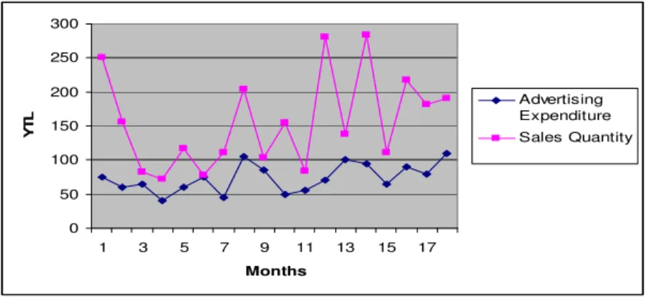
As an example, we present a sales response model for a major food production company in Turkey. We collected the sales data and related television, printed media and outdoor advertising expenditures for a soluble coffee for the years 2002-2003 as given in Table 2, Appendix A. In Figure 1, we plot the sales for 24 months.

(41)

25,8 26 26,2 26,4 26,6 26,8 27 27,2 27,4 27,6 27,8 Ja n-02 Mar .02 May .02 July -02 Sep -02 Nov -02 Ja n-03 Mar .03 May .03 July -03 Sep -03 Nov -03

Figure 1: Coffee Sales in Natural Logaritm from January 2002 to December 2003

We include the first and the second lags of the advertising expenditures in the regression analyses. Let S denote the coffee sales , TV be the amount spent for television, P be the amount for printed media, and O be the amount for outdoor advertising expenditures, t represents the months, and

β

_i, i = 0, 1, 2, 3 are the parameters of the model. Error terms

ε

represent the unpredicted or unexplained variation in the response variable.

Using the SPSS software, we found that the power model gives the best estimates among the regression models we mentioned in 3.2. Using backward elimination method we obtain the following regression model.

0 1 1 2 1 3

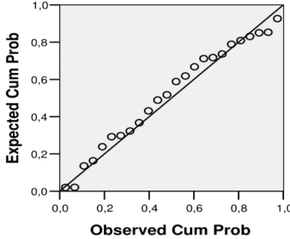
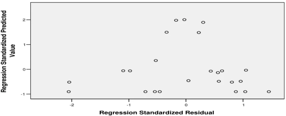
expenditures. Durbin Watson Test gives us a value 2,453 from which we can conclude that the error terms are not autocorrelated. The error variance is found out to be 0.073 (Table 3, Appendix A). The normal probability plot (Figure 2) and the standardized predicted values versus standardized residuals scatter plot (Figure 3) show that the error terms are independently and identically distributed normal random variables with mean zero and variance 0.073. Further information regarding the interpretation of such statistics is also provided in Chapter 5. 1,0 0,8 0,6 0,4 0,2 0,0

Observed Cum Prob

1,0 0,8 0,6 0,4 0,2 0,0 E xp ec te d C u m P ro b

Figure 2: Normal Probability Plot of Error Terms

The values are clustered around the straight line; hence the distribution of error terms matches the normal distribution.

(43)

1 0

-1 -2

Regression Standardized Residual

2 1 0 -1 R eg re ss io n St an da rd iz ed P re di ct ed Va lu e

Figure 3: Standardized predicted values versus standardized residuals Scatter Plot

The scatter plot does not show extreme fluctuations; therefore, we can assume that the error terms have the same variance 0.073.

The parameters of the model

β

_i’s i = 0, 1, 2, 3 are found to be 26.992, 0.006, 0.013, and 0.003 respectively (Table 4, Appendix A). We can consider

0

exp(

β

) as the baseline sales when the advertising expenditures are zero. Other parameters of the model

β

_i i=1, 2,3 can be interpreted as the ratio of the sales value for a unit increase in advertising expenditures. For example, when we increase the TV advertising expenditure 1 unit, the ratio of

1 and

t t

S₊ S is equal to exp (0.013) which is equal to 1.013085.

The sales response function for the coffee example has lagged terms for the television and printed media advertising variables; moreover, we could not obtain the exact values for the price of the product, production, holding, and lost sales costs for our single period newsboy problem. Therefore, we chose

(44)

not to integrate coffee sales response model into our newsboy setting. Instead we conduct our numerical example for the data set acquired from Holthausen and Assmuss [8].

(45)

C h a p t e r 4

SIMULTANEOUS DECISION

MODEL FOR PRODUCTION

AND ADVERTISING

In this chapter, we introduce our model that incorporates sale response functions to a single period newsboy problem in order to determine the optimal production quantity and advertisement expenditure under a budget constraint.

4.1 The Single Period Newsboy Problem

The newsboy problem is a stochastic inventory replenishment problem. For a known distribution for demand, it seeks the optimal quantity to be ordered before the actual demand is observed. The problem expresses the firm’s profit function in terms of revenue and the cost components. A fixed ordering cost cQis paid to order Q units of products. Firm markets the product for p monetary units. When the ordered quantity is greater than the realized demand the firm sells as many products as its demand and a holding cost of h per unit is incurred for the unsold products. On the other hand, when the demand exceeds the ordered quantity the firm would sell all of the products but will be subject to a lost sales cost ofλ per unit of unsatisfied demand.

(46)

Considering whether the demand is greater or smaller than the ordered quantity, the profit function takes the following forms.

Let x be the demand,

∂ = = − − + + +

∂ , i.e., Q* satisfies the equation

( ) p c F Q p h

λ

− − = + +

In this study, we consider a company whose objective is to find the optimal production quantity Q, and the optimal advertising expenditure with the integration of the demand response function in to the newsboy problem to maximize its expected profit for different budget constraints.

(47)

Similarly, x representing the demand, and A is the advertising expenditure, we can express the profit function of our setting as follows:

( , ) ( ) ( ) P Q A px h Q x cQ A x Q pQ cQ A x Q pQ

λ

x Q cQ A x Q = − − − − ≤ = − − = = − − − − >

4.2 Integration of the Demand Response Function into the Newsboy Problem

In this section, we analyze the integration of linear and power demand response functions into the newsboy problem. By the integration of the demand response function, the new newsboy problem will be transformed into a profit equation which not only seeks for the optimal quantity to produce, but also for the optimal advertising expenditure to maximize the expected profit.

4.2.1 Linear Demand Response Function

Let A be the advertising expenditure for a product for a single period. In general we express the sales quantity X as X = f h A( ( ), )

ε

where h A( ) is a known function of the advertising budget that links the sales to the advertising expenditure A and

ε

is a random term.

In linear response model the sales is expressed as

( ( ), )

(48)

where

β

₀ and

β

₁ are the parameters of the linear model.

= ≤ = + ≤ ≤ − Φ

Φ on function of a standart normal random variable.

We can now write the expected profit function including the advertising expenditure as a cost component by incorporating the sales distribution given in (2) into the expected profit function given in (1).

0 0 0 0 [ ( , )] [ ( ) ( )] [ ( ) ( )] [ ( ) ( )] (1 ( )) ( ( )) (1 ( )) ( ) ( ) ( ) Q Q Q Q Q Q Q E P Q A p Q dF x xdF x h Q dF x xdF x xdF x Q dF x cQ A pQ F Q hQ F Q Q F Q cQ A p h xdF x xdF x λ λ λ ∞ ∞ ∞ = + − − − − − − = − − + − − − + + −