Pressure Control of Cold Air Testing Plant with Delay
Resistant Closed-loop Reference Model Adaptive
Control
Anil Alan
∗and Yildiray Yildiz
† Bilkent University, Cankaya, Ankara, 06800, TurkeyUmit Poyraz
‡Roketsan Missiles Inc., Elmadag, Ankara, 06780, Turkey
This paper deals with the control problem of obtaining desired gas pressure inside a control volume with constant inlet mass flow rate of cold air. Cold air flow system dynamics is similar to that of a gas generator of a throttleable ducted rocket, which sends fuel in gaseous form, with metal additives, to ram combuster with desired amount of mass flow rate to obtain variable thrust. Being able to control gas pressure in cold air flow system is a milestone towards obtaining a fully developed throttleable ducted rocket gas generator controller. In this study, a detailed modeling of the cold air test plant together with a delay resistant closed-loop reference model adaptive controller design is presented. The proposed controller is compared with several other alternatives including a classical proportional-integral controller, model reference adaptive controller and a closed-loop reference model adaptive controller that does not have explicit delay compensation. Simulation results verifying the performance improvement of the delay resistant controller over the alternatives are presented.
Keywords: cold air testing plant, throttleable ducted rockets (TDR), pressure control, closed-loop reference model (CRM), model reference adaptive control (MRAC), time delay resistant
I.
Introduction
A throttleable ducted rocket (TDR) has the ability to adjust its speed during flight by controlling the fuel mass flow rate. This technique helps TDRs make maneuvers and find their moving targets more efficiently during flight, compared to their counterparts. In TDRs, the gas generator (GG) provides the variable fuel mass flow rates to the ram combuster (RC), where variable thrust is generated. GG contains oxidizer deficient solid propellant, which is ignited initially to generate fuel in gaseous form that flows to the RC for further combustion due to the high pressure in the GG.1
It is shown in earlier studies1–11 that with the precise control of the pressure inside the GG, demanded
thrust profile for the missile can be achieved. The desired GG pressure is obtained by manipulating the throat area between the GG and the RC using an active valve system. In our earlier work, we proposed employing adaptive control for the GG pressure control,12 where experimental results were provided to demonstrate
performance improvements over widely used classical control methods. In this study, we employ a delay-resistant adaptive controller, where the uncertainties are addressed by adaptation together with explicit delay compensation required to handle large system delays. Specifically, in this study, we develop a nonlinear cold air flow system model, by using open loop experimental tests, to obtain a high fidelity simulation testing bed that can be utilized for comparatively evaluating several controller approaches. Then, we design a proportional integral (PI) controller using linearized plant dynamics based on predefined performance criteria. It is observed from simulations that the performance of the PI controller reduces as operating
∗Graduate student, Mechanical Engineering Department.
†Assistant Professor, Mechanical Engineering Department.
‡Senior Propulsion Systems Design Engineer, Propulsion Systems.
Downloaded by BILKENT UNIVERSITY on August 6, 2018 | http://arc.aiaa.org | DOI: 10.2514/6.2017-0121
55th AIAA Aerospace Sciences Meeting 9 - 13 January 2017, Grapevine, Texas
10.2514/6.2017-0121 AIAA SciTech Forum
point moves away from the equilibrium point used for linearization. In order to tackle this problem, we design a model reference adaptive controller (MRAC) that can handle plant parameter variations at different operating points. It is shown via simulations that although MRAC is successful at controlling the plant with a reasonable transient response, it fails to provide an acceptable performance for more demanding reference pressure variations. A Closed-loop Reference Model (CRM) modification13 is then added to the MRAC by
feeding back the tracking error to the reference model, which is shown in the literature to damp oscillations due to high adaptation gains. In our simulations, CRM is observed to give smoother controller parameter signals by reducing down the norm of tracking error between the plant and the reference model outputs. However, it is observed that the CRM modification is still not enough to obtain acceptable system response for highly demanding reference trajectories, due to the relatively large input time delay in the experimental system. To obtain a reasonable performance, we add explicit delay compensation to CRM adaptive controller, which is novel in the literature. Proposed controller provided dramatically better tracking results compared to the alternatives.
Modeling of physical system is given in Section II. Details about controller design are provided in Section III. Numerical simulation results are given in Section IV. Finally a summary of paper is provided in Section V.
II.
Plant Model
A. Cold Air Testing Plant
CONTROL VOLUME
Air flow inlet
Pressure regulator Nitrogen source Pressure sensors BLDC motor Spindle Pintle
Actuator & valve mechanism
Air flow outlet
Throat with variable open throat area
Figure 1: Schematic of Cold Air Testing Plant (CATP)
A schematic of the Cold Air Testing Plant (CATP) is presented in Figure 1. It is assumed that the gas (nitrogen) inside the control volume satisfies the ideal gas condition. The difference between the mass flow rates going into the control volume, ˙min, and going out of the control volume, ˙mout, is given as
˙
min− ˙mout=
˙ P V
RT (1)
where R is the specific gas constant and T and V are the temperature and volume of the gas in the control volume. It is assumed that ˙minis kept constant by utilizing a pressure regulator. It is noted that the process
is assumed to be isothermal with no change in the control volume, hence ˙V = ˙T = 0.
Mass flow coming out of the control volume is a function of throat area (At) and pressure inside the
control volume (P ). Assuming chocked flow conditions at the exit throat, it is obtained that, ˙ mout= P At(( 2 γ + 1) (γ−1γ )) r γ RT∗ = P At c∗ (2)
where γ is the specific heat ratio of air, T∗ is the temperature at the throat and c∗ is the characteristic velocity of the gas inside the control volume. Using (1) and (2), it is obtained that
˙
P = c1m˙in− c2P At= M − c2P At (3)
where c1 = RTV , c2= cc1∗ and M = c1m˙in. It is noted that the throat area, At, is the control input for the
plant.
Linearizing the dynamics around the equilibrium point P = P0and At= At0, we obtain that,
˙
P = ∆ ˙P = (−c2At,0)∆P − (c2P0)∆At (4)
where ∆P = P − P0 and ∆At = At− At,0 are the derivations from the equilibrium points. Defining
ap≡ c2At,0 and bp≡ −c2P0, (4) can be rewritten as
∆ ˙P = −ap∆P + bp∆At. (5)
Equation (5) shows that the plant dynamics are highly dependent on the operation point (P0 and At0)
where the DC gain is k = −P0
At0 and the plant pole is determined as −c2At,0.
We choose three different operating points, given in Table 1, and analyze system dynamics at these points. While calculating corresponding throat area values for given pressure values at steady state using (3), a constant air mass flow rate is used, corresponding to c1m = M . M is obtained from open loop tests˙
of testing bed. Bode plots of linearized plant dynamics at trim points are given in Figure 2. Table 1: Trim points
Trim points First trim point Second trim point Third trim point
Pressure (normalized) P1 P2 P3 Throat Area (mm2) A t,1 At,2 At,3 bp -8,176 -12,264 -16,35 ap (pole position) -17 -11,33 -8,5 Time constants (ms) 59 89 118 -60 -40 -20 0 20 Magnitude (dB) 10-1 100 101 102 103 90 135 180 Phase (deg)
First Trim Point Second Trim Point Third Trim Point
Frequency (rad/s)
Figure 2: Bode plots of trim points
B. Actuator Dynamics
CATP pressure is manipulated by changing the exit throat area. Here, a brushless DC motor (BLDC motor) is used as the actuator, with a valve mechanism to vary the throat area, At.
The BLDC motor used in the experimental setup, which is manufactured by Maxon Motor Company, is an EC-max 30, 60 Watt, 24 Volt motor with a driver card EPOS2 70/10. This motor together with its driver is modeled as a first order system whose time constant is calculated to be 30 ms, which is considered as small compared to the time constants of the CATP. Therefore, we ignore the actuator dynamics during the controller design and only consider dominant CATP dynamics. It is noted that linearizing system dynamics and ignoring actuator dynamics are used to simplify the controller design, and full nonlinear plant dynamics together with actuator dynamics are employed during simulation studies.
C. Valve Geometry
In this subsection, we present the relationship between the actuation provided by the BLDC motor and the throat area, At. The valve mechanism includes a spindle to convert the rotational motion of the motor into
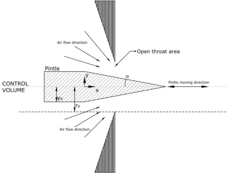
the translational motion of a pintle at the throat. Detailed 2D drawing of the valve is given in Figure 3.
Open throat area
Pintle moving direction
α r0 y0 x y Pintle CONTROL VOLUME
Air flow direction
Air flow direction
Figure 3: Valve
There is a circular opening at the exit with a constant throat area. The pintle has a degree of freedom in x direction and due to its conical surface (depicted as a triangle in 2D drawing), open throat area changes as the pintle moves along the x axis. The cylindrical part at the back of the pintle, whose cross sectional area is smaller than the fixed throat area, makes sure that the open throat area Atis always nonzero, protecting
the system from rapid pressure build up.
The relationship between the movement of the pintle in the x direction and closing of the throat in the y direction is given as
y = y0− tan(α)x (6)
where each variable and constant are shown in Figure 3. The open throat area is calculated as, At= (r20− y
2)π. (7)
Also, using the gear box (1:14) and the spindle (2 mm per rotation) parameter values, following equation between angular position of the DC motor rotor (θ) and linear position of the pintle (x) is obtained as,
x = θ
28000 (8)
where the unit of θ is quadrature (4000 quadrature (qc) correspond to 1 rotation (or 2π rad)) while x has an unit of mm. Using (6-8), we obtain
At[mm2] = (v0+ v1θ + v2θ2)π. (9)
For the specific valve geometry parameters (r0, y0, α) used in the experimental system, it is demonstrated in
Fig. 4 that (9) shows almost linear relationship in the selected operation range (since v2<< v1). Therefore,
in the developed plant model, it is assumed that relationship between output of the BLDC motor (rotational position θ) and control input of the CATP system (At) is linear, by ignoring v2.
0 0.5 1 1.5 2 2.5 3 3.5 4 4.5
Angular Position of BLDC Motor (qc) #105 0 0.2 0.4 0.6 0.8 1
Open Throat Area (normalized)
Figure 4: Relationship between BLDC output (θ) and controller input (At)
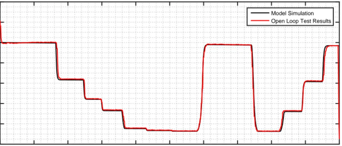
10 15 20 25 30 35 40 45 50 55 60 Time(sec) 0 0.2 0.4 0.6 0.8 1 1.2 1.4 Pressure (normalized) Model Simulation Open Loop Test Results
Figure 5: Open loop test results and model outputs
Finally, an input time delay of 300ms, on average, due to communication and computation processes that is observed in real-time test system is included in the plant model. Figure 5 shows the comparison between the open loop test and simulation results of the plant. A reasonably close match is realized.
III.
Controller Design
A. Proportional-Integral (PI) Controller
The closed loop system performance specifications used for the design of the proportional integral (PI) controller is given in Table 2.
Table 2: Specifications of closed loop dynamics
Steady state error Minimum rise time Maximum settling time (5 %) Maximum overshoot
0 % 0.6 sec 1.5 sec 10 %
Using the following PI controller,
GP I = kp+
kI
s (10)
the closed loop transfer function is obtained as GCL=
bp(kps + kI)
s2+ (a
p+ kpbp)s + kIbp
(11) where ap and bp are the parameters of the open loop system (5). It is noted that the input delay is ignored
in this controller design.
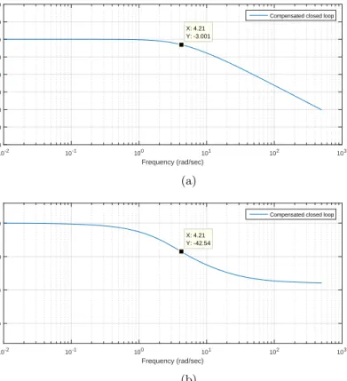
Using the second trim point (see Table 1), the gains of the PI controller are calculated as kI = −10 and
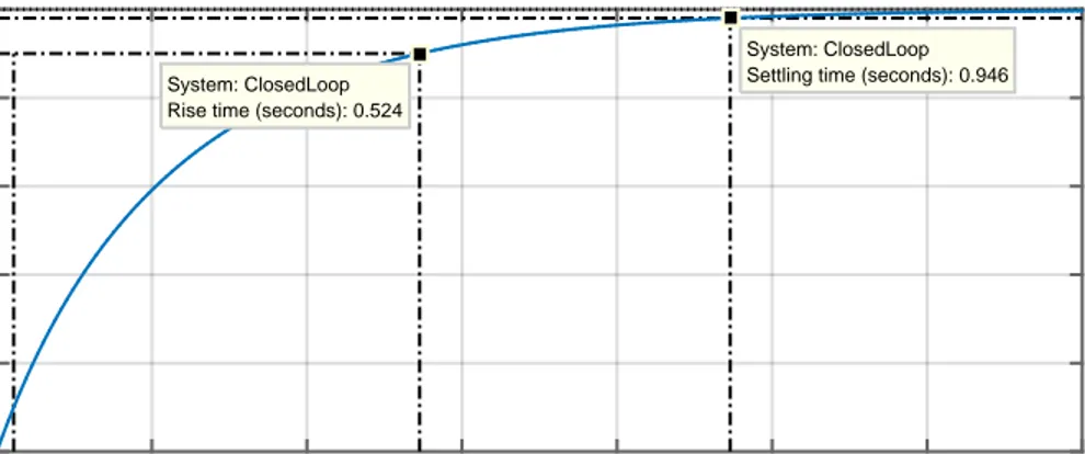
kP = −0, 4. The bode plot and the step response of the compensated system are provided in Fig. 6 and Fig.
7, respectively. 10-2 10-1 100 101 102 103 Frequency (rad/sec) -60 -50 -40 -30 -20 -10 0 10 20 Magnitude (dB)
Compensated closed loop X: 4.21 Y: -3.001 (a) 10-2 10-1 100 101 102 103 Frequency (rad/sec) -150 -100 -50 0 Phase (deg)
Compensated closed loop
X: 4.21 Y: -42.54
(b)
Figure 6: Bode plot of the compensated closed loop system with PI controller (a) magnitude and (b) phase
B. Model Reference Adaptive Controller (MRAC) Consider the first order plant dynamics
˙
x(t) = −apx(t) + bpu(t) + d (12)
where ap and bp are the plant parameters from linearization, and x and u are the pressure and the open
throat area deviations from the equilibrium point (∆P and ∆At), respectively. d is the disturbance acting
on the system dynamics.
0 0.2 0.4 0.6 0.8 1 1.2 1.4 0 0.2 0.4 0.6 0.8 1 Time (seconds) Amplitude System: ClosedLoop Settling time (seconds): 0.946 System: ClosedLoop
Rise time (seconds): 0.524
Figure 7: Step response of the compensated plant with PI controller
To compensate the uncertainties in the linearized plant dynamics (5), the following adaptive controller structure is used
u = k1+ k2x + k3r. (13)
The reference model is given as
˙
ym= −amym+ bmr (14)
where am> 0 and bm= am for unity DC gain.
It can be shown that the following adaptation laws result in a stable closed loop system where all the signals are bounded and the tracking error e = x − ymconverges to zero:
˙ k1= γ1e(t) (15) ˙ k2= γ2x(t)e(t) (16) ˙ k3= γ3r(t)e(t) (17)
where γ1, γ2, γ3are positive scalars representing the adaptation rates. During the implementation, a
projec-tion algorithm14is used to prevent the parameter drift due to unmodeled dynamics and noise.
Tuning of adaptation gains (γ’s) are done using formula the15
γi=
|ki,0|
3τm(r∗)2
(18) for i = 1, 2, 3 where τmis the time constant of the reference model and r∗ is the characteristic value of the
reference signal. ki,0values are the initial conditions of the controller parameters found from ideal conditions
that are computed using known plant parameters from Table 1. Note that k1,0is optimized using simulation
trials.
C. Closed-Loop Reference Model (CRM) Modification
To improve the transient response of the system, we apply the closed-loop reference model (CRM) modifi-cation12, 13to the adaptive controller designed in the previous section.
Modified reference model is given as ˙
ym(t) = −amym(t) + bmr(t) − l(x(t) − ym(t)) (19)
where am= bm> 0 and l < 0 is called the CRM gain and provides another free design parameter to obtain
improved transient response. By using CRM, we are able to increase adaptation rates, which otherwise would result in oscillatory convergence of the controller parameters.
D. Delay Resistant CRM (DR-CRM)
In the controller designs presented so far, the input time delay is ignored. In this section, we introduce another modification to the adaptive controller, which explicitly compensate the time delay. We name the resultant controller the delay resistant closed-loop reference model (DR-CRM) adaptive controller. It is noted that the delay compensation proposed here were used earlier by the author Yildiz in open loop model reference adaptive controllers where the resulting controller was shown to perform dramatically better compared to existing approaches.16 For the other delay compensating adaptive approaches, see Ref. 17.
With the input time delay the plant dynamics is expressed as ˙
x(t) = −apx(t) + bpu(t − τ ) + d (20)
where ap and bp are the plant parameters from linearization, and x and u are the pressure and the open
throat area deviations from the equilibrium point (∆P and ∆At), respectively. τ is the known input delay
and d is the disturbance acting on the system dynamics. The reference model for the TD-CRM is given ˙
ym(t) = −amym(t) + bmr(t − τ ). (21)
Baseline controller structure is given as
u(t) = k1+ k2x(t + τ ) + k3r(t) (22)
which results in the closed loop dynamics ˙
x(t) = (−ap+ k2bp)x(t) + bpk3r(t − τ ) + d + bpk1. (23)
It can be shown that there exist controller parameters k∗1, k2∗, k3∗ which make the closed loop dynamics ˙
x(t) = −amx(t) + bmr(t − τ ) (24)
which is same as the reference model dynamics given in (21). However, x(t + τ ) term is non-casual, and we need ”positively forecast (posicast)” method first proposed by Smith18and later developed by Manitius and Olbrot19 to deal with this problem. Manitius and Olbrot introduce Finite Spectrum Assignment to make x(t + τ ) term casual using finite time integrals.
x(t + τ ) = e−apτx(t) +
Z 0
−τ
eapηu(t + η)dη (25)
For the software implementation purposes, the integral term in (25) needs to be approximated as Z 0 −τ eaηu(t + η)dη = m X i=1 ea(−dt∗i)u(t − dt ∗ i) (26)
for m = dtτ where dt is the sampling interval, τ is the input time delay and a is the pole location of the first order plant. Defining the vector of coefficient terms for the integral approximation as
λi= ea(−dt∗i) (27)
and delayed input term vector as,
¯
ui= u(t − dt ∗ i) (28)
for i = 1 . . .dtτ, the control input (25) can be rewritten as
u(t) = k1+ k2(λ0x(t) + ¯λTu) + k¯ 3r(t) (29)
where λ0= e−aτ.
Analysis up to here shows that for known plant parameters ap and bpand disturbance d, it is possible to
design a delay resistant controller. Now, it can be shown that adaptive laws in equations (15-17) along with
˙λ(t) = Γe1(t)¯u (30)
keeps the system stable with tracking error converging to zero in case of unknown plant parameters and constant disturbance. Γ is a diagonal adaptation rate matrix whose elements are positive. e1= x − ym is
the tracking error between plant output and delayed reference model.
We proceed to add CRM modification to delay resistance control to have smoother transient signals. Modified reference model is given as
˙
ym(t) = −amym(t) + bmr(t − τ ) − l(x(t − τ ) − ym(t − τ )) (31)
IV.
Simulations
In this section, classical, adaptive and delay resistant controller performances are compared using simula-tions. Simulations are conducted using full nonlinear plant dynamics developed in earlier sections including actuator dynamics. The parameter values used in the plant model are not given here due to classified infor-mation. Please note that the pressure and throat area values are normalized due to same reason. Simulink toolbox of Matlab R is used for numerical simulations with a fixed step size of 50 ms.
20 25 30 35 40 45 50 55 60 65 70 75 Time (sec) 0.3 0.4 0.5 0.6 0.7 0.8 0.9 1 1.1 1.2 1.3 Pressure (normalized) Reference command PI MRAC
Figure 8: Tracking curves for the PI controller and MRAC at 3 different operating points.
20 30 40 50 60 70 Time (sec) 0.2 0.4 0.6 0.8 1 1.2 1.4 1.6 Pressure (normalized) MRAC CRM Reference command Delay resistant CRM
Figure 9: Tracking curves for MRAC, CRM and TD-CRM with more demanding reference trajectories. In Fig. 8 simulation results are given demonstrating the performances of the model reference adaptive control (MRAC) and proportional integral (PI) controller. We did not include results of closed-loop reference model (CRM) adaptive controller and delay resistant CRM (DR-CRM) in this figure, but they are very close to the MRAC results. Although PI controller is able to provide the desired performance around 15 bar, it can not sustain this for different operation points. When plant is operated at high pressures, PI controller has oscillatory response, while it gives slow reaction to low pressures. On the other hand, MRAC can adapt itself to changing operating conditions.
CRM and delay compensation modifications did not show considerable performance improvements for
20 30 40 50 60 70 Time (sec) -0.2 0 0.2 0.4 0.6 0.8 1 1.2
Throat Area (normalized)
MRAC CRM Delay resistant CRM
Figure 10: Control signals for MRAC, CRM and TD-CRM.
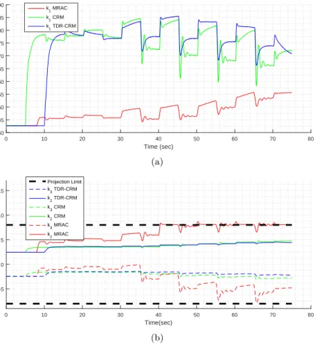
0 10 20 30 40 50 60 70 80 Time (sec) 140 145 150 155 160 165 170 175 180 185 190 k 1 MRAC k1 CRM k1 TDR-CRM (a) 0 10 20 30 40 50 60 70 80 Time(sec) -5 0 5 10 15 Projection Limit k3 TDR-CRM k2 TDR-CRM k3 CRM k2 CRM k3 MRAC k2 MRAC (b)
Figure 11: Controller parameters (a) k1 and (b) k2 and k3 along with projection boundaries for MRAC,
CRM and TD-CRM.
the desired references presented in Fig. 8. To demonstrate the difference that these modifications can make, more demanding reference trajectories were tested together with new reference models with faster dynamics, which would speed up the closed loop response of the system. The results of these simulations are given in Figure 9-11. As seen from these results, MRAC response is oscillatory for high pressure variations. Although CRM damps most of the oscillations, it still has undesired amount of overshoot at high pressures. DR-CRM has some overshoot, but it is within the specifications. Furthermore, DR-CRM is able to make the plant
reach its steady state value at low pressures at a faster rate and demonstrates a smooth tracking response. In Fig. 11, the variations of adaptive control parameters are seen together with the effect of the projection algorithm. It is observed that MRAC parameters hit the projection boundaries much faster than the CRM and DR-CRM parameters.
V.
Summary
In this paper, the modeling and control of a cold air testing plant are presented. It is demonstrated that the model reference adaptive controller shows a better performance at various operating points compared to a classical proportional integral controller. Furthermore, it is shown that when the reference trajectories become more demanding, model reference adaptive controller provides an oscillatory response and closed-loop reference modification improves the performance of the adaptive controller by damping some of the oscillations. However, it is demonstrated that the best performance can be obtained by the proposed delay-resistant closed loop reference model adaptive controller.
References
1P. Pinto and G. Kurth, “Robust propulsion control in all flight stages of a throtteable ducted rocket,” in Proc.
AIAA/ASME/ASEE Joint Propulsion Conference & Exhibit, no. AIAA-2011-5611, (San Diego, California), pp. 1–12, 2011.
2A. G. Sreeriatha and N. Bhardwaj, “Mach number control-ler for a flight vehicle with ramjet propulsion,” in Proc.
AIAA/ASME/SAE/ASEE 35th Joint Propulsion Conference and Exhibit, no. AIAA 99-294, (Los Angeles, CA), 1999.
3J. Chang, B. Li, W. Bao, W. Niu, and D. Yu, “Thrust control system design of ducted rockets,” Acta Astronautica,
vol. 69, no. 1, pp. 86–95, 2011.
4C. Bauer, N. Hopfe, P. Caldas-Pinto, F. Davenne, and G. Kurth, “Advanced flight performance evaluation methods
of supersonic air- breathing propulsion system by a highly integrated model based approach,” in Proc. RTO-MP-AVT-208, pp. 1–14, 2012.
5C. Bauer, F. Davenne, N. Hopfe, and G. Kurthy, “Modeling of a throttleable ducted rocket propulsion system,” in Proc.
AIAA/ASME/ASEE Joint Propulsion Conference & Exhibit, (San Diego, California), pp. 1–15, 2011.
6S. M. W. Miller and W. Burkes, “Design approaches for variable flow ducted rockets,” in Proc. AIAA/SAE/ASME 17th
Joint Propulsion Conference, (Colorado Springs, Colorado), 1981.
7J. L. Bergmans and R. D. Salvo, “Solid rocket motor control: theoretical motivation and experimental demonstration,”
in Proc. AIAA/ASME/SAE/ASEE 39th Joint Propulsion Conference and Exhibit, pp. 20–23, 2003.
8S. Joner and I. Quinquis, “Control of an exoatmospheric kill vehicle with a solid propulsion attitude control system,” in
AIAA Guidance, Navigation, and Control Conference and Exhibit, no. AIAA 2006-6572, (Keystone, Colorado), 2006.
9W. Lee, Y. Eun, H. Bang, and H. Lee, “Efficient thrust distribution with adaptive pressure control for multinozzle solid
propulsion system,” Journal of Propulsion and Power, vol. 29, no. 6, pp. 1410–1419, 2013.
10J. L. Bergmans and R. I. Myers, “Throttle valves for air tur-bo-rocket engine control,” in Proc. AIAA/ASME/SAE/ASEE
33th Joint Propulsion Conference and Exhibit, 1997.
11C. A. Davis and A. B. Gerards, “Variable thrust solid propulsion control using labview,” in Proc.
AIAA/ASME/SAE/ASEE 39th Joint Propulsion Conference and Exhibit, no. AIAA 2003-5241, (Huntsville, Alabama), 2003.
12U. P. Anil Alan, Yildiray Yildiz and U. Olgun, “Gas generator pressure control in throttleable ducted rockets: A classical
and adaptive control approach,” in Propulsion and Energy Forum, 51st AIAA/SAE/ASEE Joint Propulsion Conference, no. AIAA 2015-4236, (Orlando, FL), 2015.
13T. E. Gibson, Closed-Loop Reference Model Adaptive Control: with Application to Very Flexible Aircraft. Phd thesis,
MASSACHUSETTS INSTITUTE OF TECHNOLOGY, 2014.
14J.-B. Pomet and L. Praly, “Adaptive nonlinear regulation: Estimation from the lyapunov equation,” IEEE
TRANSAC-TIONS ON AUTOMATIC CONTROL, vol. 37, pp. 729–740, June 1992.
15Y. Yildiz, A. Annaswamy, D. Yanakiev, and I. Kolmanovsky, “Spark ignition engine idle speed control: An adaptive
control approach,” IEEE Transactions On Control Systems Technology, vol. 19, no. 5, pp. 990–1002, 2011.
16Y. Yildiz, A. Annaswamy, I. Kolmanovsky, and D. Yanakiev, “Adaptive posicast controller for time-delay systems with
relative degree n∗≤ 2,” Automatica, vol. 46, no. 2, pp. 279–289, 2010.
17M. Krstic, Delay Compensation for Nonlinear, Adaptive, and PDE Systems. Boston: Birkhauser, 2009.
18O. J. Smith, “A controller to overcome dead time,” ISA Journal, vol. 6, 1959.
19A. Z. Manitius and A. W. Olbrot, “Finite spectrum assignement problem for systems with delays,” IEEE Transactions
on Automatic Control, vol. 24, no. 4, 1979.