Interactive Training of Advanced Classifiers for
Mining Remote Sensing Image Archives
Selim Aksoy
Bilkent University
Department of Computer Engineering Bilkent, 06800, Ankara, Turkey
[email protected]
Krzysztof Koperski, Carsten Tusk,
Giovanni Marchisio
Insightful Corporation 1700 Westlake Ave. N., Suite 500
Seattle, WA, 98109, USA
{
krisk,ctusk,giovanni
}@insightful.com
ABSTRACT
Advances in satellite technology and availability of down-loaded images constantly increase the sizes of remote sensing image archives. Automatic content extraction, classification and content-based retrieval have become highly desired goals for the development of intelligent remote sensing databases. The common approach for mining these databases uses rules created by analysts. However, incorporating GIS informa-tion and human expert knowledge with digital image pro-cessing improves remote sensing image analysis. We devel-oped a system that uses decision tree classifiers for inter-active learning of land cover models and mining of image archives. Decision trees provide a promising solution for this problem because they can operate on both numerical (con-tinuous) and categorical (discrete) data sources, and they do not require any assumptions about neither the distri-butions nor the independence of attribute values. This is especially important for the fusion of measurements from different sources like spectral data, DEM data and other ancillary GIS data. Furthermore, using surrogate splits pro-vides the capability of dealing with missing data during both training and classification, and enables handling instrument malfunctions or the cases where one or more measurements do not exist for some locations. Quantitative and qualitative performance evaluation showed that decision trees provide powerful tools for modeling both pixel and region contents of images and mining of remote sensing image archives. Categories and Subject Descriptors: I.5.2 [Pattern Recog-nition]: Design Methodology; I.4.8 [Image Processing and Computer Vision]: Scene Analysis
General Terms: Algorithms, Design, Experimentation Keywords: Decision tree classifiers, missing data, data fu-sion, remote sensing, land cover analysis
Permission to make digital or hard copies of all or part of this work for personal or classroom use is granted without fee provided that copies are not made or distributed for profit or commercial advantage and that copies bear this notice and the full citation on the first page. To copy otherwise, to republish, to post on servers or to redistribute to lists, requires prior specific permission and/or a fee.
KDD’04, August 22–25, 2004, Seattle, Washington, USA.
Copyright 2004 ACM 1-58113-888-1/04/0008 ...$5.00.
1.
INTRODUCTION
Remotely sensed imagery has become an invaluable tool for scientists, governments, military and the general public to understand the world and its surrounding environment. Military applications include using land cover classification to derive tactical decision aids like landing zone and troop movement plans, to manage ecosystems of military lands and waterways, and to study interactions between mission activities and ecological patterns. Similarly, land cover maps help civil users to perform land use monitoring and manage-ment, fire protection, site suitability, agricultural and public health studies.
The amount of data received from satellites is constantly increasing. For example, NASA’s Terra satellite sends more than 850GB of data to Earth every day [15]. Automatic content extraction, classification and content-based retrieval have become highly desired goals to develop intelligent re-mote sensing image databases. State-of-the-art rere-mote sens-ing image analysis systems aid users by providsens-ing classifica-tion tools that use spectral informaclassifica-tion or texture features as the input for statistical classifiers that are built using un-supervised or un-supervised algorithms. The most commonly used classifiers are the minimum distance classifier and the maximum likelihood classifier with a Gaussian density as-sumption. Spectral signatures and other features do not al-ways map conceptually similar patterns to nearby locations in the feature space and limit the success of minimum dis-tance classifiers. Furthermore, these features do not always have Gaussian distributions so maximum likelihood classi-fiers with this assumption fail to model the data adequately. Like any data analysis problem, domain knowledge and prior information is very useful in land cover classification. Incorporating supplemental GIS information and human ex-pert knowledge into digital image processing has long been acknowledged as a necessity for improving remote sensing image analysis [8]. Artificial intelligence research and devel-opments in rule-based classification systems have enabled a computer to mimic the heuristics and knowledge that a human expert uses in interpreting an image. Consequently, rule-based classification systems [10] have been successfully used for fusion of spectral and ancillary data in applications such as land cover classification [8, 11], land cover change monitoring [17], sea ice classification [18], and ridge line ex-traction from Digital Elevation Model (DEM) data [14].
However, a common problem in all of these attempts has been the translation of expert knowledge to a
computer-usable format. First, remotely sensed data are converted into formats supported by statistical analysis packages; then, these packages are used to create rules; finally, the rules are re-formatted so that they can be used in a rule-based im-age classifier [8, 11]. Today, commercial-of-the-shelf remote sensing image analysis systems have rule-based classification modules but they operate on individual scenes and require an expert to create the rules. This requirement for an enor-mous amount of manual processing even for small data sets makes knowledge discovery in large remote sensing archives practically impossible.
The VisiMine system [9] we have developed supports in-teractive classification and retrieval of remote sensing images by modeling them on pixel, region and scene levels. Pixel level characterization provides classification details for each pixel with regard to its spectral, textural and other ancil-lary attributes. Following a segmentation process, region level features describe properties shared by groups of pixels. Scene level features model the spatial relationships of the regions composing a scene using a visual grammar. This hierarchical scene modeling with a visual grammar aims to bridge the gap between features and semantic interpretation. This paper describes our work on developing decision tree-based tools to automate the process of acquiring knowledge for image analysis and mining in remote sensing archives. Decision tree classifiers are used to model image content in pixel and region levels. VisiMine provides an interactive en-vironment for training customized semantic land cover labels from a fusion of visual attributes. Spectral values, ancillary GIS layers and other image attributes like textural features are used in decision tree learning. The learning process also includes algorithms for handling missing data and automatic conversion of models into rule bases.
The rest of the paper is organized as follows. The system architecture and data used in the experiments is introduced in Section 2. The classifiers used for land cover modeling are described in Section 3. User interaction tools for train-ing and evaluattrain-ing these models are presented in Section 4. Performance evaluation for the proposed system is discussed in Section 5. Conclusions are given in Section 6.
2.
PROTOTYPE SYSTEM DESIGN
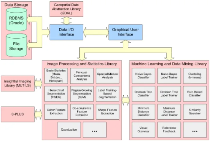
VisiMine system architecture is given in Figure 1. The image processing, statistics, machine learning and data min-ing libraries are implemented in C/C++. The graphical user interface is implemented in Java. Oracle is used as the RDBMS to store and access images, features and metadata. VisiMine also has a seamless interface with Insightful’s S-Plus statistical analysis software.
The input to the system is raw image and ancillary data. This data is automatically processed by unsupervised algo-rithms in the image processing library for feature extrac-tion. Original data and extracted features become the in-put to classification algorithms in the machine learning li-brary. The user interacts with the system by providing a list of land cover labels and corresponding training examples. Then, the machine learning library seamlessly transfers this expert knowledge into classification models in terms of de-cision trees and rules. Intuitive but powerful visualization tools allow the user examine the classification models and provide feedback to the system. These models can be used to classify other images in the same data set, or can be used to search other collections for similar scene structures.
Figure 1: VisiMine system architecture. The image processing library contains unsupervised algorithms to process both spectral and ancillary data to do feature extraction. The machine learning library contains automatic and semi-automatic algorithms to train higher-level class models. User can interact with the system to provide training examples and feedback to update the models.
2.1
Pixel Level Data
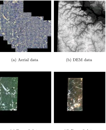
The image and ancillary raster data used for evaluating the system described in the paper consist of Aerial (1.8m resolution, 3 bands), Ikonos (4m resolution, 4 bands, 2 sets) and DEM (30m resolution, 1 band) data layers that cover the Fort A.P. Hill area in Virginia and are provided by the U.S. Army Topographic Engineering Center. These layers were upsampled to the same resolution (1.8m) where each band has 11, 683 × 11, 677 pixels.
We also extracted Gabor wavelet features [6, 13] for micro-texture analysis on the first band of Aerial data. (We also extracted Gabor features using the other Aerial and Ikonos bands but did not observe any significant improvement in the results.) Gabor features were computed by filtering an image with Gabor wavelet kernels at different scales and ori-entations. We used kernels rotated by nπ/8, n = 0, . . . , 7, at two scales. To obtain rotation invariant features, we com-puted the autocorrelation of the wavelet filter outputs with 0 and 90 degree phase differences at each scale. This re-sulted in four bands corresponding to two phase differences for each of the two scales.
The total size of the data is about 4.5GB. False color com-posite images of some of the data layers and their coverages are shown in Figure 2. The ground truth includes 11 pixel level land cover labels with independent training and testing data described in Table 1.
2.2
Region Level Data
The pixel level classification results can be converted to spatially contiguous region representations using a segmen-tation algorithm [1] that iteratively merges pixels with iden-tical labels as illustrated in Figure 3. The region segmen-tation algorithm produces region polygon boundaries that can be used to extract features to build region level land cover labels. These region level features include the follow-ing shape features [7, 5] computed directly from the region boundaries:
(a) Aerial data (b) DEM data
(c) Ikonos2 data (d) Ikonos3 data
Figure 2: Data for the Fort A.P. Hill scene used in the experiments.
1. Bounding box coordinates (MINX, MAXX, MINY, MAXY),
2. Area (AREA),
3. Perimeter (PERIMETER),
4. Centroid (center of mass) on x and y axes (CEN-TROIDX, CENTROIDY),
5. Spatial variances on x and y axes (SIGMA X, SIGMA Y), 6. Spatial variances on region’s principal (major and
mi-nor) axes (SIGMA MAJOR, SIGMA MINOR), 7. Orientation of the major axis with respect to the x
axis (THETA),
8. Eccentricity (ratio of the distance between the foci to the length of the major axis; e.g. a circle is an ellipse with zero eccentricity) (ECCENTRICITY),
9. Normalized central moments (central moments are com-puted by shifting the origin to the centroid and nor-malized central moments are computed by dividing the central moments by normalization factors that are functions of the moments’ orders) (NORM CENT 11, NORM CENT 20, NORM CENT 02, NORM CENT 21, NORM CENT 12),
Table 1: Land cover labels and the number of train-ing and testtrain-ing examples used in the experiments. Each label is represented by the corresponding color in the figures in the rest of the paper.
Land cover Color # training examples # testing examples burned 145 456 paved 91 536 building 664 427 ground 2,434 2,442 crop 9,433 49,765 grass 7,223 15,329 brush 3,117 7,170 pine 11,284 60,669 deciduous 10,409 59,511 water 14,275 41,502 marsh/wetland 7,204 8,097 Total 66,279 245,904 (a) Aerial data (b) Seg-mented re-gions (c) Classifica-tion of regions
Figure 3: Segmenting regions using pixel level clas-sification. Connected pixels having the same labels in the pixel level classification map are iteratively merged using area constraints. Resulting segmen-tation boundaries are shown in red in the second figure.
10. Invariant moments (computed as combinations of nor-malized central moments to have invariance to trans-lation, rotation and scale change) (INVARIANT 1, INVARIANT 2, INVARIANT 3, INVARIANT 4, IN-VARIANT 5, ININ-VARIANT 6, ININ-VARIANT 7). In addition to these 26 shape features listed above, each region is also assigned a land cover label (LABELID) prop-agated from its pixels (land cover label of a region is the common land cover label of its pixels). We also used sta-tistical summaries of the pixel contents of regions as region level features. These summaries include means, standard deviations and histograms of pixel level features (e.g. DEM, Aerial, Gabor) within individual regions.
3.
LABEL TRAINING
We define label training as the process of using machine learning algorithms to model high-level user-defined seman-tic land cover labels in terms of low-level image and ancillary data attributes. We used decision tree models and
rule-based models to enable a computer to mimic the heuristics and knowledge that a human expert uses in interpreting an image. Details of decision tree and rule-based models are given next.
3.1
Decision Tree Classifier
Decision trees are used to predict a categorical response (class) based on a collection of predictors (attributes). Tree-based tools offer the following advantages:
• They can operate on both numerical (continuous) and categorical (discrete) measurements.
• They do not require any assumptions about neither the distributions nor the independence of attribute values. This is especially important for the fusion of measure-ments from different sources like spectral data, DEM data and other ancillary GIS data.
• They are often easy to interpret, even by those with no statistical expertise, by creating subgroups of data which the user may graphically analyze.
• They are capable of dealing with missing data during both training and classification.
We build decision trees using the RPART (recursive par-titioning) learning algorithm [19]. RPART uses Gini and entropy split functions to partition the data. It searches through the attributes one by one and for each attribute finds the best split. Then, it compares the best single at-tribute splits and selects the best of the best. Next, the data is separated into two using that split, and this process is recursively applied to each sub-group until the sub-groups either reach a minimum size or until no improvement can be made. Once the leaf nodes are found, they are labeled by the class that has the most objects represented. The confi-dence value for that class is computed as the ratio of train-ing objects that belong to that class to the total number of objects in that node. A cost-complexity measure with cross-validation is used to avoid very extensive trees for increased generalization ability.
An important problem in statistical modeling and analy-sis is the presence of missing data. There are several possible reasons for a value to be missing, such as: it was not mea-sured; there was an instrument malfunction; the attribute does not apply, or the attribute’s value cannot be known. This is also an important problem in remote sensing image analysis where one or more data bands may be completely missing or there may be gaps in coverage for particular re-gions at particular times (as can be seen in the coverages of our test data in Figure 2) because of satellite orbit restric-tions, heavy clouds, haze or other atmospheric condirestric-tions, and viewing and illumination geometry.
Most algorithms “deal” with missing data by ignoring ob-jects with incomplete measurements. This is quite wasteful because remote sensing data is often hard and expensive to obtain. A common technique is to calculate impurities us-ing only the attribute information present so that any object with at least one attribute will participate in training. An-other ad hoc solution is to replace a missing attribute by its mean or a randomly generated value using a paramet-ric model estimated using the training objects that are not missing that attribute. However, this biases and distorts the marginal distributions of the attributes [12].
We handle missing data using surrogate splits. The idea behind surrogate splits is to use the primary decision at-tribute at a node whenever possible, and use alternative attributes when the object is missing that attribute. This can be achieved by an ordered set of surrogate splits for each non-leaf node [3, 4]. The first surrogate split maximizes the probability of making the same decision as the primary split, i.e. the number of objects that are sent to the same descen-dant branches by both the primary and the surrogate splits is as high as possible. Other surrogate splits are defined sim-ilarly. If an object is missing all the surrogate attributes, the blind rule is used, i.e. it is sent to the descendant node that received most of the training objects.
3.2
Conversion of Trees into Rules
At any time of the learning process, decision trees can be automatically converted to decision rules. This can be done by tracing the tree from the root node to each leaf node and forming logical expressions that make the initial set of rules. Occasionally, some of these rules can be redundant and can be simplified without affecting the classification accuracy. We investigated the following schemes for rule generaliza-tion:
• Lossless generalization where conditions that are com-pletely redundant with respect to other conditions are removed.
• Lossy generalization where conditions are removed us-ing greedy elimination. This is done by comparing error estimates of the original rule and the resulting rule with one of the conditions deleted. If the error rate for the latter case is no higher than that of the original rule, that condition is deleted. We used the pessimistic error estimate [16] where, given a confi-dence level, the upper limit on the probability of error is computed using the confidence limits for the Bino-mial distribution.
We also further simplify the rules by deleting the ones that have error estimates that are greater than the error estimate for the default rule. The default rule is used to assign the observations that do not satisfy any rule to the class with the highest frequency in the training data.
Examples of rule generalization are given in Figure 4. Decision trees always give mutually exclusive sets of rules. However, rules may not stay mutually exclusive after the rule generalization process. To avoid conflicts, we sort the rules in descending order of the probability values. If an observation satisfies none of the rules, it is assigned to the default class that appears most frequently in the training set.
3.3
Rule-based Classifier
We developed a rule-based classifier that uses the sim-plified rule set to classify an image. This classifier also sup-ports surrogate splits in the conditions and can handle miss-ing data. The rules are checked in descendmiss-ing order of the probability (confidence) values. A rule is satisfied if all of its conditions are satisfied. The default rule is used to assign the observations that do not satisfy any rule to the class with the highest frequency in the training data.
non-generalized rule:
IF AERIAL_GABOR::FINE0DEG >= 66.3421 - removed based on error estimate AND AERIAL_GABOR::COARSE0DEG < 253.842 - removed based on error estimate AND AERIAL::BAND1 < 142.5 - removed based on error estimate AND AERIAL::BAND2 < 76.5 - removed based on error estimate AND DEM::ELEVATION < 50.5 - redundant w.r.t. ELEVATION < 5.5 AND DEM::ELEVATION < 10 - redundant w.r.t. ELEVATION < 5.5 AND DEM::ELEVATION < 5.5
THEN CLASS water WITH PROB 1 generalized rule:
IF DEM::ELEVATION < 5.5
THEN CLASS water WITH PROB 0.99923 non-generalized rule:
IF AERIAL_GABOR::FINE0DEG >= 66.3421 - removed based on error estimate AND AERIAL_GABOR::COARSE0DEG >= 253.842 - redundant w.r.t. COARSE0DEG >= 476.393 AND AERIAL::CLUSTERID in {10,11,13,15,16,17,18,19,20,21,22}
- removed based on error estimate AND DEM::ELEVATION >= 45.5 - removed based on error estimate AND AERIAL_GABOR::COARSE0DEG >= 476.393
AND DEM::ELEVATION < 60.5
THEN CLASS deciduous WITH PROB 0.666667 generalized rule:
IF AERIAL_GABOR::COARSE0DEG >= 476.393 AND DEM::ELEVATION < 60.5
THEN CLASS deciduous WITH PROB 0.85664
Figure 4: Rule generalization examples.
4.
USER INTERACTION
Our goal in designing the graphical user interface (GUI) has been to develop an environment with an interactive learning component that requires minimal user interaction. The design constraints included minimizing the amount of interaction required and making the work flow from raw data to the final classification as transparent as possible to the user.
4.1
Label Training
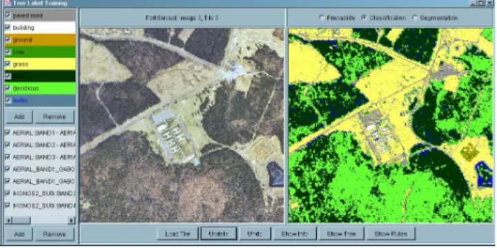
The GUI for label training is shown in Figure 5. The only interaction required is user’s providing of examples for land cover labels. These examples are input to the system using mouse clicks. The user can view the color composite image or individual data bands while entering examples in the training display. The GUI allows users to add both training and testing (ground truth) examples.
Each user can create a new model or update models previ-ously created by other users. At any time of the learning pro-cess, the user can validate the current classification model with the ground truth data using the automatically gen-erated confusion matrices. Advanced users can also change the parameters of the classification models through the GUI. The models can be stored either in the RDBMS or in a file.
4.2
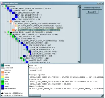
Tree and Rule Visualization
The GUI for tree visualization is shown in Figure 6. Each node in the tree shows the primary split condition and, for each label, percentages of training examples that satisfy that condition. Prediction importance of each data layer is mea-sured as the total reduction in the split criterion achieved by that data layer. Two Aerial bands, Gabor texture features and DEM were found to be the most important predictors in our experiments. Details of a node selected in the tree dis-play are also shown for further examination by an advanced user. These details include the number of training examples
Figure 5: GUI for label training. The panel on top-left shows the land cover labels defined by the user. The user can add new labels or remove existing ones, and can also change the color of a label. The panel on bottom-left shows the data layers used in train-ing. The user can add or remove layers using the corresponding buttons. Double-clicking on a data layer shows that layer in the left image panel. The “load tile” button loads a new image for training and/or classification. The “update” button shows the probability map for an individual label or the classification map for selected labels in the right im-age panel. The “show info” button displays informa-tion about the trained classifier. The “show tree” and “show rules” buttons open the tree and rule displays respectively.
Figure 6: GUI for tree visualization.
(size), the Gini or entropy impurity value (deviation), sur-rogate splits, path from the root node to the current node (original rule), and the generalized rule if it is a leaf node.
4.3
Tree and Rule Tracing
In tree tracing, the user can select a node in the tree and see which pixels/regions pass through that node during clas-sification. In rule tracing, the user can select a rule and see which pixels/regions are classified using that rule. Tracing also allows the user to select a pixel/region in the original image and see which node and rule are used to classify that pixel/region.
5.
PERFORMANCE EVALUATION
We evaluated the performance of the system using the four data layers (consisting of a total of 16 bands) described in Section 2. We present quantitative and qualitative results for pixel level and region level classification below.
5.1
Pixel Level Classification
5.1.1
Evaluation of classification with different data
layers
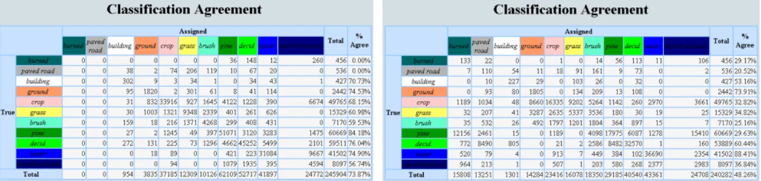
Examples of using different data layers for classification are given in Figure 7. The corresponding confusion matri-ces are given in Figures 8(a) and 8(b). Using all 16 bands resulted in a high classification accuracy of 72%. When we used only the bands with prediction importance higher than 2000 (7 bands), classification accuracy became slightly higher, because of better pruning and better classification of crop fields. Without the DEM band classification accura-cies for crop and brush dropped drastically. When we used only the visual bands (without the Gabor texture features and the DEM band), classification accuracy dropped close to 50%. Note that the confusion matrices show zero results for recognition of paved roads and burned areas. This is due to lack of qualified ground truth data as visual evaluation acknowledges correct classification of roads in many cases
(a) Using all 16 bands (b) Using 11 visual bands
Figure 7: Classification using all 16 bands from Aerial, Gabor, DEM, Ikonos versus using 11 visual bands from Aerial and Ikonos. We observe a good overall classification when all bands are used. With-out texture and DEM information more forest areas are misclassified as marsh or crop because the effects of shadows in noisy visual bands become more ap-parent in the absence of texture.
(see Section 5.2). Finally, we experimented with different parameter settings for the decision tree classifier. The dif-ferences caused by using different split functions were very subtle in our dataset.
5.1.2
Evaluation of rule generalization
The confusion matrix for classification using generalized rules is given in Figure 8(c). Classification accuracy for gen-eralized rules was very similar to (even slightly higher than) the one for the decision tree classifier. The improvement was due to the additional pruning during rule generalization.
5.1.3
Evaluation of classification with different
clas-sifiers
First, we compared decision tree classifiers with the mini-mum distance classifier (confusion matrix is given in Figure 8(d)). The minimum distance classifier cannot handle miss-ing data so we used only three Aerial and four Gabor bands for both classifiers. The decision tree classifier appeared superior, not only in its capability to handle numerical as well as categorical data and to cope with missing data val-ues, but also in regard to handling pure numerical feature data. The comparison showed an overall average classifica-tion accuracy of 48% using the minimum distance classifier compared to 64% using the decision tree classifier. Both experiments were performed using the same training and validation data for both classifiers.
We also compared decision tree classifiers with the un-supervised k-means clustering algorithm. We ran k-means using 11 clusters with three Aerial bands. Example classi-fications using the same three bands with the decision tree classifier, minimum distance classifier and k-means cluster-ing are given in Figure 9. As expected, unsupervised clus-tering resulted in the most noisy results. Some of the build-ing and grass pixels were classified correctly but most of the other labels were not separated successfully. Absence of Gabor features also caused the decision tree and minimum
(a) Using decision tree with all 16 bands from Aerial, Gabor, DEM and Ikonos
(b) Using decision tree with 7 bands (two Aerial, two Gabor, one DEM and two Ikonos) with prediction impor-tance over 2000
(c) Using rule-based classifier with 7 bands with predic-tion importance over 2000
(d) Using minimum distance classifier with three Aerial and four Gabor bands
Figure 8: Confusion matrices using different classifiers and data layers.
distance classifiers to produce noisy results but the decision tree classifier was the most successful in overall classifica-tion.
5.1.4
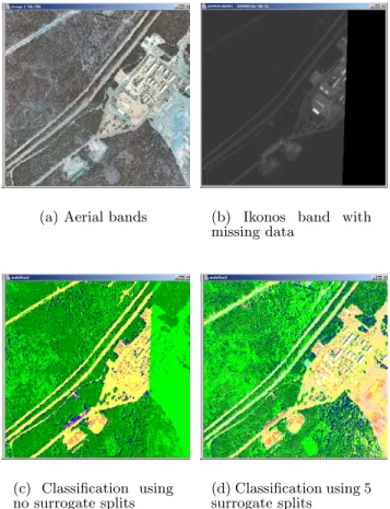
Evaluation of robustness to missing data
Figures 10 and 11 illustrate classification in the presence of missing data. Aerial and Ikonos bands were used in these examples. Missing data in the Ikonos bands initially re-sulted in many false alarms. However, land cover classifica-tion drastically improved when surrogate splits were used.5.2
Region Level Classification
The initial evaluation was done using a synthetic image that contained regions with circular, elliptical, square and rectangular shapes. Grouping these regions into different sub-classes showed that ECCENTRICITY is useful for dis-tinguishing compact shapes (square has a small value) from narrower and longer shapes (ellipse has a larger value and long rectangle has the largest value), THETA is useful for capturing rotation (vertical ellipse vs. rotated ellipse), IN-VARIANT 1 is useful for capturing circularity (square vs. circle), and SIGMA X is useful for capturing vertical vs. horizontal elongation (rectangles).
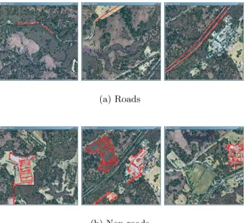
Another scenario where region features are useful is the learning of roads. It is very hard to distinguish paved roads from parking lots using pixel level classification because of
(a) Using decision tree classifier (b) Using minimum distance classifier (c) Using k-means cluster-ing
Figure 9: Classification using the decision tree sifier versus the supervised minimum distance clas-sifier and the unsupervised k-means clustering using the three Aerial bands and the same training data. Most of the labels were not separated successfully using unsupervised clustering. Absence of Gabor features also caused most of the noisy results.
(a) Aerial bands (b) Ikonos band with missing data (c) Classification using no surrogate splits (d) Classification using 5 surrogate splits
Figure 10: Classification in the presence of missing data. Missing data in the Ikonos bands (see Fig-ures 2(c) and 2(d)) causes the classification to give false results for the right half of the scene. However, recognition of buildings as well as land cover classi-fication drastically improves when surrogate splits are used.
their similar surface characteristics but roads have signifi-cantly different characteristics than parking lots in the re-gion level. We trained a decision tree classifier for the classes “roads” and “non-roads” using the segmented Fort data (some of the example regions are shown in Figure 12). The resulting rule was:
IF SIGMA_MINOR < 2.488 AND LABELID in {2}
THEN CLASS road WITH PROB 0.793701
This rule shows that SIGMA MINOR, i.e. the spatial vari-ance of a region along its minor axis, distinguishes very nar-row road regions from more rectangular parking lots. Note that the second condition in the rule requires that a road region consists of pixels classified as “paved” using the pixel level classifiers (see Table 1).
We also experimented with the statistical summaries of the pixel contents of regions in building region level land cover models. We computed the mean (ELEVATION MEAN) and standard deviation (ELEVATION STDDEV) of eleva-tion for each segmented region using the elevaeleva-tion attributes of pixels inside that region. These two values are included
(a) Aerial bands (b) Ikonos band with missing data and cloud
(c) Classification using no surrogate splits
(d) Classification using 5 surrogate splits
Figure 11: Classification in the presence of missing data (cont.). This scene has missing data at the bottom and left borders within the Ikonos bands as well as clouds within the Ikonos imagery. When no surrogate splits are used, land cover classification is rough and inaccurate, also the missing Ikonos layers cause misclassification in the lower bottom of the scene. When surrogate splits are used, strong cloud shadows still lead to slight misclassification of forest in the left half of the scene but overall accuracy is improved.
as new region level features in addition to the region shape features. We trained a decision tree classifier for the classes “flat fields” and “others” in a scenario of finding large and flat areas that are suitable for troop deployment. First, we chose large regions whose pixels were assigned to the “crop” or “grass” classes using the pixel level classifiers. Then, we input the regions that do not have hills in their neighbor-hood as examples for the “flat fields” class and the regions that were close to hills or lakes as examples for the “others” class. Some of the example regions and their corresponding elevation data are shown in Figure 13. The resulting rule was:
IF AREA >= 11452.5
AND ELEVATION_STDDEV < 2.51875 THEN CLASS flat field WITH PROB 0.820335
This rule shows that the decision tree classifier automat-ically captured the importance of area and uniformness of
(a) Roads
(b) Non-roads
Figure 12: Learning roads using region-based train-ing. Segmented region boundaries are marked with black. Example regions used in training are marked with red.
elevation (small standard deviation) from training examples. We believe that incorporating these region level rules with spatial relationships [2] (e.g. flat fields that are near a wide road that is connected to a village of interest) will provide remote sensing analysts with very valuable tools.
6.
CONCLUSIONS
We described decision tree and rule-based tools for build-ing statistical land cover models usbuild-ing our VisiMine system for interactive classification and mining of remote sensing image archives. The decision tree classifiers and the corre-sponding rules proved to be very powerful in building land cover models by fusing data from different numerical and categorical data layers. They were also very robust to miss-ing data and provided efficient land cover models with a small amount of training examples.
We compared the decision tree classifier with the rule-based classifier. Classification accuracy for generalized rules was very similar to (even slightly higher than) the one for the decision tree classifier. We also compared these two clas-sifiers with the unsupervised k-means clustering algorithm and the supervised minimum distance classifier. The deci-sion tree classifier appeared superior, not only in its capa-bility to handle numerical as well as categorical data and to cope with missing data values, but also in regard to handling pure numerical feature data. The Gabor features that we used as an additional ancillary data layer were also quite use-ful especially in smoothing noisy Aerial data. Micro-texture analysis algorithms like Gabor features are useful for mod-eling neighborhoods of pixels and distinguishing areas that may have similar spectral responses but have different spa-tial structures.
Our current work includes modeling interactions between multiple regions using region spatial relationships and using
(a) Flat fields: Aerial data
(b) Flat fields: DEM data
(c) Non-flat fields: Aerial data
(d) Non-flat fields: DEM data
Figure 13: Learning flat fields using region-based training. Examples regions used in training are marked with red.
teristic features that can distinguish different scene classes, and learning of decision forests as ensembles that use mul-tiple decision tree classifiers. We believe that incorporating spatial relationships information into the region level rules will help modeling of higher-level structures that cannot be modeled by individual pixels or regions and will provide re-mote sensing analysts with very valuable tools.
7.
ACKNOWLEDGMENTS
This work was done when Selim Aksoy was at Insight-ful Corporation and was supported by the U.S. Army con-tracts DACA42-03-C-16 and W9132V-04-C-0001. VisiMine project was also supported by NASA contracts NAS5-98053 and NAS5-01123.
8.
REFERENCES
[1] S. Aksoy, K. Koperski, C. Tusk, and G. M. J. C. Tilton. Learning Bayesian classifiers for a visual grammar. In Proceedings of IEEE GRSS Workshop on Advances in Techniques for Analysis of Remotely Sensed Data, pages 212–218, Washington, DC, October 2003.
[2] S. Aksoy, C. Tusk, K. Koperski, and G. Marchisio. Scene modeling and image mining with a visual grammar. In C. H. Chen, editor, Frontiers of Remote Sensing Information Processing, pages 35–62. World Scientific, 2003.
[3] L. Breiman, J. H. Friedman, R. A. Olshen, and C. J. Stone. Classification and Regression Trees. Wadsworth and Brooks/Cole, 1984.
[4] R. O. Duda, P. E. Hart, and D. G. Stork. Pattern Classification. John Wiley & Sons, Inc., 2000. [5] R. C. Gonzales and R. E. Woods. Digital Image
Processing. Addison-Wesley, 1993.
[6] G. M. Haley and B. S. Manjunath. Rotation-invariant texture classification using a complete space-frequency model. IEEE Transactions on Image Processing, 8(2):255–269, February 1999.
[7] R. M. Haralick and L. G. Shapiro. Computer and Robot Vision. Addison-Wesley, 1992.
[8] X. Huang and J. R. Jensen. A machine-learning approach to automated knowledge-base building for remote sensing image analysis with GIS data.
63(10):1185–1194, October 1997.
[9] K. Koperski, G. Marchisio, S. Aksoy, and C. Tusk. VisiMine: Interactive mining in image databases. In Proceedings of IEEE International Geoscience and Remote Sensing Symposium, volume 3, pages 1810–1812, Toronto, Canada, June 2002.
[10] P. Langley and H. A. Simon. Applications of machine learning and rule induction. Communications of the ACM, 38:55–64, November 1995.
[11] R. L. Lawrence and A. Wright. Rule-based classification systems using classification and regression tree (CART) analysis. Photogrammetric Engineering & Remote Sensing, 67(10):1137–1142, October 2001.
[12] R. J. A. Little and D. B. Rubin. Statistical Analysis with Missing Data. John Wiley & Sons, Inc., 1987. [13] B. S. Manjunath and W. Y. Ma. Texture features for
browsing and retrieval of image data. IEEE Transactions on Pattern Analysis and Machine Intelligence, 18(8):837–842, August 1996.
[14] M. Musavi, P. Natarajan, S. Binello, and J. McNeely. Knowledge based extraction of ridge lines from digital terrain elevation data. In Proceedings of IEEE International Geoscience and Remote Sensing Symposium, volume 5, pages 2492–2494, 1999. [15] NASA. TERRA: The EOS flagship.
http://terra.nasa.gov.
[16] J. R. Quinlan. C4.5: Programs for Machine Learning. Morgan Kaufmann Publishers, 1993.
[17] J. Rogan, J. Miller, D. Stow, J. Franklin, L. Levien, and C. Fischer. Land-cover change monitoring with classification trees using Landsat TM and ancillary data. Photogrammetric Engineering & Remote Sensing, 69(7):793–804, July 2003.
[18] L.-K. Soh and C. Tsatsoulis. Multisource data and knowledge fusion for intelligent SAR sea ice classification. In Proceedings of IEEE International Geoscience and Remote Sensing Symposium, volume 1, pages 68–70, 1999.
[19] T. M. Therneau and E. J. Atkinson. An introduction to recursive partitioning using the RPART routines. Technical Report 61, Department of Health Science Research, Mayo Clinic, Rochester, Minnesota, 1999.