A Kuznets Curve in Environmental Efficiency:
An Application on OECD Countries
OSMAN ZAIM and FATMA TASKIN
Department of Economics, Bilkent University, 06533, Bilkent, Ankara, Turkey (e-mail: [email protected])
Accepted 9 June 1999
Abstract. The role of the environment is an important issue in policy making and the accurate
assessment of the environmental conditions is vital. In this paper, using nonparametric techniques, an environmental efficiency index is developed for each of the OECD countries. These indexes allow one both to do cross section comparisons on the state of each country’s production process in its treatment of undesirable outputs and also to trace each country’s modification of their production processes overtime. Furthermore in this study we investigate the factors underlying societies’ environmental concerns that eventually lead to changes in the environmental efficiency. The results provide further empirical evidence for the environmental Kuznets curve hypothesis.
Key words: environmental efficiency index, environmental Kuznets curve, nonparametric efficiency
measurement
JEL classification: P24, O12, Q25
1. Introduction
The relation between economic growth and environmental degradation has been the focus of many recent studies. The increased awareness on environmental issues have initiated many studies to analyze the relation between economic growth and environmental degradation. In their pioneering study, Grossman and Krueger (1993) established the empirical relationship between measures of environmental quality and national income while examining the likely environmental impacts of the North American Free Trade Agreement. An inverted U-type relationship, commonly referred as the environmental Kuznets curve, has been established between the levels of emissions and income, implying that environmental degra-dation increases with income at low levels of income and then decreases once a threshold level of per capita income level is reached (Grossman and Krueger 1995). Studies such as Shafik and Bandyopadhyay (1992), Cropper and Griffith (1994), Selden and Song (1994) and Holtz-Eakin and Selden (1995) investigated this relationship for alternative measures of environmental degradation measured either with levels of pollutants or pollutant intensities.1 These studies presented the inverted U-curve relationship as an observation of an ‘empirical phenomena’
without investigating the underlying mechanism that generates growth and emis-sions of pollutants. The only explanation provided is that once a country reaches a certain standard of living then the concern about environment will become relevant and necessary institutional, legal and technological adjustments will be made to decrease the environmental degradation.2
Moreover, these studies disregarded the fact that the two variables (per capita GNP and levels of emissions or per capita emissions) in the Kuznets curve analysis are the outcomes of a production process and that this reduced form approach fails to recognize the underlying production process which converts the inputs into outputs and pollutants. In fact, it is the modification or transformation of this production process that may lead to the improvement in the environmental efficiency at higher income levels.
Studies that given emphasis to the transformation of the production process and aim at quantifying the opportunity cost of adopting an environmentally more desirable production process are the ones which employ production frontier tech-niques. For example Fare et al. (1986, 1989b), Fare et al. (1989a) and Fare et al. (1994b) concentrated on the analysis of micro-level data to develop an environ-mental performance indicator. The starting point of these studies is the recognition that pollutants are not freely disposable, that is, some productive resources have to be given up in order to reduce the level of pollutants. This requires transformation of the production process from one where all outputs (good or bad) are strongly disposable (with no cost) to the one which is characterized by weak disposability where the disposability of bad output(s) is limited (through making the disposal of bads costly). Then, one can claim that it is the extent of the required output sacrifice due to this transformation which determines environmental efficiency and its improvement in a society.
As environmental concerns are increasingly pronounced in relation to global commons, countries are forced to undertake such institutional reforms that would compel private users of environmental resources (and producers of environmental bads) to take into account the social cost of their actions which ultimately leads to the aforementioned transformation of the production processes. Recognizing the importance of measuring the cost of such transformation at the country level, the objective of this study is two-fold. The first is to develop an environmental efficiency index for each of the OECD countries that would allow one to do both cross-section and overtime comparisons on the state of each country’s produc-tion process in its treatment of undesirable outputs. The second objective is to examine the existence of a Kuznets type relationship for environmental efficiency as measured by this index.
The paper is organized as follows. Section 2 provides the model that will be used for the computation of an environmental efficiency index. Section 3 is allocated to the presentation of the data source and discussion of results. Finally, Section 4 concludes.
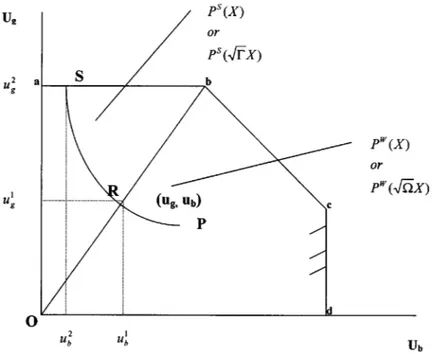
Figure 1. Output sets for strongly and weakly disposable undesirable outputs.
2. Model
In the theory of production, it is common to assume that outputs are strongly disposable, which implies that the disposal of any output can be achieved without incurring any cost in terms of reduced production of other outputs. However, the symmetric treatment of outputs in terms of their disposability characteristics looses its justification if one or some of the outputs produced are undesirable goods such as carbon dioxide production (as a by-product) along with the cement production. Especially in regulated environments, where producing units are forced to clean up the undesirable outputs that they produce or forced to reduce their levels of undesirable output production, one has to treat undesirable and desirable outputs asymmetrically in terms of their disposability characteristics. Even in the absence of regulations, increased environmental consciousness in the society3still requires the treatment of undesirable goods as weakly disposable, i.e. their disposal is achieved by reducing the desirable outputs proportionately.
The environmental efficiency indexes are developed by comparing the produc-tion processes under alternative assumpproduc-tions on disposability. One such environ-mental efficiency index developed by Fare et al. (1989a) adopts an hyperbolic graph efficiency approach. To explain the underpinnings of the method one can use Figure 1 which represents the output sets for two (piecewise linear) technologies with different assumptions on disposability of bads.
In Figure 1, where Ugand Ubdenote desirable output (“good”) and undesirable output (“bad”) respectively, if the disposal of bad is costless, the line segment ab
would be a feasible part of the technology since a reduction in Ub (a movement from b towards a) would be possible without giving up any Ug. If however the disposal of Ubis not costless the line segment ab will not be a feasible part of the technology. This is because some resources would be pulled out of the production of Ugin order to clean up Ubwhich in turn would imply production of Oa amount of Ug is no longer feasible. Then we say that the technology bounded by line segments Oa, ab, bc and cd represents the strongly disposable output technology
PS(x), and the technology bounded by line segments Ob, bc and cd represents technology with weakly disposable bads4PWb(x).
To describe the theoretical background of the model used, suppose we observe a sample of K production units, each of which uses inputs x ∈ RN+ to produce desirable outputs y∈ RM+, and undesirable outputs w∈ RJ+. As a matter of notation, let xki be the quantity of input i used by unit k and let yki and wki be the quantity of desirable and undesirable output i produced by unit k respectively. These data can be placed into data matrixes M, a K × M matrix of desirable output levels whose k,i’th element is yki, J, a K × J matrix of undesirable output levels whose
k,i’th element is wki and N a K× N matrix of input levels whose k,i’th element is
xk
i. Using the notation at hand and assuming that the production process satisfies strong disposability of both outputs (good and bad) and inputs, the constant returns to scale (CRS) output set5PS(x) (bounded by Oa, ab, bc and cd in Figure 1) can be constructed from observed data by means of
PS(x)= {(y, w) : zTM≥ y, zTJ≥ w, zTN≤ x, z ∈ R+K}
where z is a K× 1 intensity vector. Similarly, a CRS technology satisfying the weak disposability of undesirable outputs and strong disposability of desirable outputs and inputs can be represented as an output set as shown below:
PW(x)= {(y, w) : zTM≥ y, zTJ= w, zTN≤ x, z ∈ R+K}
Intuitively, these equations6 construct a reference technology from the observed inputs and outputs relative to which technical efficiency of each producing unit can be calculated. The next step in the construction of the environmental efficiency index is the computation of the opportunity cost of transforming the production process from one where all outputs are strongly disposable to the one which is characterized by weak disposability of undesirable outputs. Fare et al. (1989a) define this opportunity cost as the ratio of two hyperbolic graph measure of tech-nical efficiencies measured with respect to two technologies characterized by two different disposability assumptions. The hyperbolic graph measure of technical efficiency seeks the maximum simultaneous equiproportionate expansion for the desirable outputs and contraction for the inputs and undesirable outputs.
For a CRS technology which satisfies strong disposability of inputs and outputs (good or bad) hyperbolic graph measure of technical efficiency measure is defined as:
and for each producing unit k0it can be computed as the solution to the following programming problem: FgS(xk0, yk0, wk0)= minλ (LP1) subject to zTM≥ λ−1yk0 zTJ ≥ λwk0 zTN ≤ λxk0 zT ∈ RK+ or equivalently FgS(x k0 , yk0, wk0)= min0 (LP2) subject to ZTM ≥ yk0 ZTJ ≥ 0wk0 ZTN ≤ 0xk0 ZT ∈ R+K
For computational purposes the nonlinear programming problems (in LP1) are converted into linear programming problems (as in LP2), where 0 = λ2 and Z =
λz and the solution is derived by solving for √0. Note here that for any (xk0, yk0,
wk0)∈ GR, FS g(xk
0
, yk0, wk0)∈ (0,1] and measures the maximum equiproportionate deflation of all inputs and undesirable outputs and inflation of all outputs that remain technically feasible.
For a technology that assumes weak disposability for the undesirable outputs and strong disposability for the desirable outputs and inputs, a linear programming problem FgW(xk0, yk0, wk0)= min (LP3) subject to ZTM ≥ yk0 ZTJ = wk0 ZTN ≤ xk0 ZT ∈ R+K
can be constructed to obtain a graph measure of technical efficiency for each producing unit k0 as the solution to√. If one translates these measures into a
figure, in Figure 1, while computing the hyperbolic graph measure of technical efficiency of a production plan denoted by (ug, ub) at point P with respect to a technology which assumes strong disposability of outputs, point P is compared to point S where the good output is expanded (u2
g = ug/ √
0) while simultaneously
contracting inputs and the bad output (u2b = √0ub) in the relevant output set (PS(√0x)).7 Similarly, the hyperbolic graph measure of technical efficiency of production plan (ug, ub), with respect to a technology which assumes weak dispos-ability of undesirable good, compares point P to point R where the good output is expanded (u1g = ug/
√
) while simultaneously contracting inputs and the bad
output (u1b=√ub) in the relevant output set (PW( √
x)).8
Finally, the environmental efficiency index which shows potential desirable output loss which stems from reduced disposability of undesirable output can be obtained from the ratio of these two efficiency scores as
H =
√
0
√
.
This measure takes a value 1 only for those producing units which are on the segments bc and cd or for those producing units whose hyperbolic expansions fall on these segments. Note that the efficiency index for production plans located on these line segments correctly signals high efficiency in the sense that these units cannot reduce the bad output while simultaneously expanding the good output and contracting the inputs.9 Furthermore, due to the fact that line segments bc and cd are common to both technologies with different assumptions on the disposability of bads, for those producing units it is only natural to expect no opportunity cost of transforming the production process from one where all outputs are strongly disposable to the one which is characterized by weak disposability of undesirable outputs. Hence being environmentally efficient implies choosing the appropriate production plan (i.e. a mix of desirable output, undesirable output and inputs) which will not be constrained by the effective regulation that prohibits the free disposal of undesirable goods. For producing units which are located along the line segment Ob, or in the interior part of the weakly disposable output set whose hyper-bolic expansions falls on the line segments Ob and ab, the H index will assume values less than 1, indicating that there is an opportunity cost due to aforemen-tioned transformation. This opportunity cost, expressed in terms of the percentage desirable output to be given up due to the reduced disposability of undesirable output, or in terms of additional input required to clean up the undesirable output to comply with the effective regulations, can be measured as 1− H. Therefore H can safety be used as a measure of environmental efficiency.
Note however that this measure of environmental efficiency differs from more crude measures of environmental performance such as pollution per output. To better comprehend the difference between these two measures of environmental performance, one should note that for all production plans whose hyperbolic expan-sions fall on the line segments Ob and ab, H measures the respective relative
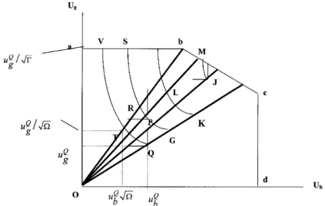
Figure 2. Hyperbolic graph measure of technical efficiencies and environmental efficiency
magnitudes of the hyperbolic distances between Ob and ab and assigns rela-tively higher values to those producing units whose hyperbolic expansion to the line segment Ob corresponds to larger desirable output. The relationship between pollution per output and the H index is also illustrated in Figure 2 in which the environmental efficiency of the two producing units (Q and P) with different pollu-tion per output ratios are compared with the H index. Although producing units Q and P have different pollution per output ratios, while comparing the environmental efficiency of these two units through H, we first account for this difference by scaling the respective desirable and undesirable outputs (and also inputs) by the hyperbolic expansion factors so as to bring them to the lowest permissible undesir-able output to desirundesir-able output ratio (i.e. uQg/QuQb at T is equal to uPg/puPb at R) defined by the Ob boundary of the weakly disposable output set and then we compare the magnitude of the hyperbolic distances VT and SR, i.e.,
HQ= uQ g/ p Q uQg/ p 0Q = s 0Q Q and HP = uP g/ √ P uP g/ √ 0P = s 0P P .
As it is obvious from the figure, producing unit P with the lower bad over good ratio will be deemed more environmentally efficient than producing unit Q since it produces more of the desirable good after accounting for the differences in bad over good ratios. Furthermore, one can also generalize this result by noting that of the two units with the same bad over good ratio (i.e. Q and K in Figure 2), the one which produces larger amount of desirable output will be measured as being more environmentally efficient. Figure 2 also highlights how a producing unit can increase its environmental efficiency from one period to another. A producing unit
can increase its environmental efficiency either by expanding their desirable output by maintaining the same pollution per output ratio (i.e. by moving from point Q to K) or by expanding their desirable output at a higher rate than the undesirable output (i.e. by moving from Q to P or L) and hence lowering its pollution per output ratio. If the changes in environmental efficiency overtime is positively related to pollution per output ratio, this is an indication that producing units are not only choosing production plans that are less (more) vulnerable to a departure from strong disposability of undesirable outputs but also the ones with lower (higher) pollution per output ratios among the alternatives which would bring about the same change in H (that is a move from Q to P rather than Q to G).
3. Data and discussion of results
While computing the environmental efficiency indexes for each of the OECD countries,10 we chose aggregate output measured by real Gross Domestic Product (GDP) expressed in international prices (in 1985 U.S. dollars) as the desirable output and carbon dioxide (CO2) emissions (millions of tons) as the only undesir-able output. The two inputs considered are aggregate labor input measured by the total employment and total capital stock. The input and the desirable output data are compiled from the Penn World Tables (PWT 5.6) initially derived from the Interna-tional Comparison Program benchmark studies where cross-country and overtime comparisons are possible in real values. Pollution-related data are obtained from Environmental Data Compendium 1995.
In developing the environmental efficiency index, we used cross-section data on all countries to solve the linear programming problems (LP2) and (LP3) for each country. The solutions determine the efficiency of each country, for a given year, with respect to two OECD multi-output production frontiers constructed under two alternative disposability assumptions for the undesirable output. The ratio of these two efficiency measures renders a particular country’s index of environmental efficiency for a given year. This computation is repeated for each year between 1980 until 1990 to analyze the development of environmental efficiency indexes overtime. The resulting efficiency indexes are presented in the Appendix.
To illustrate the computation of each environmental efficiency index and to interpret the relative differences in environmental efficiency, Table I presents the results for four selected countries for the year 1987. In this table, U.S.A., which is perfectly efficient as measured by the hyperbolic graph measure of technical efficiencies with respect to the two technologies characterized by strong and weak disposability of bads, is environmentally efficient with an H value equal to one. This indicates that a regulation which restricts the free disposability of carbon dioxide will not be binding for U.S.A. Another country such as Ireland, with the same hyperbolic graph measure of technical efficiency values with respect to both technologies, is of equal hyperbolic distance from the boundaries of both output sets and will again by unaffected by a similar regulation.
Table I. Hyperbolic graph measure of technical efficiency and environmental
efficiency values for selected countries.
Country Points on √0 √ H index Carbon dioxide
Figure 2 per GDP (tons
per $1000 GDP)
USA M 1.000 1.000 1.000 1.13
Ireland J 0.845 0.845 1.000 1.16
Sweden T 0.887 1.000 0.887 0.48
Germany K 0.898 0.904 0.993 1.29
On the other hand Sweden, who is technically efficient with respect to weakly disposable bad technology but inefficient with respect to strongly disposable tech-nology, is located along the line segment Ob (exclusive of point b) and has an environmental efficiency index less than one, indicating an opportunity cost of a binding regulation which is equal to 11.3% (i.e. 1–0.887) of its GDP. Finally, a country such as Germany, having hyperbolic graph measure of technical efficiency scores less than one, is an interior element of the weakly disposable output set bounded by the line segments Ob, bc and cd and its hyperbolic expansions falls on
ab and Ob segments. Combining this information with the observed carbon dioxide
per GDP ratios, the relative position of each country can approximately be shown with points M, J, T and K for USA, Ireland, Sweden and Germany respectively.
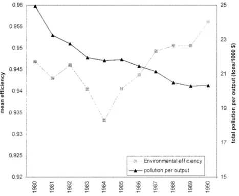
Leaving the disaggregated results on the environmental efficiency of each country through time to the Appendix, in Figure 3 we plot the mean value of the environmental efficiency index computed over the 25 countries for the period 1980–1990. The mean index shows the lowest environmental efficiency in terms of carbon dioxide emissions in 1984 and an improved environmental performance since then. We observe that, for the period 1980–1990, there has been a positive association between the changes in the environmental efficiency index H and vari-ations in carbon dioxide emissions per GDP, an environmental quality measure which previous studies on environmental Kuznets curve tried to explain. In the figure, declining environmental efficiency between the years 1982 and 1984 is simultaneously observed with dampened general decline in carbon dioxide emis-sion per output. Similarly, from 1985 to 1988, the rapid decline in total carbon dioxide emission per output occurred concurrently with improved environmental efficiency. This is an indication that, over time, the OECD countries have been choosing production plans that are not only less vulnerable to a departure from strong disposability of undesirable goods but also the ones with lower pollution per GDP ratios.
The analysis of individual country experiences reveals that among 25 countries, U.S.A., Luxembourg, U.K., Iceland are among the best five performers and Japan, Turkey, Sweden, New Zealand and France are among the worst five, on the basis
Figure 3. Relation between environmental efficiency and environmental quality in the OECD.
of mean environmental efficiency computed over 1980–1990. Despite the differ-ences in overall means countries such as Mexico, Portugal, and Turkey showed improved performance while countries like Sweden, Austria and France exhibited a deteriorating environmental performance over time.
One other issue of concern is to determine the factors underlying the changes in the environmental efficiency. We expect that specific attributes of an individual country contribute to the social and economic climate regarding environmental issues. The attributes that we expect will influence environmental efficiency are the ones considered in a typical Kuznets curve analysis. For this purpose, in a panel data framework, we examined the relationship between the environmental efficiency index and the variables such as GDP per capita, population density, environmental public research and development expenditures per GDP and share of manufacturing value added in GDP. The source for the last two variables is the OECD Environmental Compendium 1995 and the manufacturing shares are computed from the National Accounts (1991).
Letting Hit represent the environmental efficiency of country i in year t, the equation below specifies a possible form relation between the environmental efficiency and the variables discussed above.
Hit = β1i+ β2GDPPCit + β3(GDPPC)2it + β4(GDPPC)3it+ β5POPDENSit +β6RESEXPit + β7MANSHAREit + β8(MANSHARE)2it+ εit
where: i is country index; t is time index; ε is the disturbance term with mean zero and finite variance; GDPPC is GDP per capita; POPDENS is population density; RESEXP is environmental research and development expenditures11 and MANSHARE is share of manufacturing in GDP.
The shape of he polynomial will expose the relationship between environmental efficiency and GDP per capita. A positive sign for GDPPC coupled with a negative sign for its quadratic and a positive sign for its cubic terms will imply an improving environmental performance at the initial phases of growth which is followed by a phase of deterioration and then a further improvement once a critical level of per capita GDP is reached. A positive sign is expected for population density vari-able since in more densely populated areas there will be more pressure for the improved environmental efficiency.12 A positive association is expected between environmental efficiency and environmental research expenditures. For the manu-facturing share variable, we expect a quadratic relationship between environmental efficiency and GDP per capita variable implying a deterioration in environmental efficiency at the initial phases of industrialization and then an improvement once a critical level of industrialization is reached.
There are alternative specifications of the cross-section time-series models which mainly differ in their treatment of the intercept of the equation. If the β1i are assumed to be fixed parameters, then the model is known as fixed effects model. If on the other hand β1iare assumed to be random variables that are expressed as β1i= ¯β1+ µi, where ¯β1is an unknown parameter and µi are independent and identically distributed random variables with mean zero and constant variance, then the model is called random effects model. The disadvantage of the fixed effects model is that there are too many parameters to be estimated and hence loss of degrees of freedom which can be avoided if we either assume the same intercept for all the cross-sectional units or assume β1ito be random variables. Nevertheless, random effects model is not totally free from problems. In cases where µi and other independent variables are correlated, the random effects model is similar to an omitted variable specification which will lead to biased parameter estimates, making a fixed effects model a more appropriate choice. In examining the relationship between environ-mental indexes and economic and social factors, relevant tests will be performed to determine the most suitable estimation form.
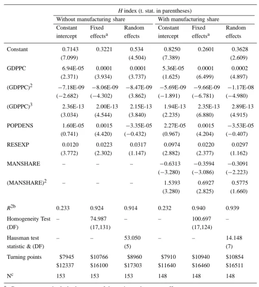
Table II provides the parameter estimates of the regressions for the H index under alternative specifications. The possibility of a causal relationship between gross domestic product per capita and manufacturing share in gross domestic product limits the use of manufacturing share as an explanatory variable in all specifications. The first three columns of the table report the estimation results when the manufacturing share in GDP is excluded from the models and the last three columns are the parameter estimates of models where the manufacturing share is included as an independent variable. In each case, columns one and two provide the parameter estimates of the fixed effects model with a common intercept
Table II. Parameter estimates for alternative models.
H index (t. stat. in parentheses)
Without manufacturing share With manufacturing share
Constant Fixed Random Constant Fixed Random
intercept effectsa effects intercept effectsa effects
Constant 0.7143 0.3221 0.534 0.8250 0.2601 0.3628
(7.099) (4.504) (7.389) (2.609)
GDPPC 6.94E-05 0.0001 0.0001 5.36E-05 0.0001 0.0002
(2.371) (3.934) (3.737) (1.625) (6.499) (4.897) (GDPPC)2 −7.18E-09 −8.06E-09 −8.47E-09 −5.69E-09 −9.66E-09 −1.17E-08
(−2.682) (−4.302) (3.862) (−1.891) (−6.781) (−4.980) (GDPPC)3 2.36E-13 2.00E-13 2.15E-13 1.94E-13 2.35E-13 2.89E-13
(3.034) (4.544) (3.840) (2.235) (6.880) (4.915)
POPDENS 1.60E-05 0.0015 −3.35E-05 2.27E-05 0.0015 −3.53E-05
(0.741) (4.420) (−0.432) (0.967) (4.204) (−0.407) RESEXP 0.0120 0.0223 0.0317 0.0974 0.0220 0.0297 (3.772) (2.302) (1.147) (2.882) (2.377) (1.162) MANSHARE – – – −0.6313 −0.3594 −0.3091 (−3.280) (−3.086) (−2.223) (MANSHARE)2 – – – 1.5393 0.6927 0.5775 (3.280) (2.825) (1.660) R2b 0.233 0.924 0.914 0.232 0.940 0.939 Homogeneity Test – 74.987 – – 100.697 – (DF) (17,131) (17,124) Hausman test – – 53.050 – – 14.148 statistic & (DF) (5) (7) Turning points $7945 $10766 $8960 $7910 $10940 $10854 $12337 $16100 $17303 $11640 $16460 $16511 Nc 153 153 153 148 148 148
a Constant terms include the mean of the estimated country effects. b R2of the unweighted regression is reported.
c 17 countries are included into the regression due to the availability of the variables.
and fixed effects model with country specific intercepts respectively. The third columns are reserved for the parameter estimates of the random effects model.
In both cases, an F test performed on the alternative specifications of the fixed effects model rejects the null hypothesis of a common intercept in favor of the model with country specific intercept terms. Furthermore, the choice between the fixed effects model and the random effects model can be made using the Hausman test. The Hausman test has an asymptotic χ2
k−1 distribution and in both cases we reject the null hypothesis which suggests that the random effects model is the appropriate specification.
The most apparent outcome in all the specifications of the model is that the vari-ables GDP per capita, its quadratic and cubic terms are statistically significant and their respective signs imply an improving environmental performance at the initial phases of growth (up to an income level of approximately $11 000 according to the fixed effects model) which is followed by a phase of deterioration and then a further improvement once a critical level of per capita GDP (approximately $16 000) is reached. This is actually another representation of the environmental Kuznets curve relationship which mainly holds for countries at income levels of $11 000 and over. For these countries the initial deterioration of environmental conditions and its improvement in latter stages of economic growth manifest itself as an initial decline and then an improvement of environmental efficiency as measured by our indexes. This is an indication that the opportunity cost of the transformation of a production process from one where undesirable outputs are strongly disposable towards the one that they are weakly disposable become smaller after a certain threshold income level. Note that the estimate of this critical level of income of approximately $16 000 at which environmental efficiency begins to improve is robust with respect to alternative specifications of the fixed effects model.
The estimated relationship between H and GDP per capita predicts improving environmental efficiency with increasing income, at income levels below approxi-mately $11 000 per capita GDP. This explains the improvement in the environ-mental efficiency index H which is simultaneously observed with income increases in countries like Mexico, Greece, Ireland, Portugal and Turkey.13
The positive and consistently significant coefficient estimate for the popula-tion density and research and development expenditures per GDP variables in fixed effects models are an indication that densely populated countries among the OECD group are more likely to be concerned about increasing environmental efficiency and that expenditures to improve environmental conditions have in fact a considerable positive impact on environmental efficiency.
Another variable we have considered that would affect the environmental effi-ciency is the share of manufacturing value added in the GDP. The examination of the second part of Table II reveals that, in addition to the relationship between GDP per capita and environmental efficiency, the share of manufacturing value added in GDP variable exhibits a U-curve type quadratic relationship with the environmental efficiency. This is an indication that there is a threshold level of industrialization above which environmental efficiency increases.
In summary, the results indicate that for environmental efficiency, which is one important component of the environmental quality, we observe an environmental Kuznets type relationship with respect to per capita GDP, after accounting for such factors as population density and environmental research expenditures. This shows that the opportunity cost of adopting environmentally more desirable production processes, which prohibits the free disposal of carbon dioxide, decreases after a certain threshold level of per capita income.
5. Conclusion
This paper, using production frontier analysis, develops an environmental effi-ciency index for the purpose of cross country and overtime comparisons. The particular emphasis is on the transformation of the technology to provide an insight to the environmental Kuznets curve relationship commonly referred as inverted U-curve hypothesis. The study develops an alternative index which aims at measuring the opportunity cost of adopting an environmentally desirable technol-ogies for OECD countries. As opposed to methods which gauge the environmental quality with the levels of emissions of pollutants, the index that is derived in this study is based on a production approach that differentiates between the disposa-bility characteristics of the environmentally desirable and undesirable outputs. The closer inspection of the index reveals that there is a deterioration in environmental efficiency starting at income levels of $11 000 and an improved environmental performance once the critical level of income ($16 000) is reached. This finding is similar in spirit to the results obtained in a typical environmental Kuznets curve analysis but goes one step further in measuring the opportunity cost of the transformation of the production process.
Notes
1. Total and annual deforestation in Shafik and Bandyopadhyay (1992), rate of deforestation in Cropper and Griffith (1994), various air pollutants per capita in Selden and Song (1994) and Carbon dioxide per capita in Holtz-Eakin and Selden (1995) are all related to per capita income and some other control variables.
2. Further evidence on the issue is provided by Xepapadeas and Amri (1998), who found a positive association between the probability of having acceptable environmental quality and state of economic development in a univariate and ordered probit models framework.
3. This may ultimately lead them to willingly incur some costs to reduce the levels of the undesirable products.
4. Note here that we refrain from using the terminology ‘weakly disposable output technology’ since we still maintain strong disposability assumption on environmentally non-hazardous goods. The weakly disposable output technology would be bounded by Ob, bc, cO (not drawn on the figure).
5. The output set denotes the collection of all output vectors y∈ RM+ and w∈ RJ+that are obtainable from the input vector x∈ RN+.
6. Equivalently one may chose to define the reference set for a strongly disposable technology and for a weakly disposable technology using a graph measure as
GRS = {(x, y, w) : zTM≥ y, zTJ≥ w, zTN≤ x, z ∈ R+K} and GRW = {(x, y, w) : zTM≥ y, zTJ= w, zTN≤ x, z ∈ RK+}
respectively. The graph of the technology is the collection of all feasible input and output vectors (for definition see Fare et al. (1994a)).
7. The expression (PS(√0x)) denotes the strongly disposable output set (Oa, ab, bc and cd) after contracting the inputs by the scalar√0, which is positive but less than or equal to one. 8. The expression (PW(√x)) denotes the weakly disposable output set (Ob, bc and cd) after
9. Note for example along the line segment bc a producing unit can not contract its undesirable output and expand its desirable output along a hyperbolic path and still remain in the relevant output sets PS(√0x) and PW(√x). More formally, it is said that points along the line bc are the elements of the efficient subset of graph which finds its expression as:
Eff GR := {(x, ug, ub): (x, ug, ub)∈ GR, (x0,−u0g, u0b)≤ (x, −ug, ub)⇒ (x0,−u0g, u0b) /∈ GR}.
For a more comprehensive discussion on the graph and its subsets see Fare et al. (1985). 10. The OECD countries are: Canada, Mexico, USA, Japan, Austria, Belgium, Denmark, Finland,
France, Germany, Greece, Iceland, Ireland, Italy, Luxembourg, Netherlands, Norway, Portugal, Spain, Switzerland, Turkey, UK, Australia and New Zealand.
11. These are the public research and development financing for environmental protection in terms of per $1000 of GDP at 1985 prices and PPPs.
12. For the effect of the population density variable on environmental performance, there are alterna-tive prior expectations in the literature. For example, in Selden and Song (1994) it is hypothesized that ‘sparsely populated countries are likely to be less concerned about reducing per capita emis-sions, at every level of income, than more densely populated countries’. In Cropper and Griffiths (1994), on the other hand, high population density is found to be a major cause of increased deforestation, indicating a negative relationship between population density and environmental performance.
13. These are the countries with per capita income below $11 000 in our sample.
Appendix Table AI. H index.
1980 1981 1982 1983 1984 1985 1986 1987 1988 1989 1990 Mean Canada 0.98355 0.98197 0.98849 0.98227 0.98015 0.97829 0.97847 0.97912 0.98041 0.98380 0.97595 0.98113 Mexico 0.90631 0.92572 0.89378 0.87939 0.90532 0.93664 0.93820 0.97895 0.98670 0.99137 1.00000 0.94022 USA 1.00000 1.00000 1.00000 1.00000 1.00000 1.00000 1.00000 1.00000 1.00000 1.00000 1.00000 1.00000 Japan 0.88697 0.89657 0.87417 0.86343 0.86443 0.83460 0.83003 0.83754 0.86082 0.86742 0.89603 0.86473 Austria 0.94061 0.92221 0.92845 0.91586 0.90057 0.90181 0.90474 0.90365 0.90191 0.90269 0.91437 0.91244 Belgium 0.97459 0.96806 0.97497 0.96083 0.94850 0.94930 0.95120 0.94890 0.94793 0.94772 0.95178 0.95671 Denmark 0.94317 0.92640 0.94383 0.92937 0.91793 0.93558 0.93964 0.93400 0.92918 0.92161 0.93544 0.93238 Finland 0.95694 0.93732 0.94983 0.93611 0.91878 0.93793 0.94234 0.95090 0.93806 0.93791 0.93370 0.93998 France 0.93645 0.92361 0.93709 0.92353 0.90277 0.90083 0.89721 0.89481 0.89850 0.90035 0.90789 0.91119 Germany 0.99647 0.99588 0.99737 0.99635 0.99390 0.99433 0.99567 0.99286 0.98941 0.98343 0.97090 0.99151 Greece 0.90850 0.91721 0.90966 0.92215 0.92056 0.94421 0.93599 0.96351 0.96986 0.97387 0.97663 0.94019 Iceland 1.00000 1.00000 1.00000 1.00000 1.00000 1.00000 1.00000 1.00000 0.98678 0.96484 1.00000 0.99560 Ireland 0.98870 0.98582 0.98535 0.98321 0.97867 0.98600 1.00000 1.00000 0.99734 1.00000 1.00000 0.99137 Italy 0.94120 0.92647 0.93959 0.92823 0.91175 0.91582 0.92253 0.92614 0.93296 0.93452 0.94479 0.92945 Luxembourg 1.00000 1.00000 1.00000 1.00000 1.00000 1.00000 1.00000 1.00000 1.00000 1.00000 1.00000 1.00000 Netherlands 0.96150 0.95730 0.95556 0.95002 0.94232 0.94735 0.95649 0.95627 0.95966 0.95927 0.96731 0.95573 Norway 0.94384 0.93339 0.94120 0.93111 0.91394 0.92249 0.92890 0.92167 0.91301 0.91814 0.91263 0.92548 Portugal 0.90609 0.88924 0.88791 0.89190 0.88089 0.90595 0.92940 0.94613 0.98185 1.00000 1.00000 0.92903 Spain 0.94033 0.94814 0.94606 0.94253 0.91855 0.91491 0.91718 0.92589 0.93070 0.93774 0.93474 0.93244 Sweden 0.92690 0.91697 0.92329 0.90595 0.88560 0.88574 0.88964 0.88718 0.89384 0.87664 0.87500 0.89698 Switzerland 0.96549 0.96069 0.97055 0.95891 0.93510 0.93996 0.94341 0.94051 0.93671 0.93580 0.93042 0.94705 Turkey 0.81173 0.80454 0.81085 0.83506 0.85571 0.91222 0.92212 0.97138 0.95404 0.94320 0.97361 0.89041 UK 0.99629 0.99412 0.99722 0.99800 0.99782 1.00000 1.00000 1.00000 1.00000 1.00000 1.00000 0.99850 Australia 0.97325 0.97222 0.98549 0.97640 0.97021 0.97015 0.97023 0.97087 0.96672 0.97205 0.97644 0.97309 N. Zealand 0.88120 0.89173 0.91064 0.90087 0.88880 0.90168 0.89863 0.90101 0.90686 0.91329 0.92696 0.90197 Mean 0.94680 0.94302 0.94605 0.94046 0.93329 0.94063 0.94368 0.94925 0.95053 0.95063 0.95618 0.94550
References
Cropper, M. and C. Griffith (1994), ‘The Interaction of Population Growth and Environmental Quality’, American Economic Association Papers and Proceedings 84(12), 250–254.
Environmental Data Compendium OECD (1995), Paris.
Fare, R., S. Grosskopf and C. A. K. Lovell (1985), The Measurement of Efficiency of Production. Boston: Kluwer–Nijhoff.
Fare, R., S. Grosskopf and C. A. K. Lovell (1994a), Production Frontiers. Cambridge: Cambridge University Press.
Fare, R., S. Grosskopf, C. A. K. Lovell and C. Pasurka (1989a), ‘Multilateral Productivity Compar-isons When Some Outputs Are Undesirable’, The Review of Economics and Statistics 71, 90–98.
Fare, R., S. Grosskopf and C. Pasurka (1986), ‘Effects on Relative Efficiency in Electric Power Generation Due to Environmental Controls’, Resources and Energy 8, 167–184.
Fare, R., S. Grosskopf and C. Pasurka (1989), ‘The Effect of Environmental Regulations on the Efficiency of Electric Utilities: 1969 Versus 1975’, Applied Economics 21, 225–235.
Fare, R., S. Grosskopf and D. Tyteca (1994b), ‘An Activity Analysis Model of the Environ-mental Performance of Firm’, Umea Economics Studies, No. 359. Sweden: University of Umea, September.
Grossman, G. M. and A. B. Krueger (1993), ‘Environmental Impacts of a North American Free Trade Agreement’, in P. Garber, eds., The US Mexico Free Trade Agreement. Cambridge, MA: MIT Press pp. 165–177.
Grossman, G. M., and A. B. Krueger (1995), ‘Economic Growth and the Environment’, Quaterly
Journal of Economics 110(2), 353–377.
Holtz-Eakin, D. and T. M. Selden (1995), ‘Stoking the Fires? CO2 Emmisions and Economic Growth’, Journal of Public Economics 57, 85–101.
National Accounts (1991), Paris: OECD.
Selden, T. and D. Song (1994), ‘Environmental Quality and Development: Is There a Kuznets Curve for Air Pollution Emissions?’, Journal of Environmental Economics and Management 27, 147– 162.
Shafik, N. and S. Bandyoypadhyay (1992), ‘Economic Growth and Environmental Quality: Time Series and Cross Country Evidence’, World Bank Policy Research Working Paper, WPS 904. Washington D.C.: World Bank.
Summers, R. and A. Heston (1991), ‘The Penn World Table (Mark 5): An Expanded Set of International Comparisons, 1950–1988’, Quarterly Journal of Economics 106(2), 327–368. Xepapadeas, A. and E. Amri (1998), ‘Some Empirical Indicators of the Relationship Between
Environmental Quality and Economic Development’, Environmental Resource Economics 11, 93–106.