Mixtures of charged-neutral superfluids

(1)

MIXTURES OF CHARGED-NEUTRAL

SUPERFLUIDS

a dissertation submitted to

the graduate school of engineering and science

of bilkent university

in partial fulfillment of the requirements for

the degree of

doctor of philosophy

in

physics

By

Fatmanur ¨

Unal

December 2016

(2)

MIXTURES OF CHARGED-NEUTRAL SUPERFLUIDS By Fatmanur ¨Unal

December 2016

We certify that we have read this dissertation and that in our opinion it is fully adequate, in scope and in quality, as a dissertation for the degree of Doctor of Philosophy.

Mehmet ¨Ozg¨ur Oktel(Advisor)

Bal´azs Het´enyi

Menderes Is.kın

Bilal Tanatar

Ali Ulvi Yılmazer Approved for the Graduate School of Engineering and Science:

Ezhan Karas.an

(3)

ABSTRACT

MIXTURES OF CHARGED-NEUTRAL SUPERFLUIDS

Fatmanur ¨Unal

Ph.D. in Physics

Advisor: Mehmet ¨Ozg¨ur Oktel December 2016

Motivated by the developments of artificial magnetic fields (AMFs) enabling cou-pling to the neutral particles of ultracold quantum gases, we have theoretically studied charged-neutral mixtures in various settings. The techniques that have been used to manufacture these AMFs are highly sensitive to the internal de-grees of freedom of the atoms, resulting in unequal coupling to the components of a mixture. We demonstrate the possible consequences of this unequal coupling by considering two diﬀerent systems. First, we examine an impurity problem in a fermion background under an AMF coupling selectively to the impurity in a ring trap. We calculate the response of the system exactly by using Bethe Ansatz and argue that the AMF can be employed as a probe to analyze polaron formation. Secondly, we explore Bardeen-Cooper-Schrieﬀer theory of supercon-ductivity in the presence of a charge imbalance under an AMF. We analytically calculate the gap equation for any degree of asymmetry between the Landau level spectra of up and down spin particles, and show that the system displays reentrant superconductivity both in magnetic field and temperature. Apart from mixtures, we also investigate the non-equilibrium Hall response of a topological system. The strength of an AMF applied on a optical lattice can be suddenly changed without creating Eddy currents, allowing us to quench the system across a topological phase boundary. We report a fractional Hall response for the result-ing non-equilibrium system and discuss possible implementations for cold atom experiments.

Keywords: Ultacold atoms, artificial gauge fields, Bethe Ansatz, polaron, BCS

theory, high-field superconductivity, two-channel model, topological phases, Hal-dane model, non-equilibrium Hall response..

(4)

¨

OZET

Y ¨

UKL ¨

U-Y ¨

UKS ¨

UZ S ¨

_{UPERAKIS.KAN KARIS.IMLAR}

Fatmanur ¨Unal Fizik, Doktora

Tez Danı¸smanı: Mehmet ¨Ozg¨ur Oktel Aralık 2016

N¨_{otr parc.acıklardan olus.an as.ırı so˘guk kuvantum gazlarına c.iftlenebilen} ya-pay manyetik alanların (YMA) gelis.tirilmesinden motivasyon alarak, bu tezde c.es.itli kos.ullar altındaki yüklü-yüksüz karıs.ımları teorik olarak inceledik. Bu YMA’ları ¨_{uretmek ic.in kullanılan teknikler, atomların ic. serbestlik derecelerine} kars.ı oldukc.a hassastır. Bu nedenle, Raman lazerle olus.turulan YMA’lar, bir karıs.ımın biles.enleri ile es.it olmayan bir s.ekilde c.iftlenirler. Bu es.it olmayan c.iftlenmenin olası sonuc.larını iki farklı sistemi dikkate alarak gösterdik. Öncelikle, bir fermiyon denizindeki bir safsızlık problemini, saf olmayan atoma sec.ici olarak c.iftlenen bir YMA altında inceledik. Bethe Ansatz’ı kullanarak sistemin kesin tepkisini hesaplayarak, YMA’nın polaron olus.umunu analiz etmek ic.in bir sonda olarak kullanılabilece˘gini savunduk. ˙Ikinci olarak, YMA altındaki bir yük denge-sizli˘ginin varlı˘gında Bardeen-Cooper-Schrieffer süperiletkenlik teorisini inceledik. Yukari ve asa˘gi d¨_{onel parc.acıkların enerji spektrumu arasında bir asimetri} ol-ması durumunda, aralik denklemini analitik olarak hesaplayarak, sistemin hem manyetik alan hem de sıcaklıkta yeniden giris.li süperiletkenlik gösterdi˘gini ispat-ladık. Yüklü-yüks¨_{uz karısımların yanı sıra, topolojik sistemlerin denge dıs.ı Hall} tepkilesini de aras.tırdık. Optik örgülere uygulanan YMA’ların Eddy akımlarına neden olmadan bir anda degis.tirilebilir olması, sistemi topolojik bir faz gec.is.inin di˘_{ger tarafına aniden gec.irmemize olanak sa˘gladı. Ortaya c.ıkan denge-dısı.} duru-mundaki sistemin kesirli bir Hall tepkisi olaca˘gını göstererek, so˘guk atom deney-leri ic.in olası uygulamaları inceledik.

Anahtar s¨ozc¨_{ukler : As.ırı so˘guk atomlar, yapay ayar alanları, Bethe Ansatz,}

po-laron, BCS teorisi, g¨_{uc.l¨u-manyetik-alan s¨uperiletkenlik, iki-kanal modeli,} topolo-jik fazlar, Haldane modeli, denge-dıs.ı Hall tepkisi..

(5)

Acknowledgement

I would like to say that the last four years I have been working on this PhD thesis have been a great experience and satisfying in many ways. For this, I would like to express my heartfelt gratitude to my supervisor Mehmet ¨Ozg¨ur Oktel for every second he spent helping me become an independent researcher and showing me how physics is done. I was lucky to have a second excellent advisor at Cornell University; I am deeply grateful to Erich Mueller who somehow always finds time to meet in his busy schedule. I have learned a lot from his clear way of thinking and his insight into cold atom experiments.

I would like to thank my thesis monitoring committee; Bal´azs Het´enyi and Menderes Is.kın for their insightful comments, not only at the end but also during the development of this thesis. I want to also thank Prof. Bilal Tanatar and Prof. Ali Ulvi Yılmazer for their time, reading and reviewing this thesis. I have also benefited a lot from the faculty members at Bilkent University through the numerous courses I have taken from them and the valuable discussions we had in the corridors. My groupmates at Bilkent and Cornell deserve special thanks for our most helpful discussions on physics. And I want to thank all my dearest friends at Bilkent and Cornell for our enjoyable time together.

I am happy to acknowledge financial support from The Scientific and Techno-logical Research Council of Turkey (T ¨UB˙ITAK) which has funded me throughout my PhD study and during my visit to Cornell University; from Department of Physics for providing funding for my conference visits; from Erich Mueller for partially funding one of my conference visits; and finally I would like to thanks Laboratory of Atomic and Solid State Physics at Cornell University for hosting me.

Last but not least, all my love and thanks go to my family; my parents Sermin and Bilal; my sisters Zeynep, Hande and her husband Mehmet. They have never ceased to encourage and support me even when we were separated by an ocean.

(6)

List of Figures

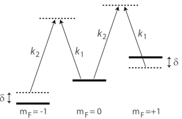
1.1 Illustration of the dressed states of a system in F = 1 hyperfine level, representing the experimental scheme employed by Ref. [1]. The sublevels are first split by a real magnetic field (dotted lines for mF =±), and then coupled with resonant Raman transitions

k1,2. Then a second, position-dependent Zeeman shift is applied

(solid lines), creating a spatially changing detuning δ(r). So, the energy of the dressed states will change with position, and a par-ticle adiabatically following such a dressed state will experience a geometric phase. . . 4 2.1 A simple illustration of the system. N − 1 uncharged fermions

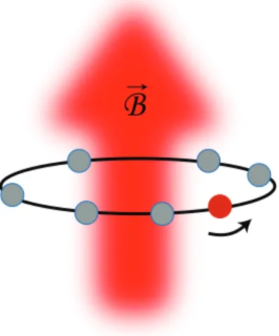
(light gray) and a single charged impurity (dark gray) are trapped on a ring. The impurity is interacting with the fermions via Delta-function interaction. An AMF couples exclusively to the impurity. The dynamics of the system depends on the interaction strength between particles and the total flux through the ring β = qRA_~ .

c

⃝2015 APS . . . 10

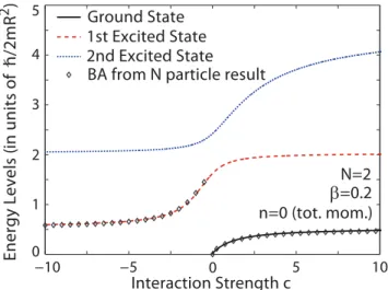
2.2 Energy of the three lowest states vs. interaction strength for

N = 2 particles, and zero total angular momentum. Only

scat-tering states are displayed. Energy is calculated in three diﬀerent ways. Lines are from Eq.2.19 direct analytical solution without employing BA, which is algebraically same as the two-particle BA calculation (Eq.2.18). Diamonds are from the general N -particle BA calculation (Eq.2.27). c⃝2015 APS . . . 15

(9)

LIST OF FIGURES ix

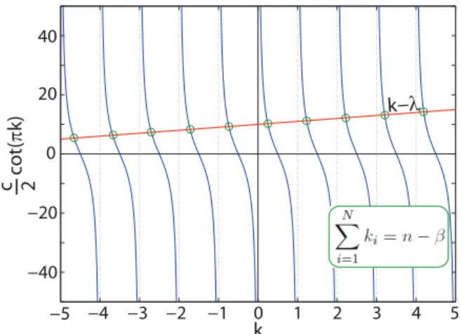
2.3 A representation of graphical solution to BA equation. The cot πk term in Eq.2.27 diverges at every integer k and there is a root between every consecutive integer independently from λ(β). By changing the value of λ, all roots can be adjusted so that the total angular momentum constraint is satisfied. c⃝2015 APS . . . 19 2.4 Ground state energy vs. flux β for N = 2 particles with total

angular momentum n. Eigenstates for flux β with total angular momentum n are also eigenstates for flux β + 1 with total angular momentum n + 1. The system can be analyzed by considering flux values between −1/2 < β < 1/2 for all n. As the flux is increased by one adiabatically, the system evolves to a higher excited state which has one more unit of total angular momentum. The cross-ings between diﬀerent eigenstates is not a problem for adiabatic evolution since only states with diﬀerent total angular momentum

n are degenerate. c⃝2015 APS . . . 20

2.5 Ground state energy vs. interaction strength for N = 1000 parti-cles and zero total angular momentum. Numerical solution of BA equation Eq.2.27 (dots) are virtually indistinguishable from ana-lytical solution (circles) E =(Fermi energy of N−1 fermions)+∆E. Error between the numerical and analytical solutions are too small to observe even in the regimes where the assumptions for analytical calculation fails. c⃝2015 APS . . . 23 2.6 Angular momentum of the impurity vs. interaction strength for

N = 100 particles for (a) attractive and (b) repulsive

interac-tions from the analytic calculation; numerical soluinterac-tions produce the same results. In the non-interacting limit, the impurity carries all the angular momentum (n− β). L1 saturates to zero for

in-finitely strong repulsive interactions as the total angular momen-tum is shared equally between all particles. The same behavior holds for excited states. For strongly attractive interactions, L1

saturates to half the total value, signifying dimer formation with one background particle. The insets in both figures focus on the weak interaction limit. c⃝2015 APS . . . 25

(10)

LIST OF FIGURES x

2.7 The angular momentum of the charged particle vs. flux at vary-ing interaction strength for N = 100 particles. As expected L1

depends linearly on flux. The slope of the line decreases with in-creasing interaction strength indicating higher values of eﬀective mass of the impurity. c⃝2015 APS . . . 26 2.8 Eﬀective mass of the impurity vs. interaction strength for N = 50

particles and zero total angular momentum n = 0. (a) For attrac-tive interactions, m∗ saturates to twice the mass of the impurity due to the formation of a tightly bound pair. The inset shows the behavior around zero interaction in more detail. For attractive interactions, the eﬀective mass (given by Eq.2.39) is almost insen-sitive to flux change. (b) For repulsive interactions, m∗ converges to N . As flux β increases, this saturation gets faster. The depen-dence on the flux is more prominent for small particle numbers.

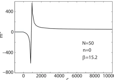
c

⃝2015 APS . . . 27 2.9 Resonant behavior in m∗ for β comparable to N . When the

drag-ging eﬀect of the background particles overcomes the driving force of the magnetic field, m∗ can become negative. When the sec-ond derivative of the energy with respect to flux becomes zero,

m∗ diverges. This divergence does not alter the infinitely-strong interaction limit. c⃝2015 APS . . . 28 2.10 Eﬀective momentum density in k-space for diﬀerent interaction

strengths. In the strongly interacting limit, the distance between adjacent BA roots (wavevectors) is one. For small c, the roots are closer to each other around (n− β), which means the impurity carrying n− β units of angular momentum in the non-interacting limit first disturbs the fermions which are momentum matched to that value. c⃝2015 APS . . . 29

(11)

LIST OF FIGURES xi

2.11 Two-particle correlation function for N = 2 particles. As ex-pected, g12 at zero separation decreases with increasing

interac-tion strength. For weak interacinterac-tions, the correlainterac-tion funcinterac-tion at zero decreases with increasing flux. However, for strong interac-tions, the correlation is almost insensitive to flux change due to the fermionization of the charged particle. c⃝2015 APS . . . 31 2.12 Two-particle correlation function for N = 50 particles. (a) For

weak interactions, Friedel oscillations occur as interference of two waves with wavelengths related to kF−β and kF+β. (b) At strong

interactions, the correlation becomes zero at zero separation since the impurity is eﬀectively indistinguishable and g12 and the

fre-quency of Friedel oscillations are almost insensitive to flux change. c

⃝2015 APS . . . 32

2.13 Kinetic energy of the particles vs. interaction strength for β = 0.2 and β = 10.2 for N = 50 particles. The inset shows the interaction potential contribution to the total energy. The initial increase in interaction energy follows the increase in the interaction strength. However, beyond a certain strength, the tendency of the fermions to avoid the impurity is more dominant. These plots are obtained by taking the derivative of the total energy with respect to c. Alternatively, the interaction potential energy is also obtained by using the two-particle correlation function at zero separation. Both results are plotted in the inset showing remarkable agreement.

c

⃝2015 APS . . . 34

3.1 Superconducting phase diagram. For weak magnetic fields, semi-classical approximation predicts monotonically decreasing critical temperature TC (dashed line). For strong magnetic fields, one must

consider the Landau level structure. A fully quantum mechanical treatment shows oscillations in TC at high magnetic fields,

(12)

LIST OF FIGURES xii

3.2 Phase diagram of the system as a function of dimensionless tem-perature ˜T = kBT /~ω and eﬀective density n1 = N π2ℓ3 where N

is the real-space density and ℓ =√~/mω. Notice that increasing AMF, B = mω/√q1q2, corresponds to lower n1 values. Two

fre-quency ratios ωr = 1 and ωr = 0.95 are displayed for the same

interactions strength ˜as = as(N π2)1/3 = 0.53. For ωr = 1, there is

SC transition at any field, the oscillations in TC (stars) originates

from the LL structure. For ωr = 0.95, this oscillation evolves into

bubble SC regions (shaded areas). The system is not SC even at zero temperature between the bubbles and the transition becomes weakly reentrant in temperature. At the low (many LLs) and high field (only LLL) regimes, TC is not aﬀected significantly by a small

charge imbalance. c⃝2016 APS . . . 46 3.3 Pairing susceptibility (left panel) and respective phase diagrams

(right panel) for three frequency ratios ωr = 1, 0.95, 0.75. The

sys-tem is made dimensionless with eﬀective magnetic energy~ω as in Fig.3.2 and decreasing n1 corresponds to increasing AMF at fixed

real-space density N . The phase diagrams are in linear scale in order to cover TC = 0 and plotted for intermediate field strengths

where charge imbalance eﬀects are most prominent. a) Pairing susceptibility of equal charges diverges at low temperature, guar-anteeing SC for any field value. Divergence is more pronounced at LL thresholds. The corresponding phase diagram (b) is obtained by Eq.3.23. The phase boundary is also highlighted on the surface. c) Even a slight asymmetry between the charges, ωr = 0.95, lifts

the low temperature divergences and the oscillations in (b) turn into bubble SC phases (d). Each LL susceptibility peak is split into smaller peaks, thus, the bubble phases branch into smaller bubbles for weaker interactions (not displayed). e,f) The mismatch between LL spectra is greater for smaller ωr, resulting in prominent

reen-trance with temperature. The maximum reenreen-trance temperature is controlled by~|ω1− ω2|. c⃝2016 APS . . . 48

(13)

LIST OF FIGURES xiii

4.1 Non-equilibrium Hall conductivity, Cneq, of a single Dirac cone

following a ramp of the gap from −∆ to ∆ in time 2τ as shown in inset. Cneq is measured in units of e2/h, and the product ∆τ /~

is dimensionless. In the sudden quench limit (τ = 0), Cneq = 1/6

and as ∆τ → ∞, Cneq → 1/2. The dashed line shows prediction

of the LZ theory from Eq.(4.9). c⃝2016 APS . . . 55 4.2 Haldane model. (a) illustrates the matrix elements of the

tight-binding Hamiltonian in Eq.(4.10); hoppings t1, t2e±iϕ and bias 2M

between A (dark) and B (light) sublattices. (b) Phase diagram showing the Chern number of the lowest band C = 0,±1. The arrow indicates the quench studied in the text. Bands touch at a single Dirac point for MC =±t23

√

3 sin ϕ. c⃝2016 APS . . . 57 4.3 Non-equilibrium Hall response of the Haldane model. The energy

oﬀset M is suddenly quenched from Mi = MC + ∆M to Mf =

MC − ∆M, where MC = t23 √

3 sin ϕ is the topological transition point. Here ϕ = 0.6π and t2 = 0.1t1. For small quenches one

reaches the fractional regime in which Cneq → 2/3. c⃝2016 APS . 58

4.4 Nonlinear Hall response Cneq = ∂X/∂I following a quench, for

transverse displacement X resulting from an impulse I. The pa-rameters are adimensionalized by using the unit length of the lat-tice. The system is quenched between states ∆M around the tran-sition point MC as detailed in the text. The Hall response of a

non-equilibrium system saturates to equilibrium result (C = 1 in this case) for large impulse. Linear response regime shrinks for decreasing ∆M . c⃝2016 APS . . . 60 4.5 Haldane strip with armchair termination, for parameters

intro-duced in Fig.4.2(a). Unit cell is given by the shaded area. We label the layers in the finite y-direction. Green (thick vertical) lines represent how nearest- and next-nearest-neighbor hoppings are assigned into these layers to calculate the current density Jℓ.

c

(14)

LIST OF FIGURES xiv

4.6 Equilibrium Hall conductivity of the strip as a function of number of layers in the finite direction. The system is in CI state at M = 0 and M = MC− 0.1, for t2 = 0.1t1 and ϕ = 0.6π. Hall conductivity

approaches to the quantized bulk value as 1/L for increasing strip width. c⃝2016 APS . . . 63 4.7 Eﬀect of a harmonic trap with ~ω = 0.09t1 in the finite direction

for M = 0, t2 = 0.2t1 and ϕ = 0.5π. (a) Local density of states

along the finite direction where the center is a CI and the edges are metallic. The Fermi energy is indicated with the red line. (b) Current density flowing along the strip with (dark line) and with-out (light line) trap, in the absence of an electric field. The force exerted by the trap Fy =−mω2y results in anomalous currents in

the central topological region according to jx = eCFy/h (dashed

(15)

Chapter 1 Introduction

Since the first observation of a Bose-Einstein condensate using rubidium [2] and then sodium [3] atoms, the physics of ultracold atomic gases has advanced tremen-dously. These systems are essentially the quantum emulators of Feynman’s origi-nal idea [4], where an isolated and controllable quantum system is used in simulat-ing other quantum mechanical phenomena arissimulat-ing naturally in condensed matter. Rapid developments in experimental techniques, regarding cooling and probing, have rendered ultracold quantum gases the ideal laboratory to observe many-body physics. Several theoretical models have been observed for the first time in these systems such as the superfluid to Mott transition or the BEC-BCS crossover, and several others challenged by these experimental achievements [5, 6, 7, 8].

The main appeal of the ultracold atomic gases has been the level of control and tunability of the experiments. One can engineer the confining potentials into a desired geometry, choose particle types, create a clean system or add impurities at will, and tune the inter-particle interactions from infinitely-strong attractive to infinitely-strong repulsive limit. The dominant interaction between these atoms is through s-wave scattering which can be tuned via Feshbach resonances between the atoms [9]. On the other hand, the constituents of the cold atom experiments are neutral atoms. Hence, at the first glance, it may seem impossible to observe the eﬀects originating from an external magnetic field. However, one can always

(16)

try working around this problem by mimicking the eﬀect of a magnetic field in the system.

Under a magnetic field, a charged particle performs cyclotron motion and it is possible to create the eﬀect of this Lorentz force artificially. Initial eﬀorts in this direction employed rotation using the analogy with the Coriolis force. However, rotation as a synthetic magnetic field brings further constraints on the confining potential of the ultracold system to keep particles from escaping the harmonic trap at high frequencies and requires perfectly symmetric traps [10].

A recent development in ultracold quantum gases is the creation of geomet-rically induced artificial magnetic fields (AMFs) [11, 12]. This method does not impose any constraint on the symmetries of the underlying system and enables the investigation of orbital magnetism in a wide variety of settings. Classically, the fields (electric, magnetic) are the important quantities, not the potentials. Contrarily, the magnetic field enters into the Hamiltonian in the form of vector potential in quantum mechanics, enabling coupling even if the strength of the magnetic field vanishes at some point in space. When a charged particle moves along a closed loop, the eﬀect of the magnetic field can be characterized in terms of the Aharonov-Bohm (AB) phase that the particle feels. This AB phase is given by the flux enclosed by the loop. In other words, it depends only on the geometry of the contour, not on the dynamics (e.g. the velocity) of the particle while traveling around the loop. One can generalize this concept and say that if a particle acquires a geometric phase over the course of a closed loop, it feels an eﬀective magnetic field.

Light-induced AMFs exploit the relation between the AB phase of a real mag-netic field and the Berry phase of an adiabatic cyclic evolution. Berry phase is a geometric phase which emerges when a particle adiabatically follows a local eigenstate while it moves along a closed contour in the parameter space of the Hamiltonian. We encounter the Berry phase in various systems throughout the condensed matter literature. In the case of the AB eﬀect, the Hamiltonian

H = 1 2m ( ⃗ p− qBx ~c yˆ )2 , (1.1)

(17)

is position dependent and a charged particle moving along a circle in real space acquires a geometric phase.1 _{In a lattice, if one chooses the parameter on which}

the Hamiltonian depends, to be the crystal momentum k, and moves a parti-cle along a closed loop in momentum space, the partiparti-cle acquires a geometric phase. In this case, the curl of Berry connection (the Berry curvature) essen-tially defines a ‘magnetic field in the reciprocal space’. Another example is the position-dependent Hamiltonian

H(⃗r) =−µ.B(⃗r), (1.2)

of a neutral particle with magnetic moment µ moving in a plane perpendicular to a nonuniform magnetic field. The local eigenstates are calculated from the Schr¨odinger equation H|ψm(⃗r(t))⟩ = Em(⃗r(t))|ψm(⃗r(t))⟩. If the particle starts

at ⃗r0 in a local eigenstate |ψm(⃗r0)⟩, and moves in the real space adiabatically

under the nonuniform magnetic field, so that at all times it remains in the local eigenstate|ψm(⃗r(t))⟩. At any time, the wave function acquires a dynamical phase

factor of e−~i

∫t

0d t′Em(⃗r(t)) due to the time evolution. When the particle returns to

its initial position ⃗r0, its wave function is again given by the local eigenstate |ψm(⃗r0)⟩. But, aside from the time-evolution phase factor, let us also allow a

phase factor that might result from the position dependency of the eigenstates,

eiφm|ψ

m(⃗r0)⟩. (1.3)

This geometrical phase factor can be easily calculated by inserting the wave func-tion into the time-dependent Schr¨odinger equation i~∂t|ψm(t)⟩ = H(⃗r(t))|ψm(t)⟩

as [13]

φm =

I

d ⃗r i⟨ψm(⃗r)|∂⃗r|ψm(⃗r)⟩. (1.4)

In a cold atom setting, dressed states play the role of the adiabatic eigenstates. In the original experiment by Lin et al., the NIST group used 87_{Rb F = 1}

hyperfine states [1]. They first applied a real magnetic field to Zeeman split

1_{Here, one must note that to simulate the cyclotron motion resulting from the Lorentz force}

⃗

F = ⃗v× q ⃗B, the crucial ingredient is to have nonvanishing q ⃗B product, not the magnetic field

itself nor the charge. So, for a general coupling appearing in the Hamiltonian in the form of (⃗p− α⃗r)2_{, one can always assign an eﬀective charge q}∗ _{and an eﬀective magnetic field B}∗_{, for}

(18)

m = -1_F m = 0_F m =+1_F δ δ k2 k2 k1 k1

Figure 1.1: Illustration of the dressed states of a system in F = 1 hyperfine level, representing the experimental scheme employed by Ref. [1]. The sublevels are first split by a real magnetic field (dotted lines for mF = ±), and then coupled

with resonant Raman transitions k1,2. Then a second, position-dependent Zeeman

shift is applied (solid lines), creating a spatially changing detuning δ(r). So, the energy of the dressed states will change with position, and a particle adiabatically following such a dressed state will experience a geometric phase.

the sublevels m = 0,±1 and lift the degeneracy. Then, by using oﬀ-resonant Raman lasers, they dressed the atomic energy levels (see Fig. 1.1). The system is initially prepared in the eigenstate with the lowest eigenvalue of this atom-light coupling. The eigenenergies of these atomic dressed states can be made position dependent, by making the Raman coupling position dependent. This can be achieved, for example, by a spatially changing detuning of the laser frequency or a spatially changing laser intensity. The NIST group employed a position-dependent detuning; i.e. along one spatial direction, let us say ˆy, they uniformly

changed the detuning δ between the atomic states and the Raman transitions, which can be easily achieved by implementing a position dependent Zeeman shift for these atomic levels. If the particles move slowly enough, they adiabatically follow the lowest energy dressed state at each y-point in space. Therefore, the position dependence of the eigenstates results in a geometric phase.

Raman-coupling of the internal degrees of freedom of the atoms has facilitated the realization of synthetic gauge fields in various setups, and even been used to create synthetic dimensions [14, 15]. However, all of these AMF experiments have employed only a single atomic species. In this thesis, we point out an im-portant, yet hitherto unexplored, aspect of the AMFs. The techniques described

(19)

above inducing the geometric phases are highly sensitive to the internal degrees of freedom of the atoms. Therefore, if one applies this scheme to a mixture of two different atomic species, or to a mixture of the same species at different hyperfine levels, the resulting coupling will be different for the two components. For exam-ple, the g-factors for87Rb 5S1/2 F = 1 and85Rb 5S1/2 F = 2 have a 3/2 ratio. If

the original recipe implemented by Ref. [1] is to be applied to a mixture of these atoms at diﬀerent hyperfine levels, position dependent detunings, consequently the AMFs, would reflect this ratio.

This unequal coupling to the different components of a system can have non-trivial consequences, testing the limits of orbital magnetism effects, or can be implemented as a probe for the response of the system. In the next chapter, we first consider a one-dimensional Fermi gas trapped in a ring geometry (the results are published in Phys. Rev. A 91, 053625 (2015)). We then drop an atom from another species or hyperfine level among the fermions, and consider an AMF coupling specifically to the impurity atom. When the impurity is inter-acting with the fermionic background, we can pump angular momentum to the fermions by using the AMF. We show that such an AMF is a versatile tool to in-vestigate the impurity dynamics and the polaron formation. Using Bethe Ansatz, we calculate the eigenstates and corresponding energies exactly as a function of the flux passing through the toroidal trap. Adiabatic change of flux connects the ground state to excited states due to flux quantization. We consider contact interactions between the impurity and fermions, and analyze the full spectrum for the interaction strength, from the strong attractive to the infinitely-strong repulsive limit. The impurity atom perturbs the Fermi sea by dragging the fermions whose momentum matches the flux, and this drag transfers momentum from the impurity to the background. Analyzing this angular momentum trans-fer can help us understand the angular momentum transtrans-fer occurring at larger scales between two different species in a mixture which are rotating at different rates. One must also analyze the effect of interactions on the effective mass of the impurity. For attractive interactions, formation of a dimer from the impurity and one fermion can be also investigated in detail by using the AMF.

(20)

condensed matter theory; superconductivity. In the semiclassical approximation, critical temperature of a superconductor decreases with applied magnetic field. However, if one includes the Landau level (LL) structure at high field values, the critical temperature surprisingly starts increasing with some oscillations (see Fig. 3.1). This high-field superconductivity was first predicted by Teˇsanović in 1989 [16]. However, an experimental observation has been elusive due to the high magnetic field values required in a solid state system to confine particles into their first few LLs, not even mentioning the low temperatures required to observe the quantization effects. In Chapter 3, we propose to use light-induced AMFs in cold atoms to investigate the superconducting phase diagram in the strong coupling limit (the results are published in Phys. Rev. Lett. 116, 045305 (2016)). In the cold atom context, two different atomic species or two different hyperfine states would play the role of up and down spins forming the Cooper pairs, and therefore, resulting in an unequal coupling to the AMF. This enables the study of Bardeen-Cooper-Schrieffer (BCS) pairing of fermions with unequal effective charges. This constitutes a fundamental extension of the BCS theory, in addition to the studies on pairing in the presence of density [17, 18] or mass imbalance [19, 20]. We investigate the superconducting phase diagram of a system formed by such pairs of unequal effective charges as a function of field strength. We consider a homogeneous two-component Fermi gas of unequal effective charges with attractive contact interactions. We employ a two-channel model to describe the system and analytically calculate the Gap equation at the transition point.

Finally, aside from mixtures, one can also simulate various condensed matter models by using synthetic gauge fields in the clean environment of cold atoms; such as the topologically protected states which have attracted great interest of the condensed matter community over the last decades. Thouless, Kosterlitz and Haldane were awarded the Nobel Prize in Physics in 2016 for their contribution to the theory of topological phases of matter [21]. The Haldane model is a sim-ple yet realistic topological lattice model which realizes quantum Hall eﬀect in the absence of an external magnetic field [22]. Since its proposal in 1988, the Haldane model has been constantly studied by theorists to investigate topologi-cally protected states of matter. However, its experimental observation has only

(21)

been achieved in a cold atom setting [23], by implementing an AMF in an optical lattice. Recent cold-atom realizations [23, 24, 25, 26, 27, 28] open up the pos-sibility of exploring topological response in diﬀerent limits enabled by the high controllability of the experiments.

Depending on the staggered magnetic field passing through a unit cell, the Haldane model can be either in a topologically trivial state or have ±1 Chern number. Therefore, by suddenly quenching the magnetic field value, one can drive the system across a topological phase boundary. This is something impos-sible to implement in a solid state setting, because a sudden change of a real magnetic field would induce Eddy currents and inevitably heat the system. In cold atoms, however, magnetic fields are created artificially and one can study quenches between Hamiltonians with diﬀerent magnetic field values. In Chapter 4, we theoretically investigate the Hall response of a lattice system following a quench where the topology of a filled band is suddenly changed (the results are published in Phys. Rev. A 94, 053604 (2016)). Aspects of the original topology survive the quench, but most physical observables (edge currents, Hall conductiv-ity) appear to be non-universal. In the limit where the physics is dominated by a single Dirac cone, we find that the change in the Hall conductivity is two-thirds of the quantum of conductivity. We explore this universal behavior in the Haldane model, and discuss cold-atom experiments for its observation.

(22)

Chapter 2 Impurity under an Artificial

Magnetic Field

The dynamics of a single impurity interacting with a many-particle background is one of the central problems of matter physics. Several condensed-matter models can be reduced to a problem of an impurity interacting with a reservoir. Depending on the type of the impurity (magnetic/nonmagnetic, stationary/mobile, charged/neutral ...), the type of the interactions in the sys-tem (contact, dipolar ...), or the specifics of the syssys-tem (fermionic, bosonic, dimensionality ...), a wide range of phenomena can be observed in this setup [29, 30, 31, 32, 33, 34, 35]. Compared to a full-scale many-body problem, the dynamics of an impurity is generally easier to treat where the most interesting physics emerges around the impurity and, hence, can be controlled in a better way. This, however, does not imply that it is trivial. The collective behavior of the system can be quite unconventional as in the Kondo eﬀect [29] or the po-laron formation [31, 35]. Therefore, it is fundamentally important to examine how these novel phenomena emerge from the underlying interactions between the building blocks of the system.

Here, we consider an impurity atom in a cold atom setting. If one creates an artificial magnetic field (AMF) in the system by coupling light to the internal

(23)

states of the atoms, the effect will be highly sensitive to the internal degrees of freedom of the particles. So, the resulting effective magnetic field acting on the impurity atom and the background atoms will be different. We argue that an AMF coupling specifically to the impurity is an efficient way to probe the polaron state.

For the theoretical study of an impurity, one generally resorts to some form of approximation, e.g. by averaging out the eﬀect of the background. An exact solution for a many-body system is rare in the literature. One great example for such an exact solution is the Bethe Ansatz (BA) in one dimension. The BA solution has been generalized to many integrable models, e.g. systems with multiple components, diﬀerent statistics or spin [36, 37, 38, 39, 40]. This exact solution method has been employed to explain experimental data on a number of instances [41, 42]. However, as BA methods are restricted to one dimension, they have not been used to describe systems where an external artificial gauge field is present.

In one dimension, such an external magnetic field can be disregarded by using a gauge transformation, unless the one dimensional system closes onto itself. Thus, if the particles are confined to a ring as opposed to a line segment, the AMF will significantly eﬀect the physics. Such rings, in the form of toroidal traps, have been realized experimentally [43, 44, 45, 46, 47, 48, 49, 50], although none of these experiments have included an artificial gauge field so far. When the radial extent of a toroidal trap is small, so that only a single mode is supported in the radial direction, the system becomes quasi one dimensional and can be treated exactly with BA.

Here, we consider a one-dimensional spin polarized Fermi gas trapped in a ring geometry and drop an impurity atom among them (see Fig. 2.1 for the illustration). In the cold-atom context, both the impurity and the fermions are neutral atoms. Under an AMF coupling exclusively to the impurity, it will act like a charged particle among the uncharged fermions. We imagine an AMF along the axis of ring by the use of which we can pump angular momentum to the system. The charged impurity is expected to drag the uncharged fermions along

(24)

B

Figure 2.1: A simple illustration of the system. N − 1 uncharged fermions (light gray) and a single charged impurity (dark gray) are trapped on a ring. The impurity is interacting with the fermions via Delta-function interaction. An AMF couples exclusively to the impurity. The dynamics of the system depends on the interaction strength between particles and the total flux through the ring β = qRA_~ .

c

⃝2015 APS

with itself around the ring. Because of the interactions between the impurity and the background atoms, a collective excitation usually called a polaron, is formed [51]. This excitation will couple to the external magnetic field with the charge of the impurity particle, however, its mass will critically depend on the interaction strength. The amount of angular momentum carried by the impurity and the uncharged fermions also depend on the total external flux through the ring. By changing the AMF strength, it is possible to access excited states of the system adiabatically. We describe this system exactly using a BA solution for contact interactions, which are justified for cold atoms since the dominant scattering is s-wave, and show that using an AMF coupling the impurity would be a very eﬀective tool to observe the resulting polaron physics.

This chapter is organized as follows: In the next section, we define the model, introduce the notation and review earlier studies. In Section 2.2.1, we solve the system for two particles and then generalize to any particle number using the BA in Sec. 2.2.2. Sec. 2.3 presents the analytical solution of the BA equations in certain limits and the comparison with numerical solutions. We calculate several

(25)

quantities such as energy, angular momentum and eﬀective mass of the charged particle.

The discussion presented in this chapter is based on the material published in Ref. [52].

2.1 The Model

The Schr¨odinger equation for one charged particle under a magnetic field among

N − 1 uncharged fermions of equal mass m reads HΨ = EΨ, 1 2m (~ i ∂ ∂x1 −qA)2−~2 2m N ∑ j=2 ∂2 ∂x2 j +2c N ∑ j=2 δ(x1−xj)Ψ(x1, x2..xN) = EΨ(x1, x2..xN), (2.1) in the first quantized form. All particles are assumed to be on a ring of radius R; 0≤ xi ≤ 2πR. The position of the charged particle is x1 and A is the vector

potential in the symmetric gauge. The impurity interacts with the background atoms with contact interactions of strength c. The Hamiltonian can be adimen-sionalized by using the radius of the ring: ˜xj = x_Rj, ˜E = E2mR

2

~2 , ˜c = c

2mR ~2 and

β = qRA_~ , where β is the total magnetic flux through the ring in units of flux quantum q/h. We then drop the tildes for simplicity, so that the Hamiltonian is given by H =(− i ∂ ∂x1 − β)2 − N ∑ j=2 ∂2 ∂x2 j + 2c N ∑ j=2 δ(x1− xj). (2.2)

The eﬀect of the magnetic field can be shifted to the boundary conditions (Ψ(x1+

2π, x2..xN) = Ψ(x1, x2..xN)) by a gauge transformation [53], e−iβx1_Heiβx1 | {z } H′ e−iβx1_Ψ(x 1, x2..xN) = Ee−iβx1Ψ(x1, x2..xN) (2.3) z }| { [ − N ∑ j=1 ∂_j2+ 2c N ∑ j=2 δ(x1− xj) ] Ψ′(x1, x2..xN) = EΨ′(x1, x2..xN), (2.4)

(26)

where Ψ′ = e−iβx1_{Ψ, and we again drop the prime-sign on Ψ in the following.}

Namely, when the first particle (charged impurity) makes a full circle around the ring the wave function gains a phase factor of eiβ2π _{where the periodic boundary}

conditions (PBCs) for the uncharged particles remain unaﬀected by the gauging process.

Apart from the twisted boundary conditions (BCs), the δ-function interaction serves as two-sided BC between two diﬀerent regions of space which are essentially diﬀerent permutations of particles. This discontinuity relation can be obtained easily by passing to the center of mass (z) and relative coordinates (y),

y = x1− x2 z = x1+x2 2 } ∂1 = ∂y+ 1₂∂z ∂2 =−∂y1 + 1₂∂z } ∂y = 1₂∂1− 1₂∂2 ∂z = ∂1 + ∂2. (2.5)

By integrating the Hamiltonian with respect to the relative coordinate for∫_−ϵ+ϵdy when ϵ→ 0, ∫ 0+ 0− dy → [ − 2∂2 y − 1 2∂ 2 z + 2cδ(y) ] Ψ(y, z) = EΨ(y, z), (2.6) we obtain the two-sided discontinuity relation for contact interactions,

2∂yΨ(y, z)

0+

0−

= 2cδ(y)Ψ(y = 0, z). (2.7)

By going back to normal coordinates, we find the discontinuity relation at the boundary x1 = xj as (∂j − ∂1)ψ x1<xj − (∂j − ∂1)ψ xj<x1 = 2cψ xj=x1 , j ̸= 1. (2.8)

This one-dimensional problem of two-component fermions has been studied by using the BA in the previous century. First, the one-spin deviate problem in a Fermi sea is solved by McGuire [39], then Flicker and Lieb [54] solved the two-spin deviate problem. Yang [38] elegantly derived the BA equations for the general

M down-spins among N up-spins. Twisted BCs have been used throughout the

BA literature as a way to probe ground state properties. However, with the possibility of optically inducing AMFs, it is important to calculate the properties

(27)

of the system at finite flux as opposed to infinitesimal values near zero. It is also necessary to consider cases where diﬀerent components in the system experience diﬀerent gauge fields.

Our calculation takes both of these constraints into account and allows us to exactly study the dynamics resulting from the dragging eﬀect of the charged particle on the uncharged particles. The resulting polaron physics has attracted great interest in the context of cold atoms over the last few years [51, 55].

2.2 The Ansatz

As the interactions are reduced to BCs, the wave function for a given permutation of the particles can be written as a superposition of plane waves. Since the collisions of equal mass particles in one dimension conserve magnitudes of the incoming momenta, the interacting problem is integrable. Hence, in a given region only a finite number of plane waves are needed to construct the wave function. To make our notation clear, we first start with the case of one charged particle with one neutral particle.

2.2.1 N = 2 Particles

For two particles we have 2! = 2 regions and the wave function in these regions is expressed as follows:

R1 : x1 < x2 Ψ12(x1, x2) = (12)12ei(k1x1+k2x2)+ (21)12ei(k2x1+k1x2) (2.9) R2 : x2 < x1 Ψ21(x1, x2) = (12)21ei(k1x1+k2x2)+ (21)21ei(k2x1+k1x2) (2.10)

where we use parenthesis with a subscript to indicate the coeﬃcients of plane waves. In this notation numbers in the parenthesis indicate the order the wave vectors k1, k2are distributed to the coordinates in the exponent and the subscript

indices indicate the ordering of the particles on the ring, i.e. Ψ12 means x1 < x2.

(28)

derivative should obey Eq.2.8. Equating the coeﬃcients of each plane wave on both sides, we obtain:

BCs: at x1 = x2, (12)21+ (21)21 = (12)12+ (21)12, (2.11) (12)21− (21)21 = (12)12 ( 1 + 2 s12 ) + (21)12 ( − 1 + 2 s12 ) , (2.12)

where s12 = i(k1 − k2)/c. Combined BCs (continuity of the wave function and

discontinuity of its derivative) give     (12) (21)     21 =     1 + 1 s12 1 s12 −1 s12 1− 1 s12         (12) (21)     12 . (2.13)

Allowed values for k1, k2 are found by applying the PBCs. PBC for one of the

particles gives the BA equation.

Twisted BCs: at 2π

as x2 : 0→ 2π, Ψ21(x2 = 0) = Ψ12(x2 = 2π),

(12)21= (12)12eik22π, (21)21= (21)12eik12π. (2.14)

as x1 : 0→ 2π, Ψ12(x1 = 0) = eiβ2πΨ21(x1 = 2π),

(12)12 = (12)21ei(k1+β)2π, (21)12 = (21)21ei(k2+β)2π. (2.15)

Combining the two BCs at 2π, we obtain another constraint k1 + k2 + β = n,

for n ∈ Z. This is a reflection of the total angular momentum conservation in the system. Eqs.2.13 and Eq.2.15 have non-trivial solutions only when the determinant below vanishes,

    (12) (21)     21 =     1 + _s1 12 1 s12 −1 s12 1− 1 s12         (12) (21)     12 =     e−i(k1+β)2π₍₁₂₎ 12 e−i(k2+β)2π₍₂₁₎ 12     (2.16)

(29)

0 1 2 3 4 5 _{Ground State} 1st Excited State 2nd Excited State BA from N particle result

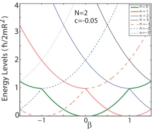
N=2 β=0.2 n=0 (tot. mom.) E n e rg y L e v e ls ( in u n it s o f h /2 m R ) 2 Interaction Strength c −10 −5 0 5 10

Figure 2.2: Energy of the three lowest states vs. interaction strength for N = 2 particles, and zero total angular momentum. Only scattering states are displayed. Energy is calculated in three diﬀerent ways. Lines are from Eq.2.19 direct ana-lytical solution without employing BA, which is algebraically same as the two-particle BA calculation (Eq.2.18). Diamonds are from the general N -two-particle BA calculation (Eq.2.27). c⃝2015 APS

1 + _s1 12 − e −i(k1+β)2π 1 s12 −1 s12 1− 1 s12 − e −i(k2+β)2π = 0. (2.17)

The solution of this determinant gives the BA equation,

α = c 2cot (_π 2(α + n− β) ) + c 2cot (_π 2(α− n + β) ) , (2.18)

where energy is E = (n−β)₂2+α2 for α = k2− k1. For the two-particle case, this

problem can also be solved exactly without using the BA [56],

c = α

(_cos(π(n_{− β))}

sin(πα) − cot(πα) )

. (2.19)

These two equations (Eqs. (2.18) and (2.19)) analytically reproduce each other and the numerical results match perfectly (Fig.2.2).

(30)

2.2.2 N

− 1 Fermions, One Charged Particle

The distinguishable charged particle is denoted again by x1and the wave function

is defined in N ! regions corresponding to diﬀerent permutations [39]. In each one of these regions, the wave function consists of N ! plane waves in its most general form without imposing the antisymmetry between the fermions. As a total, we have N !× N! coeﬃcients: Ψ123... = (123 . . .)123...ei(k1x1+k2x2+k3x3+...)+ (213 . . .)123...ei(k2x1+k1x2+k3x3+...)+ . . . Ψ213... = (123 . . .)213...ei(k1x1+k2x2+k3x3+...)+ (213 . . .)213...ei(k2x1+k1x2+k3x3+...)+ . . . Ψ132... = (123 . . .)132...ei(k1x1+k2x2+k3x3+...)+ (213 . . .)132...ei(k2x1+k1x2+k3x3+...)+ . . . .. . ... (2.20)

where k1, k2, . . . kN are distinct wavenumbers. BCs at x1 = x2 are not eﬀected

by the addition of other fermions at the end of the sequence:     (123 . . .) (213 . . .)     213... =     1 + _s1 12 1 s12 −1 s12 1− 1 s12         (123 . . .) (213 . . .)     123... . (2.21)

BCs at 2π follow the same logic; as x2 : 0→ 2π

Ψ213...N(x2 = 0) = Ψ13...N 2(x2 = 2π),

(123 . . .)213...N = (123 . . .)13...N 2eik22π,

(213 . . .)213...N = (213 . . .)13...N 2eik12π. (2.22)

Number of independent coeﬃcients decreases considerably by requiring antisym-metry upon exchange of fermions. Every coeﬃcient of a plane wave in region

x1 < x3 < x2 < . . . < xN is identical with the coeﬃcient of the same plane

wave in region x1 < x2 < x3 < . . . < xN, i.e. (some permutation)132 =

(the same permutation)123. This can be shown by noticing that at x2 = x3 the

(31)

−(132 . . .)123...N. Fermionic antisymmetry also relates the wave functions in

sep-arate regions; Ψ123...N = −Ψ132...N. As a result, the coeﬃcients only depend on

the position of the charged particle in the order. We can move indistinguishable fermions through one another at will and the N ! regions reduce to N regions.

After this simplification it is easy to combine the BC at a δ-function with the overall PBC.     (123 . . .) (213 . . .)     213...N =     1 + _s1 12 1 s12 −1 s12 1− 1 s12         (123 . . .) (213 . . .)     123...N =     eik22π_{(123 . . .)} 123...N eik12π_{(213 . . .)} 123...N     . (2.23)

The determinant can only vanish if k1 and k2 satisfy, k1−

c

2cot πk1 = k2−

c

2cot πk2. (2.24)

Remember that these conditions are obtained by using the BCs at x1 = x2 and

by using the first two pairs of plane waves in the wave functions (the coeﬃcients in front of the eix1(k1+k2)+ik3x3 _{term). However, there are other plane waves in}

this same BC, e.g. ((231)123 + (321)123)eix1(k2+k3)+ik1x3 term. If we write down

the BCs for these terms, we will obtain relations between other momenta (e.g. between k2 and k3 for the given plane wave). Alternatively, we can obtain the

relations between other momenta by writing the BCs between other particles, for example BCs at x1 = x3. These two approaches produce the same result, and all

the wavenumbers must satisfy

k1− c 2cot πk1 = k2− c 2cot πk2 = k3− c 2cot πk3 = . . . = λ,

where λ is a real constant. This form is equivalent to the usual BA equations [37].

Hence, the N wavenumbers which define an eigenstate must be chosen as N distinct roots of the equation:

k− λ = c

(32)

However, there is another constraint. Applying PBCs sequentially on all particles restricts λ. As x1 : 0→ 2π, Ψ123...N(x1 = 0) = eiβ2πΨ23...N 1(x1 = 2π), (123)123= (123)231ei(β+k1)2π, as x2 : 0→ 2π, (123)231 = (123)312eik22π, as x3 : 0→ 2π, (123)312 = (123)123eik32π, .. . ... In combination: (123 . . .)123...N = ei(k1+k2+...+kN+β)2π(123 . . . N )123...N, (2.26)

reflecting angular momentum conservation: Sum of all the wavenumbers plus the flux must be integer on a ring.

In short, the BA equation is solved by finding N roots of a simple equation (see Fig. 2.3) subject to the angular momentum constraint:

k− λ = c 2cot πk, N ∑ j kj = n− β, n ∈ Z. (2.27)

So far our treatment implicitly assumed repulsive interactions. In which case, all the wavevectors kiare real. The ansatz can easily be extended to attractive

inter-actions yielding exactly the same equations Eq.2.27 [57]. However, for negative c two of the roots will be complex, as the δ-potential in one dimension has only a single bound state.

2.3 Solution of the BA Equation

The cot πk term in Eq.2.27 diverges at every integer k, thus, regardless of the value of β (or λ) there is a root between every consecutive integer (Fig.2.3). By changing the value of λ, all roots can be adjusted so that the total angular

(33)

−5 −4 −3 −2 −1 0 1 2 3 4 5 −40 −20 0 20 40 k c cot( 2 π k) k−λ

Figure 2.3: A representation of graphical solution to BA equation. The cot πk term in Eq.2.27 diverges at every integer k and there is a root between every consecutive integer independently from λ(β). By changing the value of λ, all roots can be adjusted so that the total angular momentum constraint is satisfied.

c

⃝2015 APS

momentum constraint is satisfied. All the eigenstates in this problem can be labeled identically by choosing N distinct integers corresponding to the diﬀerent branches of cot πk and the total angular momentum n ∈ Z. The energy of an eigenstate is simply the sum of squares of all wavenumbers

E =

N

∑

i=1

k2_i. (2.28)

For the simplest case of β = 0, the ground state corresponds to λ = 0 and the total angular momentum n = 0. The roots k are distributed symmetrically around zero for even N, hence, automatically satisfy the total angular momentum condition. The wavevectors for the ground state are in the N branches of cot from −N/2 to N/2. Excitations above this ground state can be generated by two procedures. First, by changing λ, N roots which are on the same branches of

cot can be generated so as to create an eigenfunction with non-zero total angular

momentum (n ̸= 0). Second, at least one of the roots can be chosen to reside on a branch that is not occupied for the ground state. For such a particle-hole excitation, λ must be adjusted to ensure the total angular momentum constraint.

(34)

−1 0 1 0 1 2 3 4 β = 0 = 1 = 2 =−1 =−2 = 3 =−3 n n n n n n n c=-0.05 N=2 E n e rg y L e v e ls ( h /2 m R ) 2

Figure 2.4: Ground state energy vs. flux β for N = 2 particles with total angular momentum n. Eigenstates for flux β with total angular momentum n are also eigenstates for flux β + 1 with total angular momentum n + 1. The system can be analyzed by considering flux values between−1/2 < β < 1/2 for all n. As the flux is increased by one adiabatically, the system evolves to a higher excited state which has one more unit of total angular momentum. The crossings between diﬀerent eigenstates is not a problem for adiabatic evolution since only states with diﬀerent total angular momentum n are degenerate. c⃝2015 APS

Inclusion of the magnetic field aﬀects only the total angular momentum con-straint. As that constraint is defined only up to an integer (n), the problems with values of β diﬀering by an integer are identical. Eigenstates for flux β which have total angular momentum n are also eigenstates for flux β + 1 which have total angular momentum n + 1. This is a restatement of flux quantization. We can analyze the system by considering flux values between−1/2 < β < 1/2.

However, in an experimental setting slowly increasing the value of the flux through the ring is a useful method to access excited states. As the flux is increased adiabatically from zero to one, the ground state evolves to an eigenstate which has its roots exactly in the same branches as the ground state, but, has a total angular momentum of minus one at zero flux (Fig.2.4). The crossings between different eigenstates do not pose a problem for adiabatic evolution as only states with different total angular momentum n can be degenerate in energy. The BA equation Eq.2.27 can be very efficiently solved once the regions for the roots are determined. We used the Newton-Raphson algorithm to find a solution

(35)

within a particular region. As all the roots depend monotonically on λ, another Newton-Raphson search is employed to satisfy the total angular momentum con-dition. We have found numerical solutions for systems of up to 10000 particles with high accuracy.

Although numerically solving the BA equation is eﬃcient and accurate, an analytic solution can provide more insight about the physics of the system. An-alytic formulae for energy, angular momentum and eﬀective mass also would be desirable to make correspondence with experimental observations.

In the limit of strong interactions 1/c≪ 1 and large particle number N/c ≫ 1, such an analytic form can be obtained by approximating the roots of the BA equation. In this limit, because the cot diverges quickly near integers, most of the roots are close to integers. Apart from the few roots near k ∼ λ, if we say that the s-th positive root occur at ks= s + ∆ where ∆ is small, the BA equation

follows 2 c(s + ∆− λ) = cot (sπ + ∆π) =⇒ ∆ ≈ 1 π cot −1 2 c(s− λ), (2.29)

where ∆/c term is extremely small and omitted. So, we find that the roots occur at k+_s = s + 1 πacot 2 c(s− λ), k−_s = −s − 1 πacot 2 c(s + λ), s = 0, 1, . . . , N 2 − 1, (2.30)

where acot is defined in the continuous region (0, π) for Eqs.2.30 to be accurate guesses. Here we have restricted s to analyze the ground state and excited states with roots on the same cot branches. Applying the total angular momentum

(36)

condition we get, n− β = N/2_∑−1 s=0 ks = 1 π N/2_∑−1 s ( acot2 c(s− λ) − acot 2 c(s + λ) ) = c 2π ∫ xF 0 dx ( acot(x− b) − acot(x + b) ) = −c 2π ∫ xF+b xF−b dxacotx +cb 2, (2.31)

with b = 2λ/c and xF = kF/c = (N − 1/2)/c. Here the initial assumption of

strong interactions and large particle numbers allow us to approximate the sum by an integral. For the ground state and the first few excited states n−β is small compared to N and the integral can be approximated by using N/c≫ 1 as

n− β = c 2π ∫ xF+b xF−b dx atanx≈ cb πatanxF. (2.32)

Through this relation b, hence λ, is obtained for any flux value, allowing us to find expressions for all the roots in a self consistent way.

2.3.1 Energy

Using these expressions for the roots, the total energy can be calculated as

E = N/2_∑−1 s=0 k2_s = N/2_∑−1 s { 2s2+ 2s π ( acot2 c(s− λ) + acot 2 c(s + λ) ) +1 π2 ( (acot2 c(s− λ)) 2 + (acot2 c(s + λ)) 2)} . (2.33)

The first term above is the total ground state energy of N − 1 non-interacting fermions. Interactions result in the second and third terms which are first and second order corrections in our expansion. When ∆’s are small, the third term is

(37)

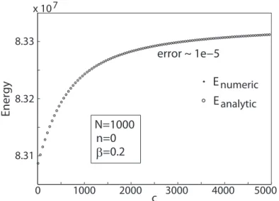
0 1000 2000 3000 4000 5000 8.31 8.32 8.33 x 107 E_numeric E_analytic N=1000 n=0 β=0.2 error ~ 1e−5 c E nergy

Figure 2.5: Ground state energy vs. interaction strength for N = 1000 particles and zero total angular momentum. Numerical solution of BA equation Eq.2.27 (dots) are virtually indistinguishable from analytical solution (circles) E =(Fermi energy of N − 1 fermions)+∆E. Error between the numerical and analytical solutions are too small to observe even in the regimes where the assumptions for analytical calculation fails. c⃝2015 APS

negligible. In this limit, the energy shift due to repulsive interactions (c > 0) is:

∆E = c 2 2π ∫ xF 0 dx x ( acot(x− b) + acot(x + b) ) = c 2 2π { ∫ xF−b −b dx x acot x + ∫ xF+b b dx x acot x + b ( ∫ xF−b −b dx acot x− ∫ xF+b b dx acot x | {z } )} 2π c (n− β) = cb(n− β) + c 2_x2 F 4 − c2 2π ∫ b+xF b−xF dx xatan x = cb(n− β) + c 2_x2 F 4 − c2 4π {( (xF + b)2+ 1 ) atan(xF + b) + ( (xF − b)2+ 1 ) atan(xF − b) − 2xF } ,(2.34) with b = π(n− β) c atan(xF) .

(38)

This approximate form for energy successfully reproduces numeric results for particle numbers as small as 4 throughout all the interaction range. Ground state energy as a function of interaction strength is plotted for a typical case in Fig.2.5 for 1000 particles at β = 0.2 flux. The deviation between numerical and analytical results are too small to observe in this plot.

For attractive interactions, the δ-function interaction supports one bound state in one dimension. Corresponding imaginary wavevectors appear as solutions of the BA equation. For k = α + iσ with (α, σ)∈ R, the BA equation has only two roots with σ̸= 0. The charged particle is bound with only one of the background fermions. When 1/|c| ≪ 1, the complex roots are at k = λ ± ic/2 while the rest of the roots preserve their form given in Eqs.2.30. Within these approximations, we analytically calculate the total energy for attractive interactions,

∆E = −c 2_(b2_{+ 1)} 2 + cb(n− β) + c2_x2 F 4 (2.35) +c 2 4π {( (xF + b)2 + 1 ) atan(xF + b) + ( (xF − b)2+ 1 ) atan(xF − b) − 2xF } , with b = (n− β) c ( 1−_π1atan(xF) ).

If the bound state is narrow, Pauli repulsion between the fermion in the bound pair and background fermions decreases the eﬀective interaction.

2.3.2 Angular Momentum

To understand the physics of the polaron formation and make correspondence to possible experiments, it is important to calculate other measurable quantities. In particular, for this system we are interested in how the dynamics of the impurity particle is aﬀected by the fermion background. To this end, it is instructive to calculate angular momentum carried by the impurity L1 and the related eﬀective

(39)

−10000 −8000 −6000 −4000 −2000 0 −0. 2 −0.15 −0.1 c L1 N=100 n=0 β=0.2 −50 0 −0.2 −0.19 −0.18 c L1 (a) Attractve 0 1000 2000 3000 4000 5000 −0.2 −0.1 0 c L1 N=100 n=0 β=0.2 0 50 −0.2 −0.19 −0.18 c L1 (b) Repulsve

Figure 2.6: Angular momentum of the impurity vs. interaction strength for N = 100 particles for (a) attractive and (b) repulsive interactions from the analytic calculation; numerical solutions produce the same results. In the non-interacting limit, the impurity carries all the angular momentum (n− β). L1 saturates to

zero for infinitely strong repulsive interactions as the total angular momentum is shared equally between all particles. The same behavior holds for excited states. For strongly attractive interactions, L1saturates to half the total value, signifying

dimer formation with one background particle. The insets in both figures focus on the weak interaction limit. c⃝2015 APS

only the mass of the impurity, but, also gets a contribution from the fermions dragged along with it. Such a compound object is generally called the polaron state or dimer state especially for attractive interactions.

As stated above, one of the most physically interesting quantities in this system is the angular momentum carried by the charged particle, represented by the operator ˆP1 = −i_∂x∂₁. As this particle is coupled to the external magnetic field,

ˆ

P1 is the canonical momentum not the kinetic momentum. However, canonical

momentum is the quantity that is generally measured by expansion imaging in AMF experiments in cold atoms. The expectation value of ⟨ ˆP1⟩ = L1 is easily

obtained by taking the derivative of the total energy with respect to flux,

L1 = −1

2

∂∆E

∂β . (2.36)

Using the approximate form for the energy Eq.2.34, we obtain

L1 = π(n− β) atanxF − c 4atanxF { (xF+b)atan(xF + b)−(xF−b)atan(xF − b) } . (2.37)

(40)

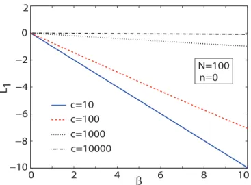
0 2 4 6 8 10 −10 −8 −6 −4 −2 0 2 β L1 c=10 c=100 c=1000 c=10000 N=100 n=0

Figure 2.7: The angular momentum of the charged particle vs. flux at varying interaction strength for N = 100 particles. As expected L1 depends linearly

on flux. The slope of the line decreases with increasing interaction strength indicating higher values of eﬀective mass of the impurity. c⃝2015 APS

This form is valid for positive c and easy to interpret. In the non-interacting limit, the canonical momentum of the charged particle is fixed by the external flux. Hence, all the angular momentum is carried by the charged particle. As in-teractions are turned on, the charged particle drags the background fermions and transfers some of its angular momentum to them. Stronger interactions increase the fraction of the transferred angular momentum, and in the limit of infinitely re-pulsive interactions, angular momentum is equally shared by N particles. On the other hand, for strong attractive interactions, L1 saturates to half of the angular

momentum in the system proving the formation of a dimer with one background fermion.

The behavior of L1 is displayed in Fig.2.6 and Fig.2.7 as a function of

inter-action strength c and flux β. Even for N = 100 particles, the diﬀerence between numerical calculation of the derivative and the expression given above is neg-ligible. As a function of interaction strength, the rapid decrease and eventual saturation of L1 validates the scenario discussed above. The linear dependence

on flux is expected, however, the slope of L1 decreases as interaction gets stronger.

This slope carries valuable information as it is related to the eﬀective mass of the composite excitation formed by the impurity and background fermions.