Effects of endogenous depreciation on the optimal timing of technology adoption

EFFECTS OF ENDOGENOUS DEPRECIATION ON

THE OPTIMAL TIMING OF TECHNOLOGY

ADOPTION

A Master’s Thesis

by

Ramazan Kara¸sahin

Department of

Economics

Bilkent University

Ankara

September 2006

EFFECTS OF ENDOGENOUS DEPRECIATION ON

THE OPTIMAL TIMING OF TECHNOLOGY

ADOPTION

The Institute of Economics and Social Sciences

of

Bilkent University

by

Ramazan Kara¸sahin

In Partial Fulfillment of the Requirements for the degree

of

Master of Arts

in

The Department of Economics

Bilkent University

Ankara

I certify that I have read this thesis and have found that it is fully adequate, in scope and in quality, as a thesis for the degree of Master of Arts in Economics.

Asst. Prof. Dr. H¨useyin C¸ a˘grı Sa˘glam Supervisor

I certify that I have read this thesis and have found that it is fully adequate, in scope and in quality, as a thesis for the degree of Master of Arts in Economics.

Asst. Prof. Dr. Refet G¨urkaynak Examining Committee Member

I certify that I have read this thesis and have found that it is fully adequate, in scope and in quality, as a thesis for the degree of Master of Arts in Economics.

Asst. Prof. Dr. Emre Alper Yıldırım Examining Committee Member

Approval of the Institute of Economics and Social Sciences:

Prof. Dr. Erdal Erel Director

ABSTRACT

EFFECTS OF ENDOGENOUS DEPRECIATION ON

THE OPTIMAL TIMING OF TECHNOLOGY

ADOPTION

Ramazan Kara¸sahin

M.A. , Department of Economics

Supervisor: Asst. Prof. Dr. H¨useyin C¸ a˘grı Sa˘glam September 2006

In this thesis, we use two stage optimal control techniques to analyze optimal timing of technology adoption under embodied technical change taking into ac-count the endogenous nature of depreciation. We show that a more efficient maintenance service reducing the depreciation rate postpones the optimal timing of technology adoption. In this respect, we study to what extent can maintenance of the existing capital stock be a substitute for adoption of new technologies.

Keywords: technology adoption, two stage optimal control, maintenance, invest-ment.

¨

OZET

BAKIM ONARIM HARCAMALARININ TEKNOLOJ˙I

ADAPTASYONUNUN OPT˙IMAL ZAMANLAMASINA

ETK˙IS˙I

Ramazan Kara¸sahin Y¨uksek Lisans, ˙Iktisat B¨ol¨um¨u

Tez Y¨oneticisi: Yrd. Do¸c. Dr. H¨useyin C¸ a˘grı Sa˘glam Eyl¨ul 2006

Bu tezde iki a¸samalı optimal kontrol tekniklerini kullanarak somutla¸stırılmı¸s bir teknik ilerleme ortamında teknoloji adaptasyonunun optimal zamanlaması soru-nunu, a¸sınma payının i¸csel yapısını dikkate alarak ¸c¨oz¨uyoruz. A¸sınma payını d¨u¸s¨urmede daha etkin bir bakım onarım servisinin teknoloji adaptasyonunun op-timal zamanlamasını erteledi˘gini g¨osteriyoruz. Bu ba˘glamda var olan ekipmanın bakım onarımının yeni teknolojilere yapılacak yatırıma ne derecede bir ikame olabilece˘gini inceliyoruz.

Anahtar s¨ozc¨ukler : teknoloji adaptasyonu, bakım onarım, yatırım, iki a¸samalı optimal kontrol.

Acknowledgements

First of all, I want to thank my thesis advisor, H¨useyin C¸ a˘grı Sa˘glam for not only his strong assistance but also for his contribution to my understanding for an ideal academician.

I also especially thank Emre Per, Aslı G¨u¸cl¨ukan and S¨uleyman Tek for their support in the preparation of the thesis.

My dear friends Abd¨ulkadir Bahar, H¨useyin Acan, Yasir Yılmaz, Alperen Uyar and Serkan Y¨uksel all deserve a special thank for their morale support in the last two years.

Lastly and most importantly, I thank my mother and sister for everything I have up to this point in my life. Your existence and love give me the necessary energy for my life.

Contents

1 INTRODUCTION 1

2 BENCHMARK MODEL 5

2.1 Two-stage optimal control approach . . . 7 2.2 Solving the model . . . 9

3 INCREASING FRONTIER TECHNOLOGY CASE 14

3.1 Without Maintenance Control . . . 14 3.2 With Maintenance Control . . . 18

4 NUMERICAL ANALYSIS 21

Chapter 1

INTRODUCTION

Technology adoption has been one of the most important research topics in recent years in macroeconomic studies. With his seminal study, Solow (1956) concluded that the increase in the technological level of the economy is the only way of guaranteeing the long term GDP per capita growth. However the adoption costs have a considerable weight (see Jovanovic, 1997) and this makes technology adoption an interesting research area.

To better understand the costs of technology adoption, consider an economy that realizes technology adoption. In order to adopt the technology, some spe-cific physical and human capital is required. As Parente (1994) states, when technology upgrades, the preexisting human capital has efficiency loss due to the new technology. The labor resources need time in order to gain expertise on the new technology. Such a cost associated with technology adoption has been called learning cost in the existing literature.

Different scholars, considering the benefits and costs of technology adoption, have analyzed the determinants of technology adoption process. Growth ad-vantages of switching, speed of learning and obsolescence costs are shown to be the main determinants of technology adoption by Boucekkine, Saglam and Vallee (2002). Even at the firm level, when the firms demonstrate greater ability in learning, they more frequently adopt higher technologies and will have more market values even if they have lower profitability according to Ahn (2003). The growth rate of the frontier technology level also increases the number of technol-ogy adoptions and shortens the durations between these subsequent adoptions according to Saglam (2002).

Besides these factors, with their empirical study on cross-country technology adoption of more than twenty technologies from 1788 to 2001, Comin and Hobjin (2003) state that the most crucial determinants for technology adoption are real income, human capital, adoption of preceding technologies, openness to trade and the type of the government. The real income is also shown to affect technology adoption decision by Khan and Ravikumar (2000). Poorer households, which start with a smaller level of capital stock are found to postpone adoption to later dates.

Nevertheless, in these studies maintenance activities are not taken into ac-count in the technology adoption analysis. Like most of the optimal growth theories, these studies treat depreciation as constant and build their models with this approach. However, there is enough empirical evidence to conclude that the depreciation rate is not constant and affected by different factors (See Storchmann 2004, Gylfason and Zoega 2001, Mullen and Williams 2004). A well-known al-ternative to constant depreciation is depreciation in use hypothesis, which states that a higher level of economic activity causes a higher depreciation rate. However as Boucekkine, Martinez and Del Rio (2005) state, this hypothesis does not seem to be completely satisfactory. This is the first problem that will be addressed in this paper: How rational is to take the depreciation rates constant in the opti-mal growth models? Taking into account the embodied nature of technological progress, what are determinants of optimal maintenance and depreciation deci-sions? In this analysis, rather than using capital utilization to break the constant depreciation assumption, we will concentrate on the fact that depreciation rate depends on heavily the maintenance services. (See Mullen and Williams 2004, Nelson and Caputo 1997, Nickell 1975). In fact, maintenance spending has been a comparable part of the GDP. For instance, McGrattan and Schmitz (1999) find that maintenance spending is around 6 percent of the GDP for Canada where they also claim that maintenance and investment spending are gross substitutes to some extent.

The most trivial connection between the maintenance and adoption is that maintenance activities use the physical and human resources that can be used for

adoption or investment. In this sense, they compete for taking the resources ex-isting in the economy. Another reason for connecting adoption and maintenance is that while adopting the higher technology, countries or firms also consider the necessary maintenance spending related with this higher technology. If the new capital stock embodying a superior technology will cause an enormous increase in the maintenance spending, the decision to adopt this superior technology can be discarded. This is the second problem that will be addressed in this paper. We will analyze the role of maintenance in the adoption process and try to es-tablish the mechanism that connects the investment and maintenance activities. Can maintenance of the existing capital stock be a substitute for investment in new technologies? If so, to what extent? Can maintenance services provide an alternative explanation for why are the new technologies adopted after a time lag? These questions become increasingly crucial in understanding the optimal timing of technology adoption if one takes into account the embodied technolog-ical progress. As Greenwood, Hercowitz and Krussel (1997) have found, around 60 percent of US productivity growth can be attributed to the embodied techno-logical change.

In this paper, we provide the needed analysis on the role of maintenance in the technology adoption process. Among very few contributions on the role of main-tenance in macro theory, Boucekkine, Martinez and Saglam (2001) characterize the balanced growth paths of their models both with and without maintenance options. As a result they find that although the maintenance option increases the technological gap since the labor resources are diverted from adoption, in the long run the output level increases with the maintenance option. Secondly, they find that the equilibrium maintenance and adoption decisions move in opposite directions for different policy or technology shocks.

At the firm level, Ruiz-Tamarit and Boucekkine (2001) concentrate on the relationship between maintenance and investment activities. They conclude that that investment and maintenance activities are gross complements rather than substitutes. However, their analysis does not take into account the embodied nature of technological progress and is not able to address whether maintenance can act as a substitute for the adoption of new technologies.

The organization of the paper is as follows. In Chapter 2, the benchmark model will be intoduced and solved with the two-stage optimal control approach of Tomiyama and Rossana (1989). The solution procedure of two-stage optimal control will also be clearly established in Chapter 2. In Chapter 3, we will extend our model by allowing the frontier technological level to increase throughout time. However, in Chapter 3, due to the complexity of the model, the open form solutions for the optimal adoption timing cannot be reached as the most of optimal adoption timing analyses. Thus, in Chapter 4, numerical analysis and comparative statistics will take place. The thesis will end with a brief conclusion.

Chapter 2

BENCHMARK MODEL

Our economy consists of a representative agent which has an intertemporal

utility function _Z

∞

0

u(C(t))e−ρt_dt.

Here u(t) is assumed to be increasing and strictly concave. Throughout the paper, we will not analyze the labor dynamics, so for all of the paper we normalize the population to 1 and assume that there is no population growth. Our time horizon is infinite and we also have the discounting parameter ρ as usual. For the consumption sector, our production function is Ak where k(t) denotes the capital stock at time t and A denotes the overall efficiency in the production. The produced good can be used in three alternative ways: it is either consumed, used for investment or used for maintenance activities(We skip time subscripts wherever there is no confusion):

Y = C + I + M = F (k) = Ak

The capital stock in the overall economy evolves according to the following equation:

˙k = qI − δk = (qi − δ)k.

From this point on the lowercase i and m will denote the investment and maintenance spending per capital stock. In the capital stock evolution function q measures the efficiency of the investment and the technological progress is em-bodied with this variable. Unlike A, a rise in this variable will only affect the newest capital goods and investment specific. For the capital stock, we assume

that the initial level of capital stock k(0) = K0 is given. The depreciation rate is affected by the maintenance spending throughout the following function:

δ(t) = ¯δ − am(t)b_.

Here ¯δ represents the maximum level of depreciation when there is no main-tenance throughout the economy. Both a and b are positive variables and they together represent the efficiency of the maintenance spending. With increasing the maintenance spending, the depreciation rate can be decreased and by this way the capital stock on hand will be prevented from getting useless for the production.

For our problem, there are two options for the representative agent: (A1, q1)

and (A2, q2). The level of technology which the economy has at initial point is

q1 and the available technology level for the agent to jump is q2. Obviously, q2

needs to be greater than q1 for this technology adoption problem. This simply

means that by switching to the new regime, the investment spending will be more efficient in terms of increasing production. However, to incorporate the expertise loss due to adopting a new technology, the marginal productivity of the capital in the new regime A2 is smaller than the marginal productivity of the capital in the

first regime A1. Thus, the tradeoff between higher technologies but less efficiency

is well reflected via this model.

Now, assume that the economy switches at date t1 to the new technology

regime, obviously the state equation for the capital stock will be different before t1 and after t1. Before adopting the new technology, i.e. when 0 ≤ t ≤ t1 the

evolution will be:

˙k(t) = [q1i(t) − δ(t)]k(t) (2.1)

On the other hand, after adopting the technology, i.e. when t1 ≤ t the

evolu-tion of the capital stock will be:

˙k(t) = [q2i(t) − δ(t)]k(t) (2.2)

As we see, there is a tradeoff between two consecutive regimes. The marginal productivity of the investment is higher in the higher technology regime, however

as the marginal productivity of the capital stock decreases, the total production thus the resources that can be devoted to investment is negatively effected. After building up the model, in the next subsection we will briefly sketch the two-stage optimal control technique.

2.1

Two-stage optimal control approach

The problem of the central planner can be summarized as: maxi,m,t1

Z _∞

0

u(c(t))e−ρt_dt.

Subject to (2.1), (2.2) and K0 given. When we carefully look at the problem,

it is obvious that the objective function can be rewritten as: U(i, m, t1) = Z _t1 0 u(c(t))e−ρtdt + Z _∞ t1 u(c(t))e−ρtdt (2.3)

Since the original problem’s objective function can be separated into two periods and the welfares of the two possible regimes can be added to find the optimal welfare of the original problem, two-stage optimal control approach can be directly applied as it is clearly suitable for our case. The application of two-stage approach first divides the problem into two two-stages and operates as following:

1) The second stage problem: We start by assuming the economy realizes the switch at time t1 and the initial capital stock at time t1 is given as

k(t1) = K1. For this stage the problem is to maximize the total welfare

obtained from this period, i.e. U2(K1, t1) =

R_∞

t1 u(c(t))e

−ρt_{dt, with subject}

to the state equation 2.2. For this stage let us denote the co-state variable as λ2(t), the corresponding Hamiltonian as H2(k, i, m, t, λ2) = −u(c(t))e−ρt+

λ2(t)[q2i(t) − δ(t)]k(t). Assume there exists a maximum for this problem.

Let us denote the maximum welfare obtained in this stage as U∗

2(K1, t1)

and the minimum Hamiltonian as H∗

2) The first stage problem: Now we turn to the first stage of the model and maximize U(C, t1) =

R_t1

0 u(c(t))e−ρtdt + U2∗(K1, t1) with subject to

equa-tion (2.1), K0 given and finally K(t1) = K1 free. To solve this problem

we first need to solve the first stage Pontryagin problem for fixed t1 and

K1. We will denote the co-state variable as λ1(t) and the Hamiltonian as

H1(k, i, m, t, λ1) = −u(c(t))e−ρt+λ1(t)[q1i(t)−δ(t)]k(t). The resulting

min-imum Hamiltonian will be denoted as H∗

1(K1, t1). The most essential point

of the technique is linking the first stage and the second stage. For interior solutions and assuming U2(K1, t1) is twice continuously differentiable in K1

and t1, the optimal K1∗ and t∗1 should satisfy the following equations:

λ1(t∗1) = λ2(t∗1) (2.4)

H∗

1(K1∗, t∗1) = H2∗(K1∗, t∗1) (2.5)

3) For all of the models we study hereafter, U2(K1, t1) is twice continuously

differentiable in K1 and t1. However, although this assumption is satisfied,

it can be the case that equations (2.4) and (2.5) has no solution for a t1

satisfying 0 ≤ t1. In this case there can be two corner solutions possible:

immediate switching and technological sclerosis. If, H∗

1(K0, 0) ≥ H2∗(K0, 0),

t∗

1 = 0 and the economy immediately switches to the new technology regime.

On the other hand, if H∗

1(K0, 0) < H2∗(K0, 0) for every t1 ≥ 0, the economy

never switches to the new technology regime and technological sclerosis occurs.

Here we need to add that linking the first stage and second stage, i.e. the optimality condition changes when adoption timing t1 explicitly affect the

evolu-tion of capital stock or not. In other words, if t1 exists in any of equations (2.1)

and (2.2), then equation (2.5) is not used to find the optimal adoption timing. Instead we use: ∂U∗ 2(K1, t1) ∂t1 = H₁∗(K1, t1) + Z _t1 0 ∂H∗ 1 ∂t1 dt (2.6)

This equation is also same as the following equation by Tomiyama and Rossana(1989): H₂∗(K1, t∗1) − H1∗(K1, t∗1) = Z _t1 0 ∂H∗ 1 ∂t1 dt + Z _∞ t1 ∂H∗ 2 ∂t1 dt (2.7)

After clearly introducing the two-stage optimal control procedure, in the next subsection we will apply this methodology by not getting stuck on the algebraic details.

2.2

Solving the model

We will closely apply the approach defined above for our model. For making the calculations easier, we will take the logarithmic utility function. We start by considering the second stage problem:

maxi,mU2(c, t1) =

Z _∞

t1

ln(c(t))e−ρt_{dt (2.8)}

Subject to K1 given and state equation (2.2). For this problem Hamiltonian is

H2(k, i, m, t, λ2) = −ln(c(t))e−ρt+λ2[q2i(t)k(t)−δ(m(t))k(t)] and we can directly

write first order conditions:

Hi(k, i, m, t, λ2) = e−ρt_k(t c(t) + λ2(t)q2k(t) = 0 (2.9) Hm(k, i, m, t, λ2) = e −ρt_k(t) c(t) − λ2(t)k(t)δ 0_{(m(t)) = 0 (2.10)} − ˙λ2(t) = Hk(k, i, m, t, λ2) = λ2(t)[q2m(t) + δ(m(t)) − q2A2] (2.11) ˙k(t) = Hλ(k, i, m, t, λ2) = [q2i(t) − δ(m(t))]k(t) (2.12)

And the transversality condition:

lim

When we solve (2.9) and (2.10) together, we finally reach that: δ0(m(t)) = −q2 ⇒ m(t) = ¡ab q2 ¢ 1 1−b _{⇒ δ(m(t)) = ¯δ − a}¡ab q2 ¢ b 1−b

Here we see that for the whole period, in this framework the optimal resources allocated to maintenance, thus the depreciation rate does not change and equal to the above values. Then we denote these constant maintenance and depreciation rate as m2 and δ2 respectively. The integration of the necessary conditions from

(2.9) to (2.12) yield the following results: k(t) = e−(q2m2+δ2−q2A2+ρ)t(1 − eρ(t−t1)) −a0ρ + K1e−(q2m2+δ2−q2A2)(t−t1) (2.14) c(t) = − 1 q2a0 e−(q2m2+δ2−q2A2+ρ)t _(2.15) λ2(t) = a0e(q2m2+δ2−q2A2)t (2.16) i(t) = A2− m2 − c(t) k(t) (2.17)

By using transversality condition we find the constant of integration as: a0 = −

1 K1ρ

e−(q2m2+δ2−q2A2+ρ)t1 _(2.18)

By incorporating this constant of integration to the equations, we can find the optimal welfare as:

U∗ 2(K1, t1) = e−ρt1 ρ ¡ ln[K1ρ q2 ] − q2m2+ δ2− q2A2+ ρ ρ ¢ (2.19) As we see the optimal value of the objective function is twice differentiable both with respect to K1 and t1. After solving the second stage, we need to turn

to the first stage and solve the following problem: maxi,m,t1U1(C, t1) =

Z _t1

0

ln(c(t))e−ρt_{dt + U}∗

Obviously subject to state equation (2.1), K0 given and K1 = k(t1) free. We

first treat the problem as K1 and t1 fixed. This allows us to write the first order

conditions of the problem straightforwardly as in the second stage. Solution of these first order conditions yield:

δ0(m(t)) = −q1 ⇒ m1 = ¡ab q1 ¢ 1 1−b _{⇒ δ} 1 = ¯δ − a ¡ab q1 ¢ b 1−b _(2.20) k(t) = e−(q1m1+δ1−q1A1+ρ)t(1 − eρt) −¯a0ρ + K0e−(q1m1+δ1−q1A1)t (2.21) c(t) = − 1 q1¯a0 e−(q1m1+δ1−q1A1+ρ)t _(2.22) λ1(t) = ¯a0e(q1m1+δ1−q1A1)t (2.23) i(t) = A1− m1 − c(t) k(t) (2.24)

After this point, for finding the optimal t1 value, we will use the equations

(2.4) and (2.5). By using equation (2.4), we find the constant of integration for the first stage as:

¯a0 =

e−(q1m1+δ1−q1A1+ρ)t1

K1ρ

Using this result we find the consumption, investment, co-state and capital stock levels for the first period and t1. Finally in order to determine the optimal

t1, we use equation (2.5) and find:

H∗

2(K1, t1)−H1∗(K1, t1) = 0 ⇒ ρ ln(

q2

q1

)+[q1A1−q2A2]+[q2m2+δ2−q1m1−δ1] = 0

From these results it is obvious that there is no interior solution for the model since in the equation t1 does not exist. Therefore under this framework there

can be only corner solutions. If we analyze under which conditions the corner solutions arise, as we stated in the explanation of the two-stage optimal control technique, the solution is either immediately switching or technological sclerosis. If ρ ln(q2

q1) + [q1A1− q2A2] + [q2m2+ δ2− q1m1− δ1] ≤ 0, the economy

immedi-ately switches to the new technology. Otherwise, the economy sticks to the old technology and does not switch.

Let us interpret this analytical result. The increase in the embodied technol-ogy level results with a decrease in the relative price of capital at the date of switch in our model. Thus the consumption goods have higher relative prices in the second stage and the economy reallocates the resources by increasing capital stock and decreasing consumption at the date of switch. This consumption de-crease also causes the welfare dede-crease and this can be expressed as ρ ln(q2

q1) since

the utility function is logarithmic here. This cost can be called as obsolescence cost.

On the other hand, when the economy switches to new regime although the expertise level decreases, the efficiency of capital goods can compensate this loss and even can supply the economy a greater growth rate. The growth advantage of switching can be expressed as q2A2− q1A1.

Besides the obsolescence cost (ρ ln(q2

q1)) and growth advantage of switching

(q2A2− q1A1) we have the additional term (q2m2 + δ2− q1m1 − δ1) when

com-pared with Boucekkine, Saglam and Vallee (2002). When we consider this term carefully, we see that in fact this term reflects the comparative or additional main-tenance cost in terms of capital goods when the switching is realized. When the economy switches and realizes the optimal maintenance spending, the spending in terms of capital goods is q2m2, since instead of spending m2 units of consumption

good, the economy could have increased the capital stock by q2m2 with investing

this spending. Also, with switching the capital stock in the economy depreciates with δ2 and this is also in terms of capital goods. Thus (q2m2+ δ2− q1m1 − δ1)

reflects the comparative maintenance cost of switching. As a result, the economy switches if and only if the growth advantage of switching exceeds the obsolescence cost and comparative maintenance cost of switching.

Together with this result, we also have an important result that will stay un-changed throughout our models. The relationship between maintenance spending and the technology level of the economy can be summarized as:

m(t) =¡ab qt

¢ 1 1−b

This equation shows the relationship between the maintenance spending mt

and the technology level qt. With this equation we reach the following result. If

the depreciation function is convex with respect to maintenance, i.e. b < 1, as accepted by Boucekkine, Saglam and Martinez 2002 (this is the dominant view of the existing literature), then increase in the technology level is followed by a decrease in the maintenance spending since the derivative of maintenance with respect to technology level is negative then. However, if the depreciation function is concave, then they are positively correlated.

This result is extremely important since this issue has gained a great atten-tion especially in the empirical studies. It confirms Storchmann’s finding that the developed countries have a greater depreciation level than the undeveloped countries. The technology level is much greater in developed countries and this increases the maintenance costs in terms of investment. Thus, instead of main-taining their old cars, they buy new cars and with this obsolescence effect, the depreciation gets higher values in developed countries.

Now in order to find an interior solution and analyze the factors affecting the optimal timing of adoption, in the next section we will extend our benchmark model by incorporating technological progress.

Chapter 3

INCREASING FRONTIER

TECHNOLOGY CASE

In our benchmark model, we started with assuming a constant level of higher technology for switching. Absolutely, in real life the situation is quite different. The frontier level of technology also increases with time and the economy can jump to a higher level of technology by waiting.

To include this reality in our model, we assume that the frontier level of technology increases with a constant speed γ, thus the available level of technology the economy can switch equals eγt_{. Thus in this case, the evolution equation of}

the capital stock in the second stage of this model is:

˙k(t) = [eγt1_{i(t) − δ(t)]k(t) (3.1)}

Other assumptions and variables also continue to be valid in this enlarged model. To see the effects of the maintenance option, in the next subsection we firstly solve the model without maintenance option and then incorporate the maintenance to our model.

3.1

Without Maintenance Control

When there is no maintenance, the depreciation is constant at ¯δ. Moreover, without maintenance spending, the resources can be allocated for consumption and investment. Thus, the resource allocation constraint is:

After taking into consideration these changes in the benchmark model, we again start with the second stage. The corresponding Hamiltonian is:

H2(k, c, λ2, t) = −ln(c(t))e−ρt+ λ2[eγt1i(t)k(t) − ¯δk(t)] (3.2)

The solution of the first order conditions and doing the necessary algebraic manipulations we obtain: c(t) = − 1 λ0eγt1 e−(¯δ−eγt1_A2+ρ)t (3.3) k(t) = e−(¯δ−eγt1_A2)t£ K1e(¯δ−eγt1A2)t1 − e−ρt_{− e}−ρt1 λ0ρ ¤ (3.4) λ2(t) = λ0e(¯δ−eγt1A2)t (3.5)

When we solve the transversality condition, we find the constant of integration as:

λ0 = −e

−(¯δ+ρ−eγt1_A2)t1

K1ρ

(3.6) We replace this constant of integration and obtain the optimal consumption, investment, capital stock, maintenance and total welfare obtained in the second period. Later on, we turn to the first stage. As in section 2, we start by assuming K1 and t1 fixed. This allows us to treat the first stage problem as an ordinary

Pontryagin problem. Writing the relevant first order conditions and integrating them gives us the following results for the first stage problem:

c(t) = −_¯1 λ0q1 e−(¯δ−q1A1+ρ)t _(3.7) k(t) = e−(¯δ−q1A1+ρ)t£−1 + e ρt_{(1 + K} 0ρ¯λ0) ρ¯λ0 ¤ (3.8)

λ1(t) = ¯λ0e(¯δ−q1A1)t (3.9)

Now we need to apply the continuity and optimality conditions. The conti-nuity condition is same as the Section 2. Co-state variable and the capital stock cannot have a distinct jump at t1. Thus considering this continuity condition and

using the results we found for the two stages, we find:

¯ λ0 = − e−(¯δ−q1A1+ρ)t1 K1ρ (3.10) K1 = K0e−(ρ+¯δ−q1A1)t1 (3.11)

Finally, in order to find the optimal timing of adoption, we need to apply optimality condition. However, the optimality condition we will apply in this model is different than Section 2. To understand this optimality condition change, let us consider the evolution equation of the capital stack in the second period for the benchmark model and this model respectively:

˙k(t) = [q2i(t) − δ(t)]k(t) (3.12)

˙k(t) = [eγt1_{i(t) − δ(t)]k(t) (3.13)}

As we see, in the benchmark model the capital stock evolution does not depend on t1. On the other hand, equation (3.13) has t1 and here the capital stock

evolution is not independent of t1. In other words, t1 explicitly effects capital

stock evolution and as Tomiyama and Rossana (1989) states, we need to apply equation (2.7) as the optimality condition.

However, when we try to solve this equation we obtain that the optimal t1

should satisfy the following equation: e−ρt1¡2A

2eγt1(γ − ρ) + ρ2ln[e−t1(−A1+ρ+¯δ)K0ρ] − ρ(−2A1+ γ + ρ ln[K0ρe−t1(ρ+¯δ+γ−A1)])

¢

ρ2 = 0

Obviously, this equation has no algebraic solution and thus we need to do numerical analysis and try to see the effects of maintenance and other variables to adoption timing. However, we can prove the existence of a t1 satisfying this

equation.

Proposition 3.1.1 Assume A2 < A1 and γ < ρ < A2. If we normalize q1 = 1,

then there exists a t1 satisfying equation (3.14).

Proof: When we consider left side of equation (3.14), we see a continuous function of t1. When t1 is 0, this function takes the value (2A1−2A2)ρ+(2A_ρ2 2−ρ)γ

and this value is greater than 0 under these assumptions. When t1 is not

equal to 0, this function becomes e−ρt1¡(2A2eγt1(γ−ρ)+2A1ρ−γρ+ρ2γt1

ρ2

¢

. Obviously e−ρt1 and ρ2 are always positive. On the other hand while t

1 goes to infinity,

(2A2eγt1(γ − ρ) + 2A1ρ − γρ + ρ2γt1 goes to minus infinity. Thus for sufficiently

great values of t1, the function takes negative values. Following intermediate

value theorem we can conclude that there exists a t1 where the function takes the

value 0 and obviously for this value of t1, optimality equation (3.14) is satisfied.

¤

To visualize the proof assume γ = 0.02, ρ = 0.04, A1 = 1 and A2 = 0.8.

Now we need to have 2A2eγt1(γ − ρ) + 2A1ρ − γρ + ρ2γt1 = 0. Here ρ2γt1

refers to obsolescence cost and (2A2eγt1(ρ − γ) − 2A1ρ + γρ refers to growth

advantage. In the optimal time of adoption, growth advantage needs to start exceeding obsolescence cost. When we draw the graph, we see that at 0, growth advantage is below obsolescence cost but however as time passes growth advantage increases faster.

— Insert Figure 1 Here—

In the next section we will include maintenance and obtain the condition for optimal timing.

3.2

With Maintenance Control

Unlike section 3.1, the model we will solve when there is maintenance option has the only difference as replacing equation (3.13) instead of equation (3.12). As defined in the two-stage technique, we start with the second period. The corresponding Hamiltonian is:

H2(k, i, m, λ2) = −ln(c(t))e−ρt+ λ2[eγt1i(t)k(t) − δ(m(t))k(t)] (3.15)

Directly writing the first order conditions and doing the necessary algebraic operations yield the following results for the second stage:

c(t) = − 1 λ0eγt1 e−(eγt1_m2+δ2−eγt1_A2+ρ)t (3.16) k(t) = e−(eγt1m2+δ2−A2eγt1)t£_K 1e(eγt1m2+δ2−eγt1A2)t1 − e−ρt_{− e}−ρt1 ρλ0 ¤ (3.17) λ2(t) = λ0e(eγt1m2+δ2−eγt2A2)t (3.18)

Incorporating the transversality condition, we find the constant of integration as: λ0 = −

e−(eγt1_m2+δ2−eγt1_A2+ρ)t1

K1ρ

(3.19)

After solving the second stage problem, now we turn to the first stage problem. With again taking t1 and K1 fixed, we take the first stage problem as ordinary

Pontryagin problem and directly write the first order conditions. Integrating these conditions give us the following results for the first stage:

c(t) = −_¯1 λ0q1 e−(q1m1+δ1−q1A1+ρ)t _(3.20) k(t) = e−(q1m1+δ1−q1A1+ρ)t£−1 + e ρt_{(1 + K} 0ρ¯λ0) ρ¯λ0 ¤ (3.21)

λ1(t) = λ0e(q1m1+δ1−q1A1)t (3.22)

After finding these results, now we need to apply continuity and optimality conditions to find the optimal t1. As usual the continuity condition states that

the capital stock and co-state variable can not have a distinct jump at adoption time. Applying this condition gives us the following:

¯ λ0 = − e(q1m1+δ1−q1A1+ρ)t1 K1ρ (3.23) K1 = K0e−(q1m1+δ1−q1A1+ρ)t1 (3.24)

Finally to find the optimal adoption timing, we need to apply optimality condi-tion. Solving equation (2.7), we find the condition that optimal t1 needs to satisfy

as: 1 −bρ2 · e−ρt1¡_{− (1 − b)(}ab q1 )1−b1 q₁ρ − bρ(A₁q₁− γ) − A₂beγt1(γ − ρ) +eγt1_(abe−γt1₎1−b1 (ρ − bρ + bγ) − bρ2(− ln£K 0ρe−t1(a(1−b)( ab q1) b 1−b_{−A1q1+ρ+δ+γ)}¤ + ln£e−t1(a(1−b)(_q1ab) b 1−b_{−A1q1+ρ+δ)}K₀ρ q1 ¤ )¢ ¸ = 0 (3.25)

Again this equation can not be solved algebraically and we need to do numer-ical analysis. However, before proceeding to numernumer-ical analysis, we need to show the existence of the optimal t1.

Proposition 3.2.1 Assume γ < ρ, A2 ≤ A1 and ρ + (ab)

1

1−b ≤ A₂. Moreover

assume b < 1, i.e. depreciation function is convex. If we normalize q1 = 1, then

there exists a t1 > 0 satisfying equation (3.25).

Proof: When we consider the left side of equation (3.25), we see a continuous function of t1. When t1 equals 0, this function takes the value:

− 1

bρ2[−bρ(A1− A2) − bγ(A2− ρ − (ab)

1 1−b)]

and under these assumptions this value is greater than 0. When t1 does not

equal to 0, with algebraic manipulations it can be shown that the left hand side becomes: − 1 bρ2[−A2b(γ − ρ)e γt1 _{+ e}−bγt1_{1−b (ab)1−b}1 _{(ρ − bρ + bγ) − bρ}2_γt 1− (1 − b)(ab) 1 1−bρ]. Obviously, − 1

bρ2 is always negative. On the other hand, with given assumptions:

lim t1→∞ [−A2b(γ −ρ)eγt1+e −bγt1 1−b (ab) 1 1−b(ρ−bρ+bγ)−bρ2γt₁−(1−b)(ab) 1 1−bρ] = +∞

This simply means that the function takes negative values for sufficiently great values of t1. Following intermediate value theorem, we can conclude that there

exists a t1 satisfying optimality condition equation (3.25).

¤

To visualize the proof assume A1 = 1, A2 = 0.8, q1 = 1, γ = 0.02, ρ = 0.04,

a = 0.117 and b = 0.24. When we closely look at (3.25), we see that for existence of t1, growth advantage of switching at t1, (eγt1A2b(ρ − γ) − (q1A1− γ)bρ) must

exceed the sum of obsolescence cost (bρ2_γt

1) and additional maintenance cost

(q2m2(ρ − bρ + bγ) − q1m1(1 − b)ρ). When we graph, we see that although at time

0 the growth advantage is smaller than this sum, as the time passes it exceeds this sum.

— Insert Figure 2 Here—

The numerical analysis and comparative statistics for the models with and without maintenance control will be done in the next chapter.

Chapter 4

NUMERICAL ANALYSIS

Since up to this point, analytical analysis does not yield a basis for analyzing the comparative statistics, we need to study numerically. For the benchmark case, we use Boucekkine, Martinez and Saglam (2003) numerical analysis.

¯

δ is taken as 0.12. This value reflects the depreciation rate in the capital stock when there is no maintenance activity. This value is in the range of the values for depreciation rates used by the existing literature. a and b are taken as 0.117 and 0.24 respectively. These values satisfy the following requirements:

i)δ(m(t)) > 0, δ0_{(m(t)) < 0 and δ}00_{(m(t)) > 0}

ii)limm→0δ(m) = ¯δ

Obviously, technology acceleration parameter cannot be greater than the dis-count rate since otherwise technology adoption is delayed till infinity. We took γ as 0.02, ρ as 0.04, q1 and k0 as 1. In most of the literature the discount rate

is taken as 0.04 and also the frontier technology acceleration parameter is taken smaller than this value.

While finding the optimal technology adoption timing, one thing to be kept in mind is that whether this timing minimizes or maximizes the total welfare. For this reason we also calculated the total welfare when the technology adoption is realized at t1. The optimal t1 must maximize this total welfare. Our results

are consistent since they maximize the total welfare and second derivatives are negative. To visualize, assume A1 = 1, A2 = 0.8, q1 = 1, γ = 0.02, ρ = 0.04,

welfare with respect to adoption timing is considered this value maximizes the total welfare and second derivative is negative.

— Insert Figure 3 Here—

After finding the optimal adoption timing as t1 and also calculating the

opti-mal welfare, we applied different changes in the parameters. In table 1, the effects of an increase in the frontier technology acceleration parameter; in table 2, the effects of production efficiency change or learning cost change; in tables 3 and 4, the effects of a depreciation function or maintenance efficiency changes; in table 5, the effects of a initial capital stock level and in table 6, the effects of discount parameter change are presented in Appendix. Main results driven out of these simulations can be interpreted as following:

Maintenance Option: Maintenance option increases the total welfare (the value of the objective function, (U) in all cases. The overall economy reaches a greater level of satisfaction when the maintenance option is used efficiently with regarding all of the constraints.

With and Without Maintenance: The technology adoption timing t1is delayed

when there is maintenance option in all cases. The economy adopts the technology in later times by allocating resources to maintenance of existing capital stock and by this way can increase the benefits of adopting a higher technology in a near future. Analytically, additional maintenance cost of switching q2m2+ δ2− q1m1−

δ1 delays the adoption timing and makes the economy wait in order to have a

greater growth advantage q2A2− q1A1 exceeding obsolescence cost and additional

maintenance cost.

Efficiency of Maintenance: When the depreciation function parameters a and b change in order to increase the efficiency of maintenance activity on decreasing depreciation, the technology adoption time t1 is delayed. Although the delaying

time is so small as it can be seen from tables 3 and 4, it is certain. Analytically, when the maintenance activities become more efficient on decreasing depreciation rates, optimal maintenance spending increases and again additional maintenance cost q2m2+ δ2− q1m1− δ1 tends to increase. This causes the economy wait until

growth advantage compensates this increase. Again, the total welfare increases as a result of this increase in the efficiency of the maintenance activity.

Initial Capital Stock: The initial level of capital stock does not change the optimal technology adoption timing whereas any increase in the initial level of capital stock yields a greater level of total welfare certainly. In fact when we carefully consider the sufficient condition for the optimal technology adoption timing, there does not exist the initial capital stock level.

Discount Rate: Any increase in the discount rate makes the consumption in the future valueless and thus pulls the technology adoption timing back. More-over, it decreases the total welfare as expected.

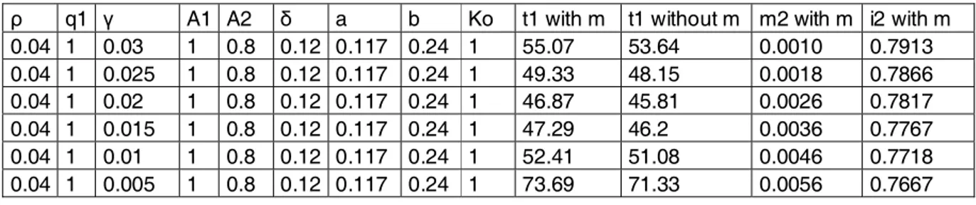
Technology Acceleration: Surprisingly, any technology acceleration parameter increase does not result with an adoption timing decrease. In smaller values of γ, an increase in the technological progress rate results in decrease in the adoption timing. Instead of waiting, the economy can reach same level or greater level of technology in a relatively shorter time with adopting the technology sooner. However, as the technological progress rate γ increases and gets closer to the discount rate, the economy delays the adoption mainly for two reasons. Firstly, as the adoption timing gets smaller, the maintenance spending increase and the consumption, thus the total welfare decreases. Secondly, the economy can reach much greater levels of technology by waiting and the cost of waiting (ρ − γ) decreases as the technology progress rate gets closer to the discount rate.

Analytically, obsolescence cost is linearly associated with respect to γ since ρln(q2

q1) = ρln(

eγt1

q1 ) = ργt1 when q1 is normalized to 1. On the other hand

both the growth advantage and additional maintenance cost include eγt1. Thus

the optimal adoption timing can be thought as the time where the difference of growth advantage than additional maintenance cost starts to exceed obsolescence cost. In small values of γ, an increase in γ causes a greater increase in the linearly associated obsolescence cost than the difference of growth advantage than maintenance cost. This causes optimal adoption timing decrease. However, in great values of γ, an increase in γ causes a greater increase in the exponentially associated difference of growth advantage than maintenance cost and this causes

optimal adoption timing increase.

Actually this means that there exists a threshold level for optimal technology adoption timing associated with the technology acceleration parameter. After the optimal timing decreases below a threshold level as a result of increasing technology acceleration, the adoption timing starts to increase with the increase in technology acceleration. The following proposition gives the sufficient condition for the adoption timing to increase in the without maintenance control framework.

Proposition 4.0.2 Assume A1 > ρ + γ. Normalize q1 = 1. Then, when the

op-timal technology adoption timing satisfies t∗

1 < ρ−γ1 , the adoption timing increases

when the technology acceleration parameter γ increases.

Proof: When we consider the optimality condition equation (3.14), this equation gives us t1 as an implicit function of γ. Doing the necessary algebraic

manipu-lations, we find that ∂t1

∂γ ≥ 0 when the condition t1 ≤

1

ρ−γ +

γ

(ρ−γ)(A1−ρ−γ+ργt1) is

met. With the given assumptions, it is sufficient for t1 to satisfy t1 ≤ _ρ−γ1 in order

to make ∂t1

∂γ ≥ 0 which means an increase in γ will yield an increase in t1.

¤

Finally, we need to analyze the relationship between maintenance and invest-ment activities. For this reason, we must consider an increase in the technology level. By algebraic manipulations one can reach the following relationship be-tween the investment in the second stage and the switched technology level:

i2(t) = A2− m2 −

ρ q2

(4.1) We know that ∂m2

∂q2 < 0 from the beginning. Together with this fact, it is easy

to see that ∂i2(t)

∂q2 > 0. Thus we can conclude that investment and maintenance

When the economy switches to a greater technology level, the older machines or the machines with older technology becomes less efficient compared to newer machines. Thus the economy increases the investment rate since when compared to the first stage, marginal benefit to marginal cost ratio for investment exceeds marginal benefit to marginal cost ratio of the maintenance activity. The economy thus increases the investment spending and decreases the maintenance spending respectively.

This relationship can be also observed in numerical analysis. m2 and i2 move

in opposite directions in all of the simulations except an increase in A2. But this

Chapter 5

CONCLUSION

In this study we have applied two stage optimal control technique to ana-lyze the effects of endogenous depreciation on optimal adoption problems under embodiment. Firstly, we solved a benchmark model without increasing frontier technology. In this case, in the optimal adoption the consumption level drops at the time of adoption because of the fall in the relative price of capital. This is obsolescence cost. Growth advantage of the technology adoption must exceed this obsolescence cost and the additional maintenance cost caused by the adop-tion for an immediate switch. Otherwise technological sclerosis occurs. For the benchmark case delaying adoption is never optimal. Another result we find is that under convex depreciation assumption, the optimal maintenance level decreases with adopting the higher technology.

Secondly, we introduced the increasing frontier technology. Although we could not derive the open form optimal adoption timing, we stated the conditions that the optimal adoption timing must satisfy and under which assumptions there exists such solutions for both exogenous and endogenous depreciation cases. We also analyzed numerically to understand the dynamics of adoption process. We find that maintenance and investment activities are gross substitutes in adoption process. When maintenance activity becomes more efficient by a change in pa-rameters, the adoption time is delayed. Another striking result is that, any tech-nology acceleration parameter increase does not result with an adoption timing decrease. In smaller values, an increase in the technological progress rate results in decrease in the adoption timing. However, as the technological progress rate increases and gets closer to the discount rate, the economy delays the adoption.

Further extensions may be done by applying multistage optimal control tech-nique to technology adoption decision. Also, instead of homogeneous capital stock assumption, heterogeneity in capital stock can be incorporated to the model. This heterogeneity can be supplied by a vintage capital model considering technology adoption decision. Lastly, instead of a constant efficiency loss in expertise, a finer learning algorithm can be incorporated to the model.

Bibliography

Ahn, S. (2003). Technology Upgrading with Learning Cost, CEI Working Paper Series, No.2003-21, Center for Economic Institutions, Hitotsubashi University. Boucekkine, R.,Martinez, B. and del Rio, F. (2005), Technological Progress And Depreciation, Working Papers. Serie AD 2005-22, Instituto Valenciano de Investigaciones Econmicas, S.A. (Ivie).

Boucekkine, R., Saglam, C. and Vallee, T. (2002). Technology adoption under embodiment : A two-stage optimal control approach, Universit catholique de Louvain, Institut de Recherches Economiques et Sociales (IRES) Discussion 2003007, Universit catholique de Louvain, Institut de Recherches Economiques et Sociales (IRES).

Boucekkine, R. and Ruiz-Tamarit, R., (2001). Capital Maintenance and Invest-ment : CompleInvest-ments or Substitutes ?, Universit catholique de Louvain, Institut de Recherches Economiques et Sociales (IRES) Discussion 2001012, Universit catholique de Louvain, Institut de Recherches Economiques et Sociales (IRES). Boucekkine, R., Martinez, B. and Saglam, C. (2001). Technology Adoption,

Capital Maintenance and the Technological Gap, Universit catholique de Louvain, Institut de Recherches Economiques et Sociales (IRES) Discussion 2001033, Universit catholique de Louvain, Institut de Recherches Economiques et Sociales (IRES).

Boucekkine, R., Martinez, B. and Saglam, C. , (2003). The Development problem under embodiment, Universit catholique de Louvain, Institut de Recherches Economiques et Sociales (IRES) Discussion 2003006, Universit catholique de Louvain, Institut de Recherches Economiques et Sociales (IRES).

Comin, D., and Hobjin, B., (2003). Cross-Country Technology Adoption: Making the Theories Face the Facts. Journal of Monetary Economics, January 2004. Greenwood, J., Hercowitz, Z. and Krusell, P. (1997), Long-run implications of

investment-specific technological change, American Economic Review, 87, 342-362.

Gylfason, T. and Zoega, G. (2001), Obsolescence, CEPR Discussion Papers 2833, C.E.P.R. Discussion Papers.

Jovanovic, B. (1997), Learning and Growth, In D. Kreps and K. Wallis (eds.), Advances in economics, Vol. 2, pp. 318-339. London: Cambridge University Press..

Khan, A. and Ravikumar, B. (2000), Costly technology adoption and capital accumulation, Working Papers 00-7, Federal Reserve Bank of Philadelphia. McGrattan, E. and Schmitz, J. (1999), Maintenance and Repair: Too Big to

Ignore, Federal Reserve Bank of Minneapolis Quarterly Review23, 2-13. Mullen, J. K., and Williams, M., (2004).Maintenance and repair expenditures:

determinants and tradeoffs with new capital goods, RePEc:eee:jebusi:v:56: y:2004:i: 6:p:483-499

Nelson, R., and Caputo, M., (1997). Price Changes, Maintenance, and the Rate of Depreciation.Review of Economics and Statistics, 79(3), 42230.

Nickell, S. (1975),A Closer Look at Replacement Investment, Journal of Economic Theory 10, 54-88.

Parente, S. (1994), Technology adoption, learning by doing, and economic growth. Journal of Economic Theory 63, 346-369.

Saglam, C. (2002) Optimal sequence of technology adoptions with finite horizon via multi-stage optimal control. Mimeo, IRES-Universite catholique de Lou-vain.

Solow, Robert M., (1956). A contribution to the theory of economic growth, Quarterly Journal of Economics, Vol.70 No.1, (February 1956): 65 - 94. Storchmann, K. (2004). On the depreciation of automobiles: an international

comparison, Transportation, 31, 371408

Tomiyama, K. and Rossana, R. (1989), Two-stage optimal control problems with an explicit switch point dependence: Optimality criteria and an example of delivery lags and investment,Journal of Economic Dynamics and Control 13, 319-337.

Appendix

Table 1: Effect of a change in technology acceleration

ρ q1 γ A1 A2 δ a b Ko t1 with m t1 without m m2 with m i2 with m

0.04 1 0.03 1 0.8 0.12 0.117 0.24 1 55.07 53.64 0.0010 0.7913 0.04 1 0.025 1 0.8 0.12 0.117 0.24 1 49.33 48.15 0.0018 0.7866 0.04 1 0.02 1 0.8 0.12 0.117 0.24 1 46.87 45.81 0.0026 0.7817 0.04 1 0.015 1 0.8 0.12 0.117 0.24 1 47.29 46.2 0.0036 0.7767 0.04 1 0.01 1 0.8 0.12 0.117 0.24 1 52.41 51.08 0.0046 0.7718 0.04 1 0.005 1 0.8 0.12 0.117 0.24 1 73.69 71.33 0.0056 0.7667

Table 2: Effect of a change in expertise loss

ρ q1 γ A1 A2 δ a b Ko t1 with m t1 without m m2 with m i2 with m

0.04 1 0.02 1 0.95 0.12 0.117 0.24 1 37.85 37.22 0.0034 0.9279 0.04 1 0.02 1 0.9 0.12 0.117 0.24 1 40.69 39.92 0.0031 0.8792 0.04 1 0.02 1 0.85 0.12 0.117 0.24 1 43.69 42.78 0.0029 0.8304 0.04 1 0.02 1 0.8 0.12 0.117 0.24 1 46.87 45.81 0.0026 0.7817 0.04 1 0.02 1 0.75 0.12 0.117 0.24 1 50.26 49.04 0.0024 0.7329 0.04 1 0.02 1 0.7 0.12 0.117 0.24 1 53.88 52.49 0.0022 0.6842

Table 3: Effect of a change in a

ρ q1 γ A1 A2 δ a b Ko t1 with m m2 with m i2 with m

0.04 1 0.02 1 0.8 0.12 0.12 0.24 1 46.89 0.0027 0.7816 0.04 1 0.02 1 0.8 0.12 0.117 0.24 1 46.87 0.0026 0.7817 0.04 1 0.02 1 0.8 0.12 0.1 0.24 1 46.84 0.0022 0.7822 0.04 1 0.02 1 0.8 0.12 0.06 0.24 1 46.76 0.0011 0.7832 0.04 1 0.02 1 0.8 0.12 0.02 0.24 1 46.70 0.0003 0.7840 0.04 1 0.02 1 0.8 0.12 0.01 0.24 1 46.68 0.0001 0.7842

Table 4: Effect of a change in b

ρ q1 γ A1 A2 δ a b Ko t1 with m m2 with m i2 with m

0.04 1 0.02 1 0.8 0.12 0.117 0.99 1 46.67 0.0000 0.7843

0.04 1 0.02 1 0.8 0.12 0.117 0.7 1 46.68 0.0000 0.7843

0.04 1 0.02 1 0.8 0.12 0.117 0.4 1 46.80 0.0013 0.7830

0.04 1 0.02 1 0.8 0.12 0.117 0.24 1 46.87 0.0026 0.7817

0.04 1 0.02 1 0.8 0.12 0.117 0.2 1 46.88 0.0028 0.7815

Table 5: Effect of a change in initial capital stock

ρ q1 γ A1 A2 δ a b Ko t1 with m t1 without m m2 with m i2 with m

0.04 1 0.02 1 0.8 0.12 0.117 0.24 0.25 46.87 45.81 0.0026 0.7817 0.04 1 0.02 1 0.8 0.12 0.117 0.24 0.5 46.87 45.81 0.0026 0.7817 0.04 1 0.02 1 0.8 0.12 0.117 0.24 1 46.87 45.81 0.0026 0.7817 0.04 1 0.02 1 0.8 0.12 0.117 0.24 2 46.87 45.81 0.0026 0.7817 0.04 1 0.02 1 0.8 0.12 0.117 0.24 4 46.87 45.81 0.0026 0.7817 0.04 1 0.02 1 0.8 0.12 0.117 0.24 8 46.87 45.81 0.0026 0.7817

Table 6: Effect of a change in discount rate

ρ q1 γ A1 A2 δ a b Ko t1 with m t1 without m m2 with m i2 with m

0.06 1 0.02 1 0.8 0.12 0.117 0.24 1 32.51 31.43 0.0039 0.7648

0.05 1 0.02 1 0.8 0.12 0.117 0.24 1 37.73 36.69 0.0034 0.7731

0.04 1 0.02 1 0.8 0.12 0.117 0.24 1 46.87 45.81 0.0026 0.7817

Figure 1: Visualization of Proposition 3.1.1

Figure 2: Visualization of Proposition 3.2.1