Analysis of multimedian problems on time dependent networks

(1)

(2)

ANALYSIS OF MULTIMEDIAN

PROBLEMS ON TIME

DEPENDENT NETWORKS

A THESIS

SUBMITTED TO THE DEPARTMENT OF INDUSTRIAL ENGINEERING

AND THE INSTITUTE OF ENGINEERING AND SCIENCE OF BILKENT UNIVERSITY

IN PARTIAL FULFILLMENT OF THE REQUIREMENTS FOR THE DEGREE OF

MASTER OF SCIENCE

By

F. Sibel Salman

July, 1994

(3)

Нс

*** ИЛ"

(4)

I certify that I have read this thesis and that in my opinion it is fully adequate, in scope and in quality, as a thesis for the degree of Master of Science.

Assoc. Prof. Barbaros Q. Tansel (Advisor)

I certify that I have read this thesis aind that in my opinion it is fully adequate, in scope and in quality, as a thesis for th ^ e g ree ja f Master of Science.

ustafa Akgiil

I certify that I have read this thesis cuid that in my opinion it is fully adequate, in scope and in quality, as a thesis for the degree of Master of Science.

AsWcT ProfT Cemal Dinçer

Approved for the Institute of Engineering and Science

Prof. Mehmet Bara Director of the Institute

(5)

ABSTRACT

ANALYSIS OF MULTIMEDIAN PROBLEMS ON TIME

DEPENDENT NETWORKS

F. Sibel Salman

M.S. in Industrial Engineering

Advisor: Assoc. Prof. Barbaros

Q .

Tansel

July, 1994

Time dependency arises in transportation and computer-communication net works due to factors such as time varying demand, traffic intensity, and road conditions. This necessitates a locational decision to be based on an analysis involving a time horizon. In this study, we analyze multi-median problems with linear demand functions on both tree and cyclic networks in a continuous time domain. The trajectory of the optimal solution is a piecewise linear concave function. We develop an algorithm that constructs the trajectory by solving 0{q) static problems, where q is the number of linear pieces in the trajectory. The properties of the optimal solution over the time horizon are also analyzed for various randomly generated problem instances.

K eyw ords: Dynamic Multimedian Problem, Parametric Analysis, Trajectory Construction.

(6)

ÖZET

ZAMANA BAĞIMLI SERİMLERDE ÇOK TESİSLİ YER

SEÇİMİ PROBLEMİNİN ANALİZİ

F. Sibel Salman

Endüstri Mühendisliği, Yüksek Lisans

Dcimşman: Doç. Dr. Barbaros Ç. Tansel

Temmuz 1994

Zamanla değişen talep, trafik yoğunluğu, yol durumu gibi faktörler ulaşım ve haberleşme serimlerini zamana bağımlı kılabilir. Bu durumda tesis yer seçimi kararının bir zaman sürecini içeren analize dayanması gerekir. Bu çalışmada, ağaç ve genel serimlerde çok tesisli yer seçimi probleminde talepler zamana bağımlı doğrusal fonksiyonlar olarak alınmıştır. Optimal çözümün izdüşümü parçalı doğrusal bir fonksiyondur. Parça sayısı q ise, 0{q) statik problem çözerek izdüşümü hesaplayan bir algoritma geliştirilip, optimal çözümün değişim özellikleri analiz edilmiştir.

Anahtar Sözcükler: Zamana Bağımlı Çok Tesisli Yer Seçimi Problemi, Parametrik Analiz, Optimal Çözümün izdüşümü.

(7)

ACKNOWLEDGMENTS

This thesis would not have been possible without the sympathetic aid given and the deep interest shown by my supervisor, Assoc. Prof. Barbaros Ç. Tansel. His invaluable instruction in the field of operations research, especially in location theory has been my constant guidance and source of inspiration. I would like to express my thanks to both members of my thesis committee. Assoc. Prof. Mustafa Akgûl and Assoc. Prof. Cemal Dinçer for their valuable comments.

Special thanks are due to other professors and fellow students, who helped me in the preparation of this thesis, especially Selçuk Avcı and Hakan Ozaktaş for providing me with their codings and Alper Atamtürk for his kind help.

I cannot fully express my gratitude to Ayşe Cankara and Giirkan Salk for their invaluble help and support.

My thanks also go to my former and current ofBcemates, Bahar Kara and Muhittin H. Demir, who supported and encouraged me throughout my studies. I would like to express my deepest thanks to my family for making it possible.

(8)

List of Figures

3.1 An example to the trajectory, z ( t ) ... 21

3.2 Alternate solutions at a b re a k p o in t... 24 3.3 Possibility la ... 26 3.4 Possibility Ib ... 27 3.5 Possibility I l a ... 28 3.6 Possibility I lb i... 29 3.7 Possibility I l b i i ... 30

3.8 Possibilities at end points ... 31

3.9 Tree structure of the example p r o b le m ... 34

3.10 Example problem, step 1 ... 35

3.11 Example problem, step 2 ... 35

3.12 Example problem, steps 3 and 4 ... 36

3.13 Example problem, trajectory... 37

3.14 Solution on the n e tw o rk ... 37

3.15 The flow tree of the alg o rith m ... 39

3.16 Points at which static problems are s o lv e d ... 45

(11)

LIST OF FIGURES vin

3.17 Length between nearest intersection p o in ts ... 46

4.1 An example p_ML(t) problem on a star n etw o rk ... 72

4.2 An example p_ML(t) problem on a general n e tw o rk ... 72

4.3 An example p_ML(t) problem on a line n e tw o rk ... 73

4.4 An example to discontinuity in individual facility movements in a p-MML(t) problem on a line n etw o rk ... 74

4.5 An example to discontinuity in individual facility movements in a p_MML(t) problem on an arbitrary tree ... 75

4.6 An example to discontinuity in individual facility movements in a p_MML(t) problem on a general netw o rk ... 75

4.7 An example to backtracking in a p_MML(t) problem on a general n e tw o rk ... 76

(12)

List of Tables

4.1 Average run times for p_MML(t) problems on tree networks . . 61 4.2 Average run times for p_MML(t) problems on general networks,

Pg 1 ... 62 4.3 Average run times for p_MML(t) problems on general networks,

pg 2 ... 63 4.4 Average run times for p_ML(t) problems on general networks . . 64 4.5 Average run times for p_ML(t) problems on tree networks . . . 65 4.6 Maodmum and most frequently observed q in p_MML(t) prob

lems on tree networks... 67 4.7 Maximum and most frequently observed q in p_MML(t) prob

lems on general networks, pg 1 ... 68 4.8 Maximum and most frequently observed q in p_MML(t) prob

lems on general networks, pg 2 ... 69 4.9 Maximum and most frequently observed q in p_ML(t) problems

on general networks... 70 4.10 Maximum and most frequently observed q in p_ML(t) problems

on tree networks ... 71

(13)

Chapter 1 Introduction

1.1 M otivation

The importance of facility location decisions can be emphasized by the fact that over 250 billion dollars is annually spent in the U.S. alone on establishing new facilities and modifying them later on. Incorrect decisions are too costly that any decision must be well justified after a thorough analysis. In accordance with these considerations, a lot of research has focused on facility location and theories have been developed for various facility location problems for over 50 years. An overview of research on facility location can be found in Î7İ and [51],[52].

Traditional approaches have considered the location problem as a static one and assumed that the location determined according to present conditions would sustain its superiority throughout the lifetime of the facility. However, tis an examination of changes in number, location, size and product variety of plants of a sample of 64 small and medium sized multiplant enterprises over 6 years by Healey [34] shows, facilities are subject to various changes among which locational changes have high frequency. Facilities operate in a dy namic environment influenced by technological innovations, cycles of economy, changes in tastes and environmental factors. Demand patterns not only change in the long run due to factors like population shifts, changing income levels, development of competing products, failing to keep customer satisfaction, but also in the short run due to seasonality and promotion campaigns. In addition

(14)

CHAPTER 1. INTRODUCTION

to demand changes, costs relevant to the location decision like transportation costs, labor cost, taxes, rental costs, are subject to changes that can usually be successfully predicted by forecasting methods. Thus, the dynamics of the problem have to be incorporated into a location decision to prevent a myopic decision that could cause the locations to be unattractive by time. As different locations become optimal at different times, the initial locations may fall to be suboptimal by time. Then, an analysis involving an appropriate time horizon, such as the forecasted life-time of the facility, is required. The decision of ei ther relocating the facilities throughout the time horizon, following the path of the optimal locations, or choosing permanent locations at the beginning of the time horizon which will be close to the optimal locations should be made. This decision depends on the tradeoffs between the costs of relocating the facilities, including non-monetary terms like the resistance of the organizations, and the savings from operating costs as a result of the relocations. If costs appear to overweigh, permanent locations would be chosen and it is worthwhile to try to turn the locations into favorable ones by promotional activities. In some cases, relocations can easily be justified, as in the case of mobile or portable service facilities where the optimal locations could be followed. Thus, knowing exactly what locations will be best in what time intervals is an asset in both situations.

Let us consider mobile facilities serving demand centers scattered in a re gion over a time horizon, for example, a military base in a war situation in coordination with quairters that might change their locations frequently due to strategic reasons or a tourism information booth that serves demand which shows seasonal variations. It is reasonable then to determine how optimal so lutions change in response to the dynamic factors and to follow the optimal path.

Another situation in which relocating the facility over time may be preferred and easily accomplished is that of determining which machines will perform special tasks like control of information routing, storage etc., depending on the changing traffic intensity on a computer and communication network. In this case, relocations are ignorably incostly and extremely manageable.

Even though relocating the facilities could be too costly and problematic, for a decision that considers an appropriate time horizon, knowledge about the

(15)

optimal locations of the facilities throughout the planning horizon would be helpful. For example, consider warehouses from which non-durable goods are distributed to retail stores in a city. The ”rush-hour” behavior of traffic that causes travel times to vary within a day can be fairly well predicted. Obviously, relocating warehouses within a day is out of consideration. However, knowing the optimal trajectory of the locations throughout the day may be useful in choosing a location that would be better off for normal traffic intensity and would not be undesired for rush-hour periods.

1.2 D ynam ic Location Problem s in th e Literature

Against static facility location problems which depict a single-period or static situation, dynamic facility location models which reflect a multiperiod or time dependent situation were posed about a quarter century ago.

Dynamic facility location problems raise the question of when to establish and if necessary to replace a productive capacity due to changing conditions in addition to the classical questions of where and what size.

A dynamic location problem was first studied by Ballou [1] who considered multiperiod warehouse location problem with capacity constraints (1968). He gave an approximate solution by dynamic programming and later Sweeney and Tatham [48] solved the problem to optimality by dynamic programming with an extended state space. Wesolowsky [53] examined multiperiod single facility location-relocation problem. Relocation of the facility is permitted only at the beginning of the periods with the assumption that amount of demand, number of demand points, distribution and relocation costs are constant within a period but may change between periods. Relocation cost is assumed to be indepen dent of the location of the facility before and after relocation, which is actually unrealistic. Wesolowsky gave an incomplete dynamic programming algorithm that finds the optimal locations in each of the r periods by solving O(r^) static problems. Later, Wesolowsky and Truscott [54] extended this model to a multi facility location-allocation problem and presented mixed integer programming as well as dynamic programming solutions.

(16)

Afterwards, there appeared numerous studies in the literature about dis crete time location models with a multiperiod situation where demand varies between time periods, usually with an increasing trend. Thus, capacity ex pansion was also considered in addition to location and relocation aspects. Such problems are discussed in detail in Chapter 4, "Multiperiod Capacitated Location Models”, of Discrete Location Theory [42]. A general multiperiod capacitated location model whose solution requires the minimization of a non linear, concave function over a polyhedron, is presented by Jacobsen in this chapter. The solution methods are gradient search algorithms and dynamic programming.

Erlenkotter [25] studied uncapacitated dynamic location problems and for mulated problems in the private, public and quasi-public sectors, where de mands are influenced by prices at various locations so that pricing and loca tion decisions are determined simultaneously. He showed that these problems may be transformed to the fixed-demand location model of Efroymson and Ray which may be solved by available methods. Later, Van Roy and Erlenkotter [45] gave a dynamic uncapacitated facility location model that minimizes total discounted costs for meeting demand over time with the flexibility of opening new facilities and closing existing ones by time. A branch and bound procedure which incorporates a dual ascent method is presented and is claimed to be supe rior to previous methods. Erlenkotter also gave a continuous time formulation in [24] and suggested a discrete-time approximation heuristic solution.

One recent discrete-time model is Dutta and Lim’s [20] multiperiod capacity planning model for computer and communication networks. The model allows traffic among existing nodes to increase, new nodes to be added to the network and its topology to change over time. The model is formulated as an IP and a Lagrangian relaxation based solution method is proposed. Shulman [47] also gave an algorithm based on Lagrangian relaxation technique for solving dynamic capacitated plant location problems with discrete expansion sizes.

Chand [11] examined dynamic location problem from a different aspect and addressed the problem of finding decision and forecast horizons for a sin gle facility dynamic location problem. He defines a decision horizon to be the number of periods for which decisions have to be made now. A forecast horizon is defined to be the number of periods of forecast data required to ascertain

(17)

optimality of the initial decisions over the decision horizon and gives a for ward procedure to find an optimal initial decision. Bastian and Volkmer [2] claimed that Chand’s algorithm is not ’’perfect” in the sense that it does not determine an optimal initial decision using only data for the minimum forecast horizon. They presented a more general relocation model and a perfect forward algorithm to solve it.

Heuristic methods for multiperiod location problems are discussed in Ja cobsen [35] and Erlenkotter [27] compares the performance of 7 approximate methods for locating new capacity over time to minimize the total discounted costs of meeting growing demand at several locations on two real-world prob lems.

More information on discrete time dynamic location problems can be found in the bibliography prepared by Erlenkotter [23] and a survey paper by Luss [40]. A recent study by Hakimi, Labbe and Schmeichel [31] not only reviews dynamic location problems but also discusses some interesting modeling as pects.

Dynamic facility location models in a continuous time domain are researched by Orda and Rom [43], Drezner and Wesolowsky [19], Campbell [10] and Tansel 180].

Orda and Rom [43] address a single-facility dynamic network location prob lem within the context of computer and communication networks. As a mod eling convenience, the location space is restricted to the nodes of the network and the edge lengths are defined to be positive functions of time. The objective function to be minimized consists of the cost of locating the facility at certain nodes and the cost of switching the facility, if any occurs, throughout the time horizon. General costs are used in the model. The location cost in a time in terval in which the facility remains fixed in its location is the integration of the instantaneous cost of having the facility at its location over that time interval, where instantcineous cost is defined by any performance measure. Switching cost depends on the locations before and after the switch as well as the time in which it takes place. The cost is assumed to be non-decreasing with the duration of switch and goes to infinity in the limiting case of zero duration. It is also assumed to be a continuous or piecewise continuous function of time.

(18)

Discrete time version of the model is solved by a shortest path algorithm on a network that has as many levels of the original nodes as the number of periods, k. Each node in a level is connected to each node in the next level with appropriate costs determined by location and switching cost functions at this period. A source node with no cost of edges is connected to each node in level k-1 with only appropriate location costs.

For the continuous time model they give an algorithm which first computes the cost of the optimal locations throughout the planning horizon and then calculates the locations. The algorithm is like a limiting shortest path algo rithm on a network with levels for each time period. The algorithm stops after a finite number of iterations when there is no change in the cost functions between iterations. No time bound is given for this exact algorithm.

Drezner and Wesolowsky [19] also investigate facility location when demand varies with continuous time in a predictable way. They study single facility minisum problem on a planar location space with weights being nonnegative time functions. The location of the facility can be changed during the time horizon but each relocation incurs a fixed cost. The decision variables are time points at which the facility changes location, i.e. breakpoints and the location of the facility in each time interval between breakpoints. For the special case of rectilinecir distances, linear weights and the restriction that only one breakpoint is allowed, the problem is solved using the property that the static problem decomposes into two one-dimensional problems, each with a solution on a demand point, as well as the monotonicity of the optimal location due to linear weights. The algorithm goes as follows. First, the solution for time zero is found and the smallest breakpoint b' among the breakpoints of switching to a pair of adjacent coordinates is identified. Once the locations before and after time point b' are known, F{b), the objective value with these locations and a breakpoint at 6, where b is taken as a parameter, is computed. Beginning with the time bo, which minimizes F{b) in the interval [0, 6'], the process is repeated until the next smallest breakpoint is beyond the time horizon or does not exist. Then, among bo's, calculated during the process, the one with minimum F{bo) is the optimal breakpoint and F{bo) is the optimal objective value.

When more than one breakpoint is allowed, they propose a heuristic based on a univariate search with breakpoints. They initially divide the time horizon

(19)

into k segments. Repeatedly, one-break point problem is solved by keeping all but one breakpoint fixed. The procedure stops when no significant changes in breakpoints occur.

The authors also give a minimax version of the weight parametric model. Two algorithms which find the solution to the problem with k relocations is given. Then, a search on k is suggested. The algorithms can be applied to a weight parametric p_center problem on a network with the assumption that a fixed relocation cost is incurred at breakpoints whatever the number of centers that are to be relocated.

Another interesting relocation model in a continuous time domain is given by Campbell [10]. The model incorporates locating transportation terminals in a service region with an expanding demand. Shipments are sent from ori gins to destinations scattered over this region via one or more terminals since shipments between terminals are less costly. The tradeoffs between savings in transportation costs and terminal relocation and establishment costs determine when and where terminals should be added and relocated.

Campbell analyzes the performance of three strategies. One is relocating terminals as many times as required by the minimization of only transporta tion and terminal establishment costs. The other two are allowing no relo cations and relocation of only one existing terminal when a new terminal is added. Comparison of the strategies in terms of difference from a lower bound suggests that optimal solutions can be reached by limiting the number of re locations when relocation costs are low. With high relocation costs, making no relocations can be preferred, however the solution may not be very close to optimal.

Tansel [50] considers the time dependent version of the single/multi me dian problem for which weights or distances are functions of time. Various node optimality results are given, a penalty minimization problem is defined and solved. The multi-relocation problem is analyzed by transforming the problem into a rectilinear path problem on time coordinates. By an intermedi ate value optimality theorem, finitely many points on the plane through which the optimal path must go are identified. Then, the problem becomes that of finding a shortest path on a network whose nodes correspond to the identified points.

(20)

Another perspective in the analysis of dynamic facility location problems is parametric analysis which involves determining the optimal locations for cer tain values of a parameter inherent in the model. While Brandeau and Chiu [6] analyzed single-median problems with an Lp-norm based objective function with parameterization on p, Erkut and Öncü [21] analyzed single obnoxious facility location problem with parametric weights. Erkut and Tansel [22] ad dressed and analyzed time dependent single-median problems with parametric weights or distances, where the parameter is time. Brandeau and Chiu [9] summarized recent results on parametric analysis of a single facility location for various location problems.

Brandeau and Chiu [6] analyze the optimal location of a single facility on a tree network with the objective of minimizing the sum of weighted ip_norm distances from each node to the facility, as the parameter p changes in the interval [l,oo). As p increases, the cost becomes more sensitive to distance. Thus, parameterization is on customer disutility for travel. For p = 1, we have the median problem and for p = oo, the problem becomes unweighted center problem. For fixed p, optimality conditions are given using directional deriva tives and the trajectory of the optimal location is constructed by a method that hinges on the convexity of the objective function. It is shown that the op timal trajectory is continuous and need not be monotonie between the median and center locations. The method of finding the trajectory fails for a cyclic network since the objective function need not be convex anymore. It is also shown that nonconvexity can lead to a discontinuous, disconnected trajectory. The conditions for having a continuous trajectory of the optimal location to single facility parametric location problems are given in a separate note by the authors [5].

Erkut and Öncü [21] introduce a parametric version of the weighted l_maximin i

problem in a convex polygon, where parameterization on weights (tw*, 1 < ç < oo) creates a range of problems with different importance of weights, from ordinary weighted one to the unweighted version. Optimal trajectory is constructed for two example problems and it is concluded that the trajectory may be discontin uous and radically different optimal locations can be found for different values of the parameter.

(21)

with parametric node weights for the cases of weights being linear and nonlin ear functions of time. A "connectedness” theorem stating that the trajectory of optimal solutions over the time horizon is connected and is in the form of a subtree, is given for the general case of nonlinear weights. For the problem with linear weights, this subtree reduces to a path between the optimal locations to the problems at the end points of the time horizon. Using the half-sum prop erty, the trajectory of the optimal solution is constructed in 0 (n) time, n being the number of nodes in the tree. The connectedness result also facilitates the construction of the optimal trajectory of the problem with nonlinear weights. However, the efficiency of the construction method depends on the effort re quired to solve nonlinear equations and the total number of breakpoints in the trajectory.

Brandeau and Chiu [9] summarize recent results on parametric analysis of the optimal location of a single facility on a network or a planar region. The parametric problems addressed are cent-dian problem introduced by Halpern [32] [33] whose objective function is a linear combination of center and median objectives, problems that use an Lp_norm based cost function introduced by Shier and Bearing [46], stochastic location problems with parameterization on the customer call rate [3], [4], [8], [15], [16] and dynamic facility location problems where demands or distances may change over time [19], [21].

With the assumption of unique optimal solution at a fixed value of the parameter and continuity of the trajectory of the optimal location, a method for determining the trajectory is presented by the authors. For the median problem with demands being time functions uniqueness does not hold, thus the method presented is not applicable. Although parametric 1 .median problem is analyzed by Erkut and Tansel [22] as explained above, there is no study in the literature for the parametric multimedian problem.

CHAPTER 1. INTRODUCTION 9

1.3 Scope o f th e T hesis

In this study we focus on parametric multimedian problems. We examine pjnedian and pjnedian with mutual communication problems with weights being linear functions of time both on tree and cyclic networks. We assume

(22)

CHAPTER 1. INTRODUCTION ₁₀

that changes in demand or costs over time are predictable. Since linear re gression is frequently used for short and medium term forecasts, it may be acceptable to represent future weights as linear functions. For long term fore casts, nonlinear demands can be approximated by piecewise linear functions. Our analysis for the linear case can easily be extended to the piecewise linear case by partitioning the time horizon into intervals each with linear demands.

We construct the trajectory of the optimal solution over the time horizon [0,u), by an algorithm that requires the solution of 0{q) static pjnedian prob lems, where q is the number of linear pieces in the trajectory. In this study, the term ” static problem”, will be taken to mean the relevant problem for a fixed value of the parameter time. When we use the term ” trajectori/\ we mean the time path of the objective value of the optimal solution to the problem at a time point, over the time horizon. By "time horizon”, we mean the continuous time interval for which the optimal locations of the facility are intended to be determined. The term ” breakpoints” will be used to mean time points at which the optimal locations change by at least one location in the trajectory.

We have implemented the algorithm that constructs the optimal trajectory and analyzed the behavior of some randomly generated problem instances. Trajectories of p_median and pjnedian with mutual communication problems were analyzed for special type trees like line, star eis well as arbitrary trees and cyclic networks with various edge density factors. In the analysis, the emphasis is on tree networks since this study originated to analyze the problems on tree networks and then extended to general networks as well.

The general parametric multimedian problem is introduced in Chapter 2. Chapter 3 examines the case with linear weights. The algorithm to construct the trajectory is also presented in this chapter. Chapter 4 summarizes the design of experiments and results from their analysis. Finally, we conclude and give future research directions in Chapter 5.

(23)

Chapter 2 Multimedian Problems on Time

Dependent Networks

With the goal of reaching optimal locational decisions, many prescriptive lo cation models have been developed for the last three decades. The literature is huge and rapidly growing. Yet, among numerous formulations, pjnedian, p_center, uncapacitated facility location and quadratic assignment problems are considered to be basic model types. Among these problems, we concentrate on pjnedian problem and present its time dependent version in this chapter.

2.1 T he Clcissical p_M edian P roblem

For a given value of p, the p.Median Problem is to find locations of p facilities to be established and to supply each client from a subset of facilities such that the demands of clients cire fully met and the costs incurred are minimized. Facilities are uncapacitated in the sense that they can serve any number of clients and supply any amount of demand. Nothing is gained from serving a client from more than a single facility, so the problem hcis the Single-Assignment Property ( Dominance Property ). Other assumptions are that demand is fixed and independent of server location, a single client is served by a single trip and all facilities are identical in the sense that they are operated by one firm or are non-competing. With these assumptions finding only the locations of facilities suffices. Each client is served by the least costly facility.

(24)

CHAPTER 2. Tí m e d e p e n d e n t m u l t i m e d i a n p r o b l e m s ₁₂

A general formulation of the p_median problem by a bipartite network is as follows.

Let I denote the set of clients, I = {1, . . . ,m}

and J denote the set of potential facility sites, J = {1,... ,n}

The bipartite network Nb = (V,E) = ( I U J,E) has the sets I and J as its set of nodes and E as the set of edges. Each arc connects a node in I with a node in J.

Let c be a real valued cost vector associated with the edges. If facility j cannot supply client i, c,j = oo. Given the data instance m ,n,p and c = {c,j}, the p_median problem is.

p_MP : min (

QÇJ.IQNpV

The pjnedian problem was first formalized by Weber (1909). His model was a minisum location problem on a plane. The term ” pлnedian” was intro duced by Hakimi [30] within the context of network location. Hakimi assumed that the cost of serving a client from a facility is proportional to deterministic distance between them. His ponedian problem is as follows.

Suppose we are given a network N = (V,E) with node set V = {ui,...,Un} and edge set E. Each edge e in E has a positive length /(e). We denote by L the set of all points of the network. L is our location space. A point x in L is either a node or a point in some edge e = [vp, u,j such that it divides the edge into two subedges [up,x] and [x,u,j satisfying /( [vp,Vq] ) = /( [up,x] ) -1- /( [x,u,| ). The length function / induces a distance d on L which assigns a real value d(x, y) to every pair of points x,y in L. Here, d{x,y) is the length of a shortest path connecting X and y. Note that d defines a distance metric so that it satisfies the following properties for all x ,y £ L.

1) Nonnegativity : d{x,y) > 0 , d(x,y) = 0 iff x = у 2) Symmetry : d(x, y) = d(y, x)

(25)

CHAPTER 2. TIME DEPENDENT MULTIMEDIAN PROBLEMS 13

Let Wi be a nonnegative weight cissociated with node u,·, i.e. Wi represents the demand at node u,. Then, the p_median problem is:

P-M : n n n ^ E i^ i ti^, m in{i/(xj,n,) : x j G ,

where X = { i i , 3:25 · · · » } ¡s a set of p points in L , where facilities are to be established, i.e. a p_median. Actually, Hakimi differentiated between abso lute pjnedians and vertex p_medians. He called the set X an absolute p-tnedian when the points are allowed to be any point in L and a vertex p.median when the points are chosen among vertices. Then, he showed by his ” Node Opti mality Theorem ” that there exists an absolute p_median whose elements are all vertices. Therefore the distinction is unimportant. We refer to the above problem as the classical p_median problem and to its optimal solution as a p_median.

The p-median problem was discussed in detail by Kariv and Hakimi [36] who showed that the problem of finding a p_median of a general network is NPJiard. However, they gave a polynomial time algorithm to find the P-median when the network is a tree. Generalizations of the p_median prob lem are discussed in detail in a survey paper by Tansel et. al. [51] and in the 2”*^ Chapter of Discrete Location Theory [42]. At this point we suffice with introducing the problem and delay the discussion of the solution methods until Chapter 4.

2.2 T he p_M edian w ith M utual C om m unication P rob

lem

The p.Median with Mutual Communication Problem is to find the location of p new facilities which are in interaction with each other and the existing n facilities, to minimize the sum of the costs of interaction. The costs of interaction are represented as weighted distances between pairs of new and existing facilities, and pairs of new facilities. Facilities are distinguishable. While existing facilities are distinctly located, new facilities may well be located at the same site. An existing facility can be in interaction with more than one new facility, therefore the single-assignment property is not applicable in this

(26)

scenario.

The problem was first posed with a planar location space by Francis [28]. The solution methods under different distance metrics are discussed in Chapter 5 ’’Multifacility Location Problems” of Facility Layout and Location by Francis, McGinnis and White [29]. The problem on a network is defined by Bearing, Francis and Lowe [17] in the presence of distance constraints. The authors show that the problem is a convex optimization problem for all data choices if and only if the network is a tree. For the case of a general network, there exists an optimal solution on the vertices of the network. The problem on a network is formulated as follows:

• Suppose our location space L is a network N = (V,E), where the set of ver tices V represents the locations of the existing facilities. The function d{.,.), as defined above for the classical p_median problem, denotes the distance between two points on the network which is induced by the edge lengths. We represent nonnegative weight cissociated with the interaction between the existing facility at node u,· and the new facility at location xj by Wji, and that of between the new facilities at locations Xj and Xk by Vjk- The problem is:

p_MM : imn Eî=ı Wjid{xj, u.) + E L j+ i Vjkd{xj, i*) j

Here, X = { Xi,X2, . ■ ■ ,Xp ) denotes p points in L , where new facilities are to be located. X is a vector since the new facilities are distinguishable. It is possible, for example, to have x,· = Xj for i j so that facilities i and j are located at the same point.

The problem on a general network is shown to be NPJiard by Kolen [39], while polynomial time algorithms have been given by Picard and Ratliff [44], and Kolen [38] on a tree network. Furthermore, Tamir [49] has shown that the problem is NP_hard even on a tree, if we restrict the location of each new facility to a proper subset of vertices. Although efficient algorithms have been presented for the problem on a tree network, there has not been any efforts on solving the problem on a general network, with the exception of Chhajed and Lowe [13] who gave a polynomial time algorithm when the communication between new facilities can be represented by a series-parallel graph. The so lution methods will be discussed in Chapter 4 as the experimental studies are

(27)

CHAPTER 2. TIME DEPENDENT MULTIMEDIA N PROBLEMS 15

presented.

2.3 T im e D ependen t p_M edian Problem s

Time dependency can arise either by weights or edge lengths being functions of time, or both. \V^ first define a general time dependent p_median problem with both weights and edge lengths being functions of time. Then, we focus on the weight parametric case.

The time dependent p_median problem is to find the locations of p facilities to be established so that the costs incurred from supplying changing demands of all clients with changing distances to each other over the time horizon [0,u] is minimized at all time points in [0,u].

Suppose that node weights ( Wi{t) ), i.e. client demands and edge lengths ( /(e,t) ) are nonnegative continuous functions of time such that the ratio of a subedge length to the entire edge length is constant for t € [0,u]. The length function /(.,t) induces a time dependent distance function d{x,y,t) which as signs a real value to every pair of points x,t/ in L at a time point t. In accor dance with the static case, d{x,y,t) is the length of a shortest path between

X and y when edge and subedge lengths are fixed at time t. The function d{., .,t) satisfies nonnegativity, symmetry and triangle inequality properties of a distance function for each fixed t. Thus, d (.,.,t) is a well defined distance function. For X = { xi,X2, ... ,Xp }, let f { X , t ) be the cost function defined as.

f{x,t) = wi{t)min{d{xj,vi,t) ·. x, e x }

With these definitions, the time dependent problem at a time point t is , p_M(t) : z(t) = rn in /(X ,t)

If we denote the set of pjnedians that correspond to the optimal objective value z(t) at time point t by Xp(t), then the time dependent pjnedian problem is to find Xopty the set of all optimal solutions throughout the time horizon [0,u] , which is defined as

(28)

^opt = { Np(t), t G (0,u| }

Here, z(t) , Vt 6 [0,u] is the trajectory of the optimal objective value. Tansel [50] has shown that node optimality holds for the time dependent case. The problem can then be restated as

P-M(t) z(t) = m m^/(X’',i)

where X'' denotes the r-th choice of p nodes and q is the number of all possible choices of p nodes. Construction of z(t) for t € [0,uj as the pointwise minimum of q functions identifies the subset of Xopt with elements that consist of vertices only, i.e. = { Xp(t) H V, t G [0,u] }

We will be focusing on the weight parametric case from now on, with the motivation of modeling situations in which demands are time varying in a predictable way. The two problems that we examine are Weight Parametric P-Median Problem and Weight Parametric p.Median with Mutual Communi

cation Problem.

The weight parametric p_median problem is the only-weight parametric version of the classical p_median problem and represents situations in which demand varies predictably by time. The formulation of the problem is as follows.

f { X, t ) - E ”=i w^.(Omin{d(a:j,Ui) : Xj G X } p_MP(t) : z(t) = rm n /(X ,i)

Using the node optimality property, the problem can be restated as. p_MP(t) : z(t) = min f { X \ t ) = u;,(i)min{d(a:J, v,·) : xJ G A’’’}

Then, the problem is to find the minimum of q functions where, q = . The definitions of A'p(t), Xopt^ Xv and z(t) are still valid.

Weight parametric p_median with mutual communication problem models the cases in which there is a time varying traffic among the new facilities in addition to the time varying traffic among new and existing facilities. If we

(29)

denote the nonnegative continuous weight between new facility j and existing facility i by Wji(t) and that of between new facilities j and k by Ujjt(t), then the problem is :

f i x , t) = Z U Wjiii)d{xj, Vi) + E U n = i + i vjkit)d{xj, Xk)

p.MMP(t) z(t) = min f { X, t )

In this problem, we denote the set of optimal location vectors at time t by Xp(t). Xopt is the set of all optimal vector solutions throughout [0,u]. If we restate the problem using node optimality property, then the formulation will be,

f ( X ’ , t)

=

T . U où

+

ELi+i

p_MMP(t) : z(t) = ^min f { X ’’,t)

Then, z(t) is the minimum of q functions, where q = n^ and X^, is the subset of Xopt that contains all elements that are vectors of p vertices.

(30)

Chapter 3 Medians with Linear Weights :

Trajectory Construction

In this chapter we focus on pjnedian problems with linear weights. As men tioned in the Introduction Chapter, short and medium range forecasts usually show a linear trend. Furthermore, long range forecasts can adequately be ap proximated by piecewise linear functions. Thus, solving the linear weights case could facilitate locational decisions in more general time dependent settings.

Within the frame of definitions made in the previous chapter, we define the two problems that we will be analyzing in this chapter, p-median problem with linear weights and p.median with mutual communication problem with linear weights. Development of an eflBcient divide_and_conquer type algorithm to construct the trajectory is presented step by step.

3.1 p_M edian P rob lem s w ith Linear W eights

The formulations of the weight parametric p_median problems were presented in the previous chapter. We obtain pjnedian problems with linear weights by inserting linear weights into these formulations.

For the p_median problem with linear weights ( p_ML(t) ), we take weights as linear functions of the form

(31)

CHAPTER 3. MEDIANS WITH LINEAR WEIGHTS 19

w,(t) = a,· + 6,· * t , Vu,· € V and t 6 [0,u] ,

where a,’s and ¿¿’s are given constants which specify a problem instance together with n, p and the network structure. We assume a, > 0 and a ,+ 6,u> 0, Vi. It follows then, for X = {xi,X2> · · · ? ^p] Q L, we have

f { X , t ) = Er=i(«i + 6i0niin{if(ij,t;,): Xj e X } p_ML(t) : rmn f { X, t ) , tG[0,u].

Since we know that there exists a choice of p vertices which minimizes f { X , t ) at a time point t, we can restrict our solution space to all possible choices of p vertices. The set of all choices of p vertices among n vertices is finite with cardinality q = Suppose that all possible choices are indexed arbitrarily from 1 to q. We denote the set of these indices by Q. With X ’’ denoting the r-th choice of node restricted p_medians, we have

f ( X ’^jt) = Ar + Br * t, where Ar = U=iC^iDiX%Vi)

Br = U=ibiD{X%Vi)

with, D {X ’’,Vi) = ^min d{Xj,Vi)

For the pjnedian with mutual communication problem with linear weights ( p_MML(t) ), we take weights between pairs of new and existing facilities as linear functions of the form

u;j,(t) = Uji + bji * t , for {j,i) € h

with h Q { {j,i) : 1 < j < p , 1 < i < n } and weights between pairs of new facilities as Vjfc(t) = ajk + ^jk * t , for {j, k) G h

with /2 ^ { (i, k) : l < j < k < p } .

In this case, the problem data is specified by the constants Oj,·, bji, {j, i) 6 h and ajk, Pjki U,k) € / 2. Assume Oj,· > 0, aj, + 6j,u> 0, max{aj,-,aj, + 6j,u} > 0

(32)

CHAPTER 3. MEDIANS WITH LINEAR WEIGHTS ₂₀

v (i, 0 6 /i and ajk > 0, Ojk + 0, max{ajfc, ajk + Pjku} > 0 V{;, k) e h

-For X = ( i i , X2> · · ·»^p) € X”*, we have

f { X , t ) =

X)

{oji + bjit)d{xj,Vi) + i^jk + 0jkt)d{xj,Xk)

(j.i)eh U<k)€h

There exists a solution vector on vertices so that we can restrict the solution space to all vectors of size p whose elements are vertices. There are q = n’’’ such vectors. Suppose that all such vectors are indexed arbitrarily from 1 to q. We denote the set of these indices by Q. With X ’^ denoting the r-th vector, we have

f { X \ t ) = Ar + B r * t

pJ^L (t) : min f { X, t ) , t6[0,u], where

^ ( j , k ) € l 2 ^ J k d ( X j , X k )

=

H{j,i)eh

d"

H(j,k)eh 0ikd{x^,Xk)·

Then, multimedian network location problems with linear weights can be represented as

PL(t) : z(t) = min / ( X ’’,i) = Ar + Br * t. T&Q

For simplicity of notation, we define

Fr{i) = / U ^ 0 · Thus, z(t) = min F,(t).

l< r< g

With z(t) being the lower envelope (pointwise minimum) of q linear func tions over the interval [0,u], we have the following lemma.

L em m a 1 : z(t) is piecewise linear concave function of t with at most q pieces.

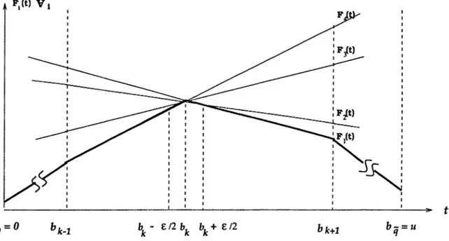
Let q be the number of pieces of z(t) and Q be the set of i 6 Q for which i^(t) is a nondegenerate piece of z(t) in [0,u]. Clearly, | Q | = 9 and q < q. Let B = {¿1, 62, · · · 5 bg-i] be the set of breakpoints of z(t) and B' be the extended set which is the union of set B, breakpoints, and the end points of the interval

(33)

[0,u]; that is,

B' = {6o , w i t h ¿>0 = 0 and bg =u. We assume that the indexing is done in such a way that bo < bi < 62 < ... < < bg.

bj=u (q = 3) Figure 3.1. An example to the trajectory, z(t)

In general, the lower envelope of q linear functions can easily be constructed in 0{q^) time. It may also be possible to do the same task with better time complexity, such as 0{qlogq). This requires knowing the two parameters of the linear functions, the intercepts and the slopes. In our case, the parameters are /4,·, Bi, Vf G Q. Since q = or nP, the computation of all A,, B( and the construction of the lower envelope z(t) via known methods takes at least

log (p)) or 0 (nP lognP) time.

We propose, however, a much more efficient method that avoids a pri ori computation of the parameters A,, Bi which are exponential in number. We construct the lower envelope by solving 0{q) static problems and compute only 0(q) of the parameters A,·, Bi on a need basis during the construction pro cess. If the static problem can be solved in 0{g{n,p)) time, then the proposed method constructs the trajectory of z(t) in 0{qg(n,p)) time. It is evident from our computational studies presented in Chapter 4, that q is typically much

(34)

much smaller than q for many instances, (e.g. among the 1350 randomly gen erated p_MML(t) problems, maximum q turned out to be 15 for the problem with n = 60 and p = 30, where q = 60^° = 2.21e+53.) Therefore, trajectory can be constructed in reasonable time for problems of large sizes, even though q is extremely large, (e.g. 10 minutes for p_MML(t) problems with n = 100 and p = 95 and 1 hour for p_ML(t) problems with the same values of n,p on tree networks.)

At this point two questions arise. One is, whether q ever equals q or there is a bound on q which is significantly smaller than q which also explains the immense gap between q and q in our experimental studies. We present two bounds on q after discussing our trajectory construction algorithm. However, there is still a huge gap between these bounds and realizable values of q in practice, the reasons of which remain to be explored. The other question is, what the least order of constructing the trajectory could be. To explore the answer to the second question, let us define the sets, Z, Zb, and S as follows.

Z = { {t,z{i)) : t e [0,u] } Zb = { (6.·, : bi 6 B' }and

5 ^ { { t, X{ t) ) : f { X { t ) ,t ) = z(i), i G [ 0,u ]}.

In our context, what we mean by constructing trajectory is finding the sets Z and S. Clearly, it suffices to know Zb to generate Z. Observe that finding each z(6,·) requires solving a static problem, since z(6,·) is defined as

z(6,·) = m in/(X , 6,·), for 0 < i < q.

Hence, construction of Zb requires solving 9 -f 1 static problems. Knowing

the solutions to these static problems, i.e. X (6,)’s, is not sufficient to construct the set S since a solution X{bi) may not be optimal at any time point different than 6,. To find a solution that is optimal between two breakpoints 6,_i and bi, a static problem solution is required at a time point t € 6,·). Thus, the least number of static problems to be solved to construct the trajectory is 2q A I- The method we propose in this thesis constructs the trajectory by solving at most 4g-2 ( 0(q) ) static problems. Therefore, we may conclude that our construction algorithm is a best order algorithm unless there exists a more efficient method of identifying optimal solutions at a time point than solving a static problem.

(35)

3.2 Trajectory C on struction

We start this section by developing some preliminary information that leads to an efficient algorithm to construct the trajectory.

3.2.1 Prelim inaries

We could construct the trajectory by solving 2^+1 static problems as explained above, if we knew the set of breakpoints, B. However, the set B is a priori unknown. A breakpoint is identified as the intersection point of two adjacent linear pieces of z(t), i.e. the intersection point of Fi{t) and Fj{t), for some i , j 6 Q. The intersection point of the functions Fi{t) and Fj(t) can be identified

^ = b' ^ whenever 5,· ^ Bj. Let T = { t : t E (0,u) and 3 i , j G Q

such that Bi ^ Bj and t = }· With this definition, T is the set of time points in (0,u) at which two ( or more ) functions intersect. We call T the set of intersection points. T has at most q{q — l)/2 elements. Observe that each breakpoint is supplied from T; that is, B Q T .

Our trajectory construction algorithm solves static problems at points which are those elements of T that are candidates to be breakpoints. Even though T ha5 0{q^) elements, the algorithm correctly selects 0(q) elements as candidates thereby eliminating a large number of intersection points from candidacy.

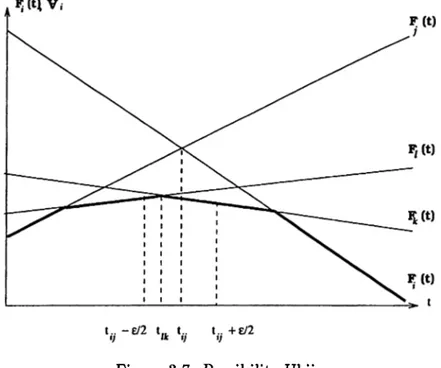
At an intersection point, more than two linear functions may intersect. If the objective value induced by intersecting functions happens to be optimal, then this point is a breakpoint. We need to find the functions that are optimal to the left and right of that breakpoint to correctly identify the solutions in [0,u]—.6 . Figure 3.2 depicts the situation.

(36)

Figure 3.2. Alternate solutions at a breakpoint

In Figure 3.2, among all alternate solutions at t = bk, we want the one that remains to be optimal at t = 6^. + e/2 for t > 6jt and at t = 6* — e/2 for t < 6jt, where e is a small positive real number. We should use such an e that there should not be any breakpoints in the intervals [6jt — e /2, fejt) and {bk,bk + e / 2].

Let £ = min (6,· — 6,_i) and £' = min (t' — t). Thus, £ and £'

specify, respectively, the minimum distance between any two distinct members of B and T. Note that B C T implies 0 < £' < £ <u. Since the breakpoints and intersection points are computed only when needed, the sets B and T are not available at the beginning. Hence, £ and £' are not a priori computable. However, it is possible to calculate a lower bound on £ and £' in terms of the problem data. The computation of such a lower bound will be given at the end of this chapter.

L em m a 2 : Let L B be a lower bound such that 0 < LB < £ ' < £ . If we choose e from (0,LB),

i) there can be at most one breakpoint, i.e. an element of B, in a time interval of length e.

ii) there can be at most one intersection point, i.e. an element of T, in a time interval of length e.

(37)

Statement i) follows from L B < £ and ii) from LB < i'. Using Lemma 2, we can easily identify solutions that remain optimal on both sides of a break point. To avoid repeating the long expression, we call the solution that remains to be optimal to the immediate left (right) of a breakpoint cis ’’left (right) op timal solution” and use the term ”left_right optimal solutions” when we refer to both of such solutions.

Another lemma that we will be using in our algorithm is a consequence of Lemma 1.

Lem m a 3 : Let X{1) and X(u) be the optimal solutions to the static prob lems at the end points of the interval [/, u]. If f{X{l),u) = f{X{u),u), then z(t) = f (X { l) ,t) for all t G [f, u]· Similarly, if f{X{l),l) = f{X{u),l), then z(t) = f{X{u),t) for all t G [I, w].

Proof: The fact that for all AT C V, | X | = p,

f i X { l ) , l ) < f { X , l ) f { X ( l ) , u ) < f { X , u )

implies, together with linearity of / in t for fixed X that f { X ( l ) , t ) < f { X , t ) , Vi G [/,«].□

We had stated that to construct the trajectory we solve static p_median problems at certain intersection points i G T. Let i , j be distinct indices in Q such that t = tij = with B{ ^ Bj and 0 < tij <u. When we solve the pjnedian problem at an intersection point i,j, we may have one of the following possibilities.

(38)

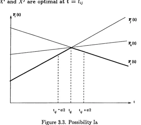
Possibility I : tij is a b rea k p o in t

Two subcases arise depending on if Fi{tij) = Fj{tij) = z{tij) or not. la) X ' and a re op tim al a t t = tij

Figure 3.3. Possibility la

X ' and X^ are optimal at t = tij. Ff(t) is not equal to Fj{t) for t different than tij so that is a breakpoint of the optimal trajectory.

Since there can be only one breakpoint in an interval of length e, we know that there cannot be any other breakpoints in the interval {tij - £ /2,i,j + e /2]. The solution at t = tij - e/2 is the left optimal solution at t = and corre spondingly, the solution at t = tij + e¡2 \s the right optimal solution at t = and they are both optimal at t = tij. Note that the left-right optimal solutions may or may not be supplied from ( In Figure 3.3, they are ).

(39)

Ib)A^‘ and are not optimal at t = <,·

Figure 3.4. Possibility Ib

X ' and X^ are not optimal at t = tij. However, there is a breakpoint of the optimal trajectory corresponding to optimal solutions at t = tij. Fi{tij) = Fj{tij) > z{tij) implies that there exist indices l,k with {i , j) H = 0 so that the optimal solutions at t = Uj = tik are X ‘, X^. In this case, the solutions at t = tij - e/2 and t = Uj + e/2 are the left-right optimal solutions at t = Uj.

(40)

Possibility II : Uj is not a b rea k p o in t

Two subcases arise depending on if there is a breakpoint within an e/2 neighborhood of or not.

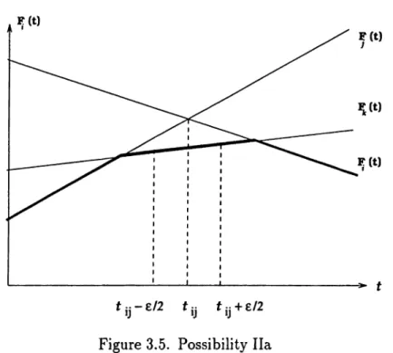
Ila ) No b reak p o in t in th e e /2 neighborhood of t{j

Figure 3.5. Possibility Ila

and X ' are not optimal at t = Neither do we have a breakpoint of the optimal trajectory in the interval [i,j - e / 2,i,j + e /2].

The optimal solution at t = Uj, namely X^ is optimal both at t = - e/2 and t = tij + e /2. Due to Lemma 3, we can conclude that X ’^ is optimal in the interval - e /2,i,j + e:/2] and we do not have any breakpoints in this interval.

(41)

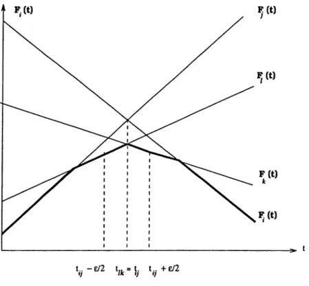
lib) There is a breakpoint in the e / 2 neighborhood of

and X ' are not optimal at t = t{j. We have X* as the optimal solution. However, this solution is not optimal throughout [t,j - e /2,i,y + e /2]. There fore, there is a breakpoint either on the left or on the right of Uj but not both since we cannot have two breakpoints in an interval of length e (Lemma 2).

Ilbi : There is a breakpoint to the right of

In this subcase the solution X'’ is still optimal at t = t{j - e/2 but another solution, X ‘ in Figure 3.6, is optimal at t = tij -|- e / 2. So, there is a breakpoint in the interval {tij, tij -f e/2).

(42)

Ilbii : There is a breakpoint to the left of t i j

In this subcase the solution at t = + e/2 is optimal but another solution, in Figure 3.7, is optimal at t = tij - e /2. So, there is a breakpoint in the interval {tij — e /2, t,j).

Figure 3.7. Possibility Ilbii

In both subcases of Ilb, we have exactly one breakpoint in the interval {tij - e /2,t,j + e /2).

In all of the above explained possibilities, we can decompose the problem into two by dividing the time interval [0,u] into two subintervals: [/, t,j] and [t,j, u].

All of the above possibilities may arise if we are using an e from (0,^). However, we will not have Possibility II b) if e is chosen from (0,^') or (0, LB) because there cannot be more than one intersection point, i.e. an element of r , in an interval of length e when e < L B < i < i'. If we exclude Possibility II b) for a moment, then for all of the remaining cases the course of action is the same. We find the left solution X~ and f{ X~ ,t) at t = — e/2 and the right solution X'*' and f{X'^,t) at t = tij + e /2 . Then we divide the current interval [/,u] into two subintervals and continue with the newly generated intervals in like manner.

(43)

If we use € G (0,£), we would have Possibility II b). In Possibility II b) i, we find the intersection point of Fi{t) and i^fc(t), namely Then, we find the solution at t = tij + {Uk - = (ilk + to )/2 to determine the left_right optimal solution at t = tij. Using Lemma 2 and the fact that {tik - tij) < e/2, we can conclude that the solution at t = {tik + Uj)/2 is optimal in [Lj.iijt]. We divide the problem into two corresponding to intervals and [ijit,«].

Similarly, in Possibility II b) ii, we find the breakpoint of P/(t) and Fk{t), namely tik, find the solution at t = tik + (Lj - tik)/2 = [Uj + tik)¡2 and con clude that this solution is optimal in the interval [tik, tij]. We divide the problem into two as that of finding the trajectory in intervals [/, t/jt] and [<,jjn]·

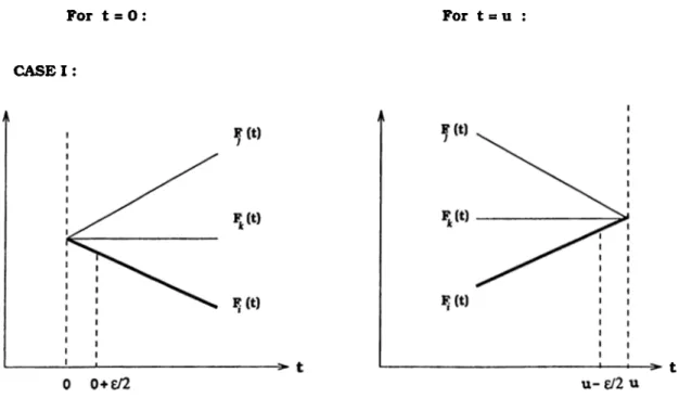
There only remains the course of action to be taken at the end points of the interval [0,u] to be investigated. Let be an optimal solution found at 0 ( or u ). When w'e are solving a static problem at the end points, we have one of the three possibilities shown in Figure 3.8.

For t = O : For t = u ;

CASE I

(44)

CHAPTER 3. MEDIANS WITH LINEAR WEIGHTS 32 For t = 0 : For t = u C A S E D : C A S E D !: 0

o+e/2

^ t Figure 3.8 Continues

As is evident from the figures, we need to compare the objective values of solutions at t = 0 and t = e / 2 o r t = u and t = u-e/2. If they are the same, then the solution at t = e/2 is the right optimal solution at t = 0 or the solution at t = u-e/2 is the left optimal solution at t = u ( Cases I and II ). If they are different, we take the course of action that we would take for Possibility Ilb) i at t = 0 and Possibility II b) ii at t = u ( Case I I I ). All three cases are possible regardless of how we choose e ( from (0,LB) or (0,£), as there is no bound on the length between a breakpoint and an end point of the time interval [0,u] ).

(45)

Based on the above analysis, the proposed algorithm constructs the tra jectory of pjnedian problems with linear weights by solving 0{q) static mul timedian problems. The algorithm is general in the sense that we could find the trajectory of p_ML(t) and p_MML(t) problems both on trees and cyclic networks with the algorithm. Furthermore, if we can find a lower bound to the length between two adjacent breakpoints and if we have an algorithm to find the minimum function at a fixed time point in 0 (r) time ( r is a function of the problem input ), we could find the lower envelope of exponentially many induced linear functions in 0 (r9) time using this algorithm.

3.2.2 T he A lgorith m

We will first explain the algorithm on a small example and then give the formal statement. Let us consider a p_MML(t) problem on a tree network with n = 9 existing facilities and p = 4 new facilities to be located over the interval [0,100].

Weights between new facilities, Vjjt(t) = Ojk + Pjk* t :

j\k 1 2 3 4 1 O+Ot 0”h3t l “l-3t O-hOt 2 0+3t O+Ot 5“t-t 2“h2t 3 l+ 3t 5+t 0“|“0t 4-bt 4 0-t"0t 2-|-2t 4-1-t O-bOt h = { (1,2),(1,3),(2,3),(2,4),(3,4)}

Weights between new and existing facilities, i/;,j(t) = a{j + bij* t :

j\i 1 2 3 4 5 6 7 8 9

1 6 + t O-f-Ot 5-|“2t 3"f-2t 04“0t 0-b4t 0-j“0t 0“|“0t O-bOt 2 O-bOt 3“["t O-bOt 3"f“2t 5"}-t 0-b3t O-bOt O-j-Ot 0“l“0t 3 O-fOt 0“h0t 0“l“0t O-bOt 2H“2t O+Ot 1+ t 0-[-3t 2“t*3t 4 O-bOt O-bOt 0H“0t O-bOt O-bOt 2-bt 5+ 2t 0“h0t 3“l“2t h = { (1,1),(1,3),(1,4),(1,6),(2,2),(2,4),(2,5),(2,6),

Analysis of multimedian problems on time dependent networks

ANALYSIS OF MULTIMEDIAN

PROBLEMS ON TIME

DEPENDENT NETWORKS

By

F. Sibel Salman

July, 1994

Нс

ABSTRACT

ANALYSIS OF MULTIMEDIAN PROBLEMS ON TIME

DEPENDENT NETWORKS

F. Sibel Salman

M.S. in Industrial Engineering

Advisor: Assoc. Prof. Barbaros

Tansel

July, 1994

ÖZET

ZAMANA BAĞIMLI SERİMLERDE ÇOK TESİSLİ YER

SEÇİMİ PROBLEMİNİN ANALİZİ

F. Sibel Salman

Endüstri Mühendisliği, Yüksek Lisans

Dcimşman: Doç. Dr. Barbaros Ç. Tansel

Temmuz 1994

ACKNOWLEDGMENTS

Contents

List of Figures

List of Tables

Chapter 1

Introduction

1.1

M otivation

1.2

D ynam ic Location Problem s in th e Literature

1.3

Scope o f th e T hesis

Chapter 2

Multimedian Problems on Time

Dependent Networks

2.1

T he Clcissical p_M edian P roblem

2.2

T he p_M edian w ith M utual C om m unication P rob­

lem

2.3

T im e D ependen t p_M edian Problem s

=

+

ELi+i

Chapter 3

Medians with Linear Weights :

Trajectory Construction

3.1

p_M edian P rob lem s w ith Linear W eights

X)

=

d"

3.2

Trajectory C on struction

3.2.1

Prelim inaries

o+e/2

3.2.2

T he A lgorith m

T he p_M edian w ith M utual C om m unication P rob