CLASSIFICATION OF
HISTOPATHOLOGICAL CANCER STEM
CELL IMAGES IN H&E STAINED LIVER
TISSUES
a thesis submitted to
the graduate school of engineering and science
of bilkent university
in partial fulfillment of the requirements for
the degree of
master of science
in
electrical and electronics engineering
By
Cem Emre Akba¸s
March 2016
CLASSIFICATION OF HISTOPATHOLOGICAL CANCER STEM CELL IMAGES IN H&E STAINED LIVER TISSUES
By Cem Emre Akba¸s March 2016
We certify that we have read this thesis and that in our opinion it is fully adequate, in scope and in quality, as a thesis for the degree of Master of Science.
A. Enis C¸ etin(Advisor)
U˘gur G¨ud¨ukbay
Kasım Ta¸sdemir
Approved for the Graduate School of Engineering and Science:
Levent Onural
ABSTRACT
CLASSIFICATION OF HISTOPATHOLOGICAL
CANCER STEM CELL IMAGES IN H&E STAINED
LIVER TISSUES
Cem Emre Akba¸s
M.S. in Electrical and Electronics Engineering Advisor: A. Enis C¸ etin
March 2016
Microscopic images are an essential part of cancer diagnosis process in modern medicine. However, diagnosing tissues under microscope is a time-consuming task for pathologists. There is also a significant variation in pathologists’ decisions on tissue labeling. In this study, we developed a computer-aided diagnosis (CAD) system that classifies and grades H&E stained liver tissue images for pathologists in order to speed up the cancer diagnosis process. This system is designed for H&E stained tissues, because it is cheaper than the conventional CD13 stain.
The first step is labeling the tissue images for classification purposes. CD13 stained tissue images are used to construct ground truth labels, because in H&E stained tissues cancer stem cells (CSC) cannot be observed by naked eye.
Feature extraction is the next step. Since CSCs cannot be observed by naked eye in H&E stained tissues, we need to extract distinguishing texture features. For this purpose, 20 features are chosen from nine different color spaces. These features are fed into a modified version of Principal Component Analysis (PCA) algorithm, which is proposed in this thesis. This algorithm takes covariance ma-trices of feature mama-trices of images instead of pixel values of images as input. Images are compared in the eigenspace and classifies them according to the an-gle between them. It is experimentally shown that this algorithm can achieve 76.0% image classification accuracy in H&E stained liver tissues for a three-class classification problem.
Scale invariant feature transform (SIFT), local binary patterns (LBP) and directional feature extraction algorithms are also utilized to classify and grade H&E stained liver tissues. It is observed in the experiments that these features
iv
do not provide meaningful information to grade H&E stained liver tissue images. Since our aim is to speed up the cancer diagnosis process, computation-ally efficient versions of proposed modified PCA algorithm are also proposed. Multiplication-free cosine-like similarity measures are employed in the modified PCA algorithm and it is shown that some versions of the multiplication-free similarity measure based modified PCA algorithm produces better classification accuracies than the standard modified PCA algorithm. One of the proposed multiplication-free similarity measures achieves 76.0% classification accuracy in our dataset containing 454 images of three classes.
¨
OZET
H&E BOYANMIS
¸ KARAC˙I ˘
GER DOKULARINDA
H˙ISTOPATOLOJ˙IK KANSER K ¨
OK H ¨
UCRE
˙IMGELER˙IN˙IN SINIFLANDIRILMASI
Cem Emre Akba¸s
Elektrik-Elektronik M¨uhendisli˘gi, Y¨uksek Lisans Tez Danı¸smanı: A. Enis C¸ etin
Mart 2016
Mikroskopik g¨or¨unt¨uler modern tıpta kanser tanısının ¨onemli bir par¸casıdır. Fakat, dokulara mikroskop altında tanı koymak patologlar i¸cin olduk¸ca zaman alıcı ve yorucu bir i¸stir. Bu tezde, pataloglar i¸cin kanser tanı sistemini hızlandırma amacıyla H&E boyanmı¸s doku imgelerini sınıflandıran ve derecelendiren bilgisa-yar bilgisa-yardımlı bir tanı sistemi geli¸stirdik. Bu sistem H&E boyanmı¸s dokular i¸cin dizayn edildi, ¸c¨unk¨u bu boya yaygın olarak kullanılan CD13 boyasından daha d¨u¸s¨uk maliyetlidir.
Bu sistemimizde ilk adım doku imgelerinin etiketlenmesidir. CD13 boyanmı¸s imgeler yer ger¸cekli˘gi etiketlerinin olu¸sturulması i¸cin kullanılmı¸stır, ¸c¨unk¨u H&E boyanmı¸s dokularda kanser k¨ok h¨ucreleri ¸cıplak g¨ozle (KKH) g¨or¨ulememektedir. Sistemimizdeki sonraki adım ¨oznitelik ¸cıkarımıdır. KKH’ler H&E boyanmı¸s dokularda ¸cıplak g¨ozle g¨or¨ulemedi˘gi i¸cin ¨or¨unt¨u ayırt edici ¨oznitelikler ¸cıkarmamız gerekmektedir. Bu ama¸cla dokuz farklı renk uzayından 20 ¨oznitelik se¸cilmi¸stir. Bu ¨oznitelikler, bu ¸calı¸smada ¨onerilen de˘gi¸stirilmi¸s Ana Bile¸senler Analizi (PCA) algoritmasına girdi olarak verilmi¸stir. Bu algoritma, imgelerin piksel de˘gerleri yerine imgelerin ¨oznitelik matrislerinin ortak de˘gi¸sinti matrislerini girdi olarak kullanır. mgeler ¨ozuzayda (eigenspace) kar¸sıla¸stırır ve aralarındaki a¸cıya g¨ore sınıflandırılır. Bu algoritmanın ¨u¸c sınıf H&E boyanmı¸s karaci˘ger dokularını sınıflandırma probleminde 76.0% imge sınıflandırma ba¸sarısı sa˘gladı˘gı deneysel sonu¸clarla g¨osterilmi¸stir.
¨
Oznitelik ¸cıkarmak i¸cin ¨ol¸cekten ba˘gımsız ¨oznitelik d¨on¨u¸s¨um¨u (SIFT), yerel ikili ¨or¨unt¨uler (LBP) ve y¨onsel ¨oznitelik ¸cıkarma algoritmalarından da fay-dalanılmı¸stır. Deneylerde, bu ¨oznitelik ¸cıkarma algoritmalarının H&E boyanmı¸s
vi
karaci˘ger doku imgelerinin derecelendirilmesi i¸cin anlamlı bilgi sa˘glayamadı˘gı g¨or¨ulm¨u¸st¨ur.
Bu ¸calı¸smada amacımız kanser tanı s¨urecini hızlandırmak oldu˘gu i¸cin, de˘gi¸stirilmi¸s PCA algoritmasının hesap y¨uk¨u d¨u¸s¨ur¨ulm¨u¸s versiyonları da ¨ oner-ilmi¸stir. C¸ arpmasız kosin¨us benzeri benzerlik ¨ol¸c¨uleri de˘gi¸stirilmi¸s PCA al-goritmasında kullanılmı¸stır ve ¸carpmasız benzerlik ¨ol¸c¨us¨u tabanlı de˘gi¸stirilmi¸s PCA algoritmalarının bazılarının ¸carpmaya dayalı standart de˘gi¸stirilmi¸s PCA al-goritmasından daha iyi sınıflandırma sonu¸cları ¨uretti˘gi g¨or¨ulm¨u¸st¨ur. Onerilen¨ ¸carpmasız benzerlik ¨ol¸c¨ulerinden birisi de˘gi¸stirilmi¸s PCA algoritmasında kul-lanıldı˘gında ¨u¸c sınıfa ait 454 imge i¸ceren bir veri setinde %76.0 sınıflandırma ba¸sarısı elde edilmi¸stir.
Anahtar s¨ozc¨ukler : PCA, Doku Derecelendirme, Or¨¨ unt¨u Sınıflandırma, G¨or¨unt¨u Sınıflandırma.
“Simplicity is the ultimate sophistication.” - Leonardo da Vinci
Acknowledgement
My first and foremost thanks goes to my family. None of this would have hap-pened without them and I am deeply indebted for their continuous and uncon-ditional support. Besides all, they also took major parts in my life-long learning process:
• My mother taught me how to read at the age of three and initiated my learning journey.
• My brother helped me establish a solid analytical thinking background. • My father introduced me modern science and molecular biology at my early
ages.
I would also like to express my deepest gratitude to:
• My thesis advisor Dr. Ahmet Enis C¸ etin for sharing his invaluable academic and life experiences with me.
• My thesis committee members Dr. U˘gur G¨ud¨ukbay and Dr. Kasım Ta¸sdemir for their valuable feedback.
• T ¨UB˙ITAK for the scholarship. This thesis is partially funded by T ¨UB˙ITAK 113E069 and T ¨UB˙ITAK 213E032 project.
• Dr. Ece Akhan G¨uzelcan and Dr. Reng¨ul C¸ etin Atalay for providing CD13 and H&E stained liver and lung tissue image datasets.
• Dr. Kasım Ta¸sdemir for sharing his precious research experience with me and for his contributions to my research.
• My close friend Erdem Karag¨ul for magically appearing at ‘that’ moments. • My close friend Hazal Demiral for having visionary answers for all my
x
• My close friend Okan Demir for enlightening coffee talks mostly at the toughest moments of the graduate life.
• My close friends Sinem Meleknur Sertel, Alican Bozkurt, Fırat Yılmaz, Altu˘g Baykal, Eren Hala¸c, G¨okmen Can, Bilgehan I¸sıklı, Alper Yo˘gurt, Mustafa ¨Utk¨ur, Egemen ¨Ozdamar, Ekrem Bilgehan Uyar and Ya¸sar Daysal for their support and good memories.
• Past and present members of Bilkent Signal Processing Group: Ali-can Bozkurt, Mohammad Tofighi, H¨useyin Aslano˘glu, Onur Yorulmaz, O˘guzhan O˘guz, Musa Tun¸c Arslan and Rasim Akın Sevimli.
• Mirco de Govia for his inspirational tunes. The support of his music was quite exceptional.
• Alican Bozkurt (again) for everything.
The story goes that Picasso was sitting in a Paris caf´e when an admirer ap-proached and asked if he would do a quick sketch on a paper napkin. Picasso politely agreed, swiftly executed the work and handed back the napkin, but not before asking for a rather significant amount of money. The admirer was shocked: “How can you ask for so much? It took you five minutes to draw this!” “No”, Picasso replied, “It took me 40 years plus five minutes”. Of course, it took me 24.5 years plus 9 months to develop my research background and produce this thesis. All my previous teachers, classmates and friends who took part in my learning journey deserve my final thanks.
Contents
1 Introduction 1
1.1 Feature Extraction . . . 2
1.2 Microscopic Image Classification . . . 3
2 CSC Image Classification with Modified Principal Component Analysis Algorithm 4 2.1 Modified PCA Algorithm . . . 9
2.2 Feature Extraction from Color Spaces . . . 10
2.3 Experimental Results . . . 12
2.4 Comparison With SIFT Features . . . 20
2.4.1 Experimental Results with Single-Channel Features . . . . 23
2.4.2 Experimental Results with Multi-Channel Features . . . . 25
2.5 Comparison With LBP Features . . . 33
CONTENTS xii
3 CSC Classification in H&E Stained Liver Tissue Images Using
Directional Feature Extraction Algorithms 38
3.1 Directional Filtering . . . 38
3.2 Experimental Results . . . 44
4 Modified PCA Algorithm Based CSC Classification Using Multiplication-free Cosine-Like Similarity Measures 47 4.1 Experimental Results . . . 51
4.1.1 Results with c0 Similarity Measure . . . 51
4.1.2 Results with c1 Similarity Measure . . . 54
4.1.3 Results with c2 Similarity Measure . . . 56
4.1.4 Results with c3 Similarity Measure . . . 59
4.1.5 Results with c4 Similarity Measure . . . 61
4.1.6 Summary . . . 64
4.2 Application on H&E Stained Lung Tissue Image Dataset . . . 65
List of Figures
2.1 CD13 (left) and H&E (right) stained successive tissue layer images
of the same patient. . . 5
2.2 Sample H&E images according to calculated CSC levels. . . 6
2.3 Microscopic Image of an H&E Stained Normal (CSC density= 0%) Liver Tissue Image . . . 7
2.4 Microscopic Image of an H&E Stained Grade I (CSC density< 5%) Liver Tissue Image . . . 7
2.5 Microscopic Image of an H&E Stained Grade II (CSC density> 5%) Liver Tissue Image . . . 8
2.6 Eigenvalues of the Training Set When Query Image is Taken From the First Patient of Grade I Image Set . . . 10
2.7 3-Channel (RGB) Liver Image . . . 11
2.8 R Channel of an H&E Stained RGB Liver Tissue Image . . . 12
2.9 G Channel of an H&E Stained RGB Liver Tissue Image . . . 13
2.10 B Channel of an H&E Stained RGB Liver Tissue Image . . . 14
LIST OF FIGURES xiv
2.12 U Channel of an H&E Stained YUV Liver Tissue Image . . . 15
2.13 V Channel of an H&E Stained YUV Liver Tissue Image . . . 16
2.14 H Channel of an H&E Stained HE Liver Tissue Image . . . 16
2.15 E Channel of an H&E Stained HE Liver Tissue Image . . . 17
2.16 S Channel of an H&E Stained HSV Liver Tissue Image . . . 17
2.17 Obtaining Keypoint Descriptor from Image Gradients for Eight Orientation Bins . . . 20
2.18 Keypoints Found by SIFT Algorithm on Y Channel of an H&E Stained Grade II Liver Tissue Image . . . 22
2.19 Circular (8, 2) Neighborhood LBP Feature Extraction for one Pixel 33 3.1 Frequency responses of directional and rotated filters, for θ = 0◦, ±26.56◦, ±45◦, ±63.43◦, 90◦ . . . 43
List of Tables
2.1 Confusion Matrix of Three-Class 3-NN Modified PCA Image Clas-sification Using Color Space Features . . . 18 2.2 Confusion Matrix of Three-Class 3-NN Modified PCA Patient
Classification Using Color Space Features . . . 18 2.3 Confusion Matrix of Two-Class (Healthy vs. Cancerous) 3-NN
Modified PCA Image Classification Using Color Space Features . 18 2.4 Confusion Matrix of Two-Class (Healthy vs. Cancerous) 3-NN
Modified PCA Patient Classification Using Color Space Features . 18 2.5 Confusion Matrix of Two-Class (Grade I vs. Grade II) 3-NN
Mod-ified PCA Image Classification Using Color Space Features . . . . 19 2.6 Confusion Matrix of Two-Class (Grade I vs. Grade II) 3-NN
Mod-ified PCA Patient Classification Using Color Space Features . . . 19 2.7 Confusion Matrix of Three-Class 3-NN Modified PCA Image
Clas-sification Using SIFT Features of Y Channel . . . 23 2.8 Confusion Matrix of Three-Class 3-NN Modified PCA Patient
LIST OF TABLES xvi
2.9 Confusion Matrix of Two-Class (Healthy vs. Cancerous) 3-NN Modified PCA Image Classification Using SIFT Features of Y Channel . . . 24 2.10 Confusion Matrix of Two-Class (Healthy vs. Cancerous) 3-NN
Modified PCA Patient Classification Using SIFT Features of Y Channel . . . 24 2.11 Confusion Matrix of Two-Class (Grade I vs. Grade II) 3-NN
Mod-ified PCA Image Classification Using SIFT Features of Y Channel 24 2.12 Confusion Matrix of Two-Class (Grade I vs. Grade II) 3-NN
Mod-ified PCA Patient Classification Using SIFT Features of Y Channel 25 2.13 Confusion Matrix of Three-Class 3-NN Modified PCA Image
Clas-sification Using SIFT Features of Y, H and E Channels . . . 26 2.14 Confusion Matrix of Three-Class 3-NN Modified PCA Patient
Classification Using SIFT Features of Y, H and E Channels . . . . 26 2.15 Confusion Matrix of Two-Class (Healthy vs. Cancerous) 3-NN
Modified PCA Image Classification Using SIFT Features of Y, H and E Channels . . . 26 2.16 Confusion Matrix of Two-Class (Healthy vs. Cancerous) 3-NN
Modified PCA Patient Classification Using SIFT Features of Y, H and E Channels . . . 27 2.17 Confusion Matrix of Two-Class (Grade I vs. Grade II) 3-NN
Mod-ified PCA Image Classification Using SIFT Features of Y, H and E Channels . . . 27 2.18 Confusion Matrix of Two-Class (Grade I vs. Grade II) 3-NN
Mod-ified PCA Patient Classification Using SIFT Features of Y, H and E Channels . . . 28
LIST OF TABLES xvii
2.19 Confusion Matrix of Three-Class 3-NN Modified PCA Image Clas-sification Using SIFT Features of Y, H, E, R, G and B Channels . 28 2.20 Confusion Matrix of Three-Class 3-NN Modified PCA Patient
Classification Using SIFT Features of Y, H, E, R, G and B Channels 29 2.21 Confusion Matrix of Two-Class (Healthy vs. Cancerous) 3-NN
Modified PCA Image Classification Using SIFT Features of Y, H, E, R, G and B Channels . . . 29 2.22 Confusion Matrix of Two-Class (Healthy vs. Cancerous) 3-NN
Modified PCA Patient Classification Using SIFT Features of Y, H, E, R, G and B Channels . . . 30 2.23 Confusion Matrix of Two-Class (Grade I vs. Grade II) 3-NN
Mod-ified PCA Image Classification Using SIFT Features of Y, H, E, R, G and B Channels . . . 30 2.24 Confusion Matrix of Two-Class (Grade I vs. Grade II) 3-NN
Mod-ified PCA Patient Classification Using SIFT Features of Y, H, E, R, G and B Channels . . . 31 2.25 Confusion Matrix of Three-Class 3-NN Modified PCA Image
Clas-sification Using SIFT Features of R, G and B Channels . . . 31 2.26 Confusion Matrix of Three-Class 3-NN Modified PCA Patient
Classification Using SIFT Features of R, G and B Channels . . . 31 2.27 Confusion Matrix of Two-Class (Healthy vs. Cancerous) 3-NN
Modified PCA Image Classification Using SIFT Features of R, G and B Channels . . . 31 2.28 Confusion Matrix of Two-Class (Healthy vs. Cancerous) 3-NN
Modified PCA Patient Classification Using SIFT Features of R, G and B Channels . . . 32
LIST OF TABLES xviii
2.29 Confusion Matrix of Two-Class (Grade I vs. Grade II) 3-NN Mod-ified PCA Image Classification Using SIFT Features of R, G and B Channels . . . 32 2.30 Confusion Matrix of Two-Class (Grade I vs. Grade II) 3-NN
Mod-ified PCA Patient Classification Using SIFT Features of R, G and B Channels . . . 32 2.31 Confusion Matrix of Three-Class 3-NN Modified PCA Image
Clas-sification Using LBP Features . . . 35 2.32 Confusion Matrix of Three-Class 3-NN Modified PCA Patient
Classification Using LBP Features . . . 35 2.33 Confusion Matrix of Two-Class (Healthy vs. Cancerous) 3-NN
Modified PCA Image Classification Using LBP Features . . . 35 2.34 Confusion Matrix of Two-Class (Healthy vs. Cancerous) 3-NN
Modified PCA Patient Classification Using LBP Features . . . 36 2.35 Confusion Matrix of Two-Class (Grade I vs. Grade II) 3-NN
Mod-ified PCA Image Classification Using LBP Features . . . 36 2.36 Confusion Matrix of Two-Class (Grade I vs. Grade II) 3-NN
Mod-ified PCA Patient Classification Using LBP Features . . . 36
3.1 Directional and rotated filters for θ = {0◦, ±26.56◦, ±45◦, ±63.43◦, 90◦} 39
3.2 Confusion Matrix of Three-Class 3-NN Modified PCA Image Clas-sification with Directional Filtering Features Extracted from 3 Scales 44 3.3 Confusion Matrix of Three-Class 3-NN Modified PCA Patient
Classification with Directional Filtering Features Extracted from 3 Scales . . . 44
LIST OF TABLES xix
3.4 Confusion Matrix of Two-Class (Cancerous vs. Normal) 3-NN Modified PCA Image Classification with Directional Filtering Fea-tures Extracted from 3 Scales . . . 45 3.5 Confusion Matrix of Two-Class (Cancerous vs. Normal) 3-NN
Modified PCA Patient Classification with Directional Filtering Features Extracted from 3 Scales . . . 45 3.6 Confusion Matrix of Two-Class (Grade I vs. Grade II) 3-NN
Mod-ified PCA Image Classification with Directional Filtering Features Extracted from 3 Scales . . . 46 3.7 Confusion Matrix of Two-Class (Grade I vs. Grade II) 3-NN
Modi-fied PCA Patient Classification with Directional Filtering Features Extracted from 3 Scales . . . 46
4.1 Confusion Matrix of Three-Class 3-NN c0 Similarity Measure Based Modified PCA Image Classification . . . 51 4.2 Confusion Matrix of Three-Class 3-NN c0 Similarity Measure
Based Modified PCA Patient Classification . . . 52 4.3 Confusion Matrix of Two-Class (Cancerous vs. Normal) 3-NN c0
Similarity Measure Based Modified PCA Image Classification . . . 52 4.4 Confusion Matrix of Two-Class (Cancerous vs. Normal) 3-NN c0
Similarity Measure Based Modified PCA Patient Classification . . 53 4.5 Confusion Matrix of Two-Class (Grade I vs. Grade II) 3-NN c0
Similarity Measure Based Modified PCA Image Classification . . . 53 4.6 Confusion Matrix of Two-Class (Grade I vs. Grade II) 3-NN c0
LIST OF TABLES xx
4.7 Confusion Matrix of Three-Class 3-NN c1 Similarity Measure Based Modified PCA Image Classification . . . 54 4.8 Confusion Matrix of Three-Class 3-NN c1 Similarity Measure
Based Modified PCA Patient Classification . . . 54 4.9 Confusion Matrix of Two-Class (Cancerous vs. Normal) 3-NN c1
Similarity Measure Based Modified PCA Image Classification . . . 55 4.10 Confusion Matrix of Two-Class (Cancerous vs. Normal) 3-NN c1
Similarity Measure Based Modified PCA Patient Classification . . 55 4.11 Confusion Matrix of Two-Class (Grade I vs. Grade II) 3-NN c1
Similarity Measure Based Modified PCA Image Classification . . . 56 4.12 Confusion Matrix of Two-Class (Grade I vs. Grade II) 3-NN c1
Similarity Measure Based Modified PCA Patient Classification . . 56 4.13 Confusion Matrix of Three-Class 3-NN c2 Similarity Measure
Based Modified PCA Image Classification . . . 56 4.14 Confusion Matrix of Three-Class 3-NN c2 Similarity Measure
Based Modified PCA Patient Classification . . . 57 4.15 Confusion Matrix of Two-Class (Cancerous vs. Normal) 3-NN c2
Similarity Measure Based Modified PCA Image Classification . . . 57 4.16 Confusion Matrix of Two-Class (Cancerous vs. Normal) 3-NN c2
Similarity Measure Based Modified PCA Patient Classification . . 58 4.17 Confusion Matrix of Two-Class (Grade I vs. Grade II) 3-NN c2
Similarity Measure Based Modified PCA Image Classification . . . 58 4.18 Confusion Matrix of Two-Class (Grade I vs. Grade II) 3-NN c2
LIST OF TABLES xxi
4.19 Confusion Matrix of Three-Class 3-NN c3 Similarity Measure Based Modified PCA Image Classification . . . 59 4.20 Confusion Matrix of Three-Class 3-NN c3 Similarity Measure
Based Modified PCA Patient Classification . . . 59 4.21 Confusion Matrix of Two-Class (Cancerous vs. Normal) 3-NN c3
Similarity Measure Based Modified PCA Image Classification . . . 60 4.22 Confusion Matrix of Two-Class (Cancerous vs. Normal) 3-NN c3
Similarity Measure Based Modified PCA Patient Classification . . 60 4.23 Confusion Matrix of Two-Class (Grade I vs. Grade II) 3-NN c3
Similarity Measure Based Modified PCA Image Classification . . . 61 4.24 Confusion Matrix of Two-Class (Grade I vs. Grade II) 3-NN c3
Similarity Measure Based Modified PCA Patient Classification . . 61 4.25 Confusion Matrix of Three-Class 3-NN c4 Similarity Measure
Based Modified PCA Image Classification . . . 61 4.26 Confusion Matrix of Three-Class 3-NN c4 Similarity Measure
Based Modified PCA Patient Classification . . . 62 4.27 Confusion Matrix of Two-Class (Cancerous vs. Normal) 3-NN c4
Similarity Measure Based Modified PCA Image Classification . . . 62 4.28 Confusion Matrix of Two-Class (Cancerous vs. Normal) 3-NN c4
Similarity Measure Based Modified PCA Patient Classification . . 63 4.29 Confusion Matrix of Two-Class (Grade I vs. Grade II) 3-NN c4
Similarity Measure Based Modified PCA Image Classification . . . 63 4.30 Confusion Matrix of Two-Class (Grade I vs. Grade II) 3-NN c4
LIST OF TABLES xxii
4.31 Overall 3-NN Image Classification Accuracies Using Modified PCA Method with 6 Different Similarity Measures. Best Result in Each Case is Presented in Bold Fonts. . . 64 4.32 Overall 3-NN Patient Classification Accuracies Using Modified
PCA Method with 6 Different Similarity Measures. Best Result in Each Case is Presented in Bold Fonts. . . 64 4.33 Confusion Matrix of Two-Class (Grade I vs. Grade II) 3-NN c4
Similarity Measure Based Modified PCA Image Classification . . . 65 4.34 Confusion Matrix of Two-Class (Grade I vs. Grade II) 3-NN c4
Chapter 1
Introduction
In cancer diagnosis and grading process, analysis of microscopic images is still the most reliable method. However, grading liver tissue images under microscope is a time-consuming and tiring task. There is also a significant variation in patholo-gists’ decisions on tissue labeling [1–4]. Therefore, there may occur human-based errors due to tiredness. Our main motivation to develop a computer-aided diagno-sis (CAD) system is to speed up the cancer diagnodiagno-sis process, since time is a very critical issue in cancer diagnosis and treatment. Another important advantage of using a CAD is that its grading and classification results are reproducible.
CAD enables us to have a two stage decision mechanism. First, our algorithm makes a decision. Then, the pathologist checks our algorithm’s decision and makes the final decision. This two stage decision mechanism help the pathologist make more correct decisions about the cancer diagnosis and tissue grading.
In the early 1990’s, digital mammography was one of the first developed CAD system [5, 6]. Since that day, CAD has been actively used in detection of breast cancer in the United States of America [7]. This interest obviously boosted the research in medical imaging and digital diagnosis systems.
1.1
Feature Extraction
Feature vectors are used to represent a given image or give a specific information about a given image. In most of the image classification problems, feature vectors are used instead of pixel values of the image in the classification algorithms. Depending on the classification task, some features may require more emphasis and some may require less. If the aim is to detect red objects in a given image, it is expected that more features are extracted from the red channel of RGB color space and less features are extracted from other channels. Hence, more useful information about the image can be obtained for the specific classification task by choosing features properly.
In this thesis, the main challenge is that cancer stem cells (CSC) cannot be ob-served by naked eye in H&E stained liver tissues, although our task is to classify images according to their CSC ratios. Therefore, feature extraction gained promi-nence, since other distinguishing features in the images need to be exploited. This leads to an image classification based on their texture differences. We use discrete derivative of color histograms as features along with standard color histograms in Chapter 2. Additionally, pixel thresholding is applied to color histograms in order to avoid extracting features from empty or meaningless areas of a given image. When there are more than one feature vector, feature vectors can be concatenated to have one single feature vector or they can be cascaded to form a 2-D feature matrix. Covariance matrix of the feature matrix can also be used to obtain a more compact and smaller form of the feature matrix, which reduces the processing time and speeds up the classification process.
Scale invariant feature transform (SIFT), local binary patterns (LBP) and di-rectional feature extraction algorithms are also used to obtain features from a given image in different directions in Chapter 3 [8]. The importance of choos-ing the right feature extraction method can clearly be seen by comparchoos-ing the classification accuracies in Chapter 2 and Chapter 3.
1.2
Microscopic Image Classification
Image classification is the next step after feature extraction. In this thesis, we focus on diagnosis and grading of H&E stained liver tissue images. We propose a modified version of Principal Component Analysis (PCA) algorithm, which takes covariance matrices of feature matrices of images instead of pixel values of images as input for texture classification. This algorithm is similar to the well-known eigenface algorithm [9, 10], which compares images in the eigenspace.
In Chapter 2, color space features are fed into the modified PCA algorithm. In Chapter 3, directional feature set is used by modified PCA algorithm. In Chapter 4, distance calculation in modified PCA algorithm is replaced by multiplication-free operators to reduce the computational cost of the CAD system. In this case, color space features are used. In Chapter 5, obtained results are discussed and final remarks are made.
Chapter 2
CSC Image Classification with
Modified Principal Component
Analysis Algorithm
H&E stain is a cost effective histopathological technique [11–23]. It is hard to distinguish CSCs in H&E images, unlike CD13 stained images. CSCs can easily be distinguished in CD13 images, however it is an expensive stain. Therefore, a method that can classify H&E images considering their CSC densities would be more feasible and accessible. In this chapter, a classification method that classifies H&E images according to their CSC densities will be developed.
First, a brief explanation of the acquisition process of the histopathological images from the patients is given. In the acquisition process first, a sample tissue is taken from a patient and it is sliced in very thin layers. The successive layers look very similar, but they are not exactly the same. Since a stained layer cannot be stained again with another stain, it is not possible to have both CD13 and H&E stained versions of the same tissue layer. Therefore, successive layers are stained with CD13 and H&E stains assuming that they have almost the same visual properties (see Figure 2.1). Based on this assumption, CSC densities are calculated using CD13 stained layers to construct ground truth labels for
corresponding H&E images.
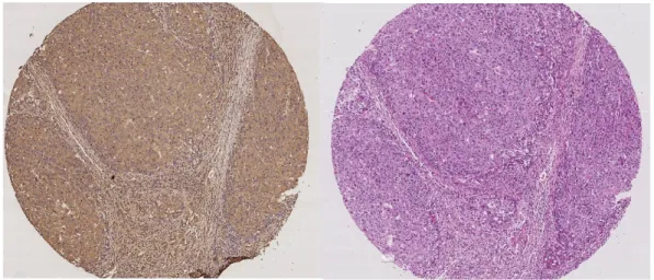
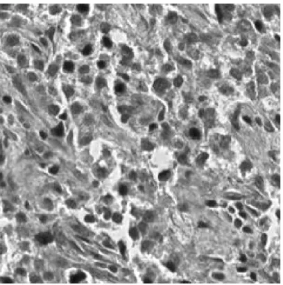
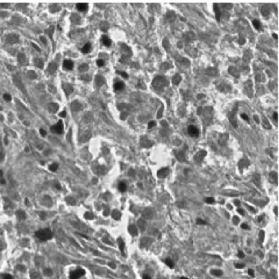
Figure 2.1: CD13 (left) and H&E (right) stained successive tissue layer images of the same patient.
In Figure 2.1, the successive layer images of the same tissue stained with CD13 and H&E are shown. CSC density in the chosen region is defined as the ratio of number of CSCs to number of all cells. This density is calculated on an arbitrarily chosen image region of CD13 stained tissue layer. The calculated density is assumed to be the same in the corresponding region of the successive H&E stained layer. The CSC density in the chosen region is calculated as follows:
CSC Ratio = P CSC
P All Cells (2.1)
A grading scheme is defined according to CSC percentages. If the CSC Per-centage is less than 5%, that region is labeled as Grade I. If it is greater than or equal to 5%, it is labeled as Grade II. If it is equal to 0%, it is labeled as normal, meaning that it contains no CSC. It is important to note that CD13 stained images are only used in labeling corresponding H&E tissue images. They are not involved in any part of the proposed method except extracting ground truth data.
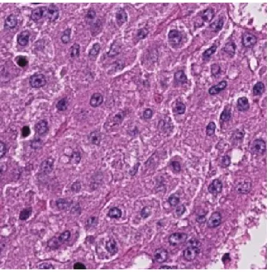
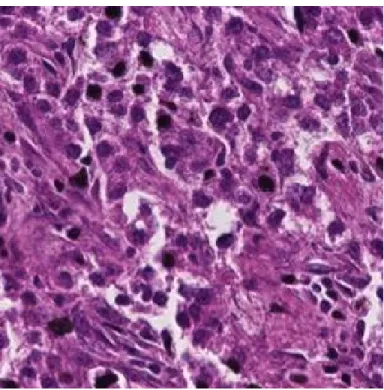
Figure 2.2: Sample H&E images according to calculated CSC levels.
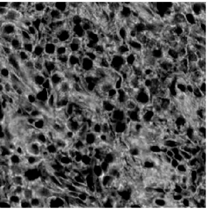
In Figure 2.2, sample images of H&E stained normal, Grade I and Grade II tissue layers are shown. It is observed that the amount of darker regions increases as CSC ratio increases. This fact causes a significant pattern and color difference between three classes. Feature extraction methods are applied to these H&E images and obtained feature matrices are fed into the modified PCA algorithm for classification.
The proposed classification algorithm is similar to well-known eigenface algo-rithm [9]. Unlike conventional eigenface algoalgo-rithm, covariance matrix of color histograms instead of pixel values are fed into the modified PCA algorithm. His-tograms of the image, that of thresholded image, first and second order discrete derivative of them in various color spaces are used to construct the feature ma-trix. Our aim is to distinguish three classes of liver images; Grade I (Figure 2.4), Grade II (Figure 2.5), normal (Figure 2.3).
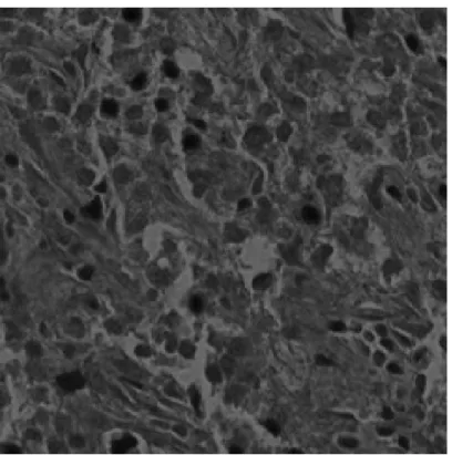
Figure 2.3: Microscopic Image of an H&E Stained Normal (CSC density= 0%) Liver Tissue Image
Figure 2.4: Microscopic Image of an H&E Stained Grade I (CSC density< 5%) Liver Tissue Image
Figure 2.5: Microscopic Image of an H&E Stained Grade II (CSC density> 5%) Liver Tissue Image
2.1
Modified PCA Algorithm
In this section, we propose a modified version of Principal Component Analysis (PCA) algorithm, which takes covariance matrices of feature matrices of images instead of pixel values of images as input for texture classification. In the proposed modified PCA algorithm, average covariance matrix of training set is calculated as follows: CV = 1 N N X i=1 FiT × Fi (2.2)
In Equation (2.2), N is the number of images in training set and Fi is the feature
matrix of ith image. Covariance matrix (C
V) of training set images is a 128x128
matrix. Eigenvalues λkand eigenvectors ukof CV are computed. The steps below
are followed for comparing two images:
(i) Let γ be the average of columns of FmT× Fm and ζ be average of columns of
FT
n × Fn, where m is index of the reference image and n is index of the compared
image.
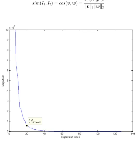
(ii) The reference image is projected onto the ‘cell space’ by multiplying γ by the first 20 vectors of uk(20 eigenvectors corresponding to 20 largest eigenvalues),
as in Equation (2.3) where µγ is the mean of γ. In Figure 2.6, it is shown that
largest 20 eigenvalues of the training set is significantly larger than the remaining eigenvalues.
vk = uTk(γ − µγ), k = 1, 2, ..., 20 (2.3)
Similarly, the compared image is projected onto the ‘cell space’ by multiply-ing ζ by the first 20 vectors of uk (20 eigenvectors corresponding to 20 largest
eigenvalues), as in Equation (2.4) where µζ is the mean of ζ.
(iii) The similarity between two images is defined as follows: sim(I1, I2) = cos(v, w) =
< v · w > kvk2kwk2
(2.5)
Figure 2.6: Eigenvalues of the Training Set When Query Image is Taken From the First Patient of Grade I Image Set
2.2
Feature Extraction from Color Spaces
The difference of three classes is their CSC ratio. Due to their higher CSC ratio, Grade II images have a tendency to have more dark regions than Grade I and normal images. Therefore, the proposed feature matrix utilizes color space histograms. All images in our dataset are acquired in RGB color space and converted to YUV, HE [17] and HSV color spaces for feature extraction. The
feature matrix is as follows:
F = [hist(R) hist(Rt) hist(G) hist(Gt) hist(B) hist(Bt) hist(Y )
hist(Y )0 hist(Yt) hist(U ) hist(U )0 hist(U )00 hist(V ) hist(V )0
hist(V )00 hist(H) hist(Ht) hist(E) hist(S) hist(St)]T
(2.6) ,where R is red channel, G is green channel, B is blue channel of RGB color space
Figure 2.7: 3-Channel (RGB) Liver Image
respectively; Y is luminance channel, U and V are chrominance channels of YUV color space respectively; H is Hematoxylin channel, E is Eosin channel of HE color space respectively and S is saturation channel of HSV colorspace. The hist(·) function computes a 128-bin histogram of a given input. The hist(·)0 function denotes the first order discrete derivative of hist(·), hist(·)00 function denotes the second order discrete derivative of hist(·) and (·t) denotes pixel thresholding in
that specified channel. Pixel thresholding is utilized to extract more descriptive features from darker regions1. In the experiments, this threshold is empirically
selected as 200. In R, G, B, Y, U, V and E channels, pixel values greater than 200 are discarded. However, in H and S channels, pixel values smaller than 200 are discarded. Therefore, more representative features of ‘darker regions’ are extracted. In Equation 2.6, hist(·) function produces a column vector of size 128 × 1 in the range [0,255]. A feature matrix F of size 20x128 for each image is obtained by cascading each histogram output..
Figure 2.8: R Channel of an H&E Stained RGB Liver Tissue Image
2.3
Experimental Results
Our dataset consists of three classes of H&E stained liver images; Grade I (119 images taken from 17 patients), Grade II (151 images taken from 17 patients) and normal (184 images taken from 9 patients) tissue images. three-nearest neighbor classification is used to determine the class of a test image. Instead of leave-one-image-out strategy, leave-one-patient-out strategy is used; since each patient has more than one image. The term ‘patient classification accuracy’ is defined in order
Figure 2.9: G Channel of an H&E Stained RGB Liver Tissue Image to make a decision about patients. In order to classify a patient, majority voting is employed among the decisions of the patient’s images. The test set is circulated to cover all instances and contains one image at each iteration. Throughout this thesis, recall (2.7), precision (2.8) and overall accuracy (2.9) are used to measure the performance of designed CAD systems.
Recall = P T rueP ositives
P T rueP ositives + P F alseN egatives (2.7)
P recision = P T rueP ositives
P T rueP ositives + P F alseP ositives (2.8)
OverallAccuracy = P T rueP ositives + P T rueN egatives
P T otalP opulation (2.9)
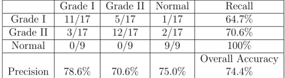
Figure 2.10: B Channel of an H&E Stained RGB Liver Tissue Image achieved in three-class image and patient classification respectively. It is impor-tant to emphasize that normal image classification accuracy is 89.8%. It is also observed that image and patient classification accuracies of the same cases may differ significantly due to the majority voting applied in the patient classification. In Tables 2.3 and 2.4, Grade I and Grade II images together constitute the cancerous class. In this case, overall image classification is 93.0%. Another important point is that cancerous image classification accuracy is 93.3% and normal image classification accuracy is 90.2%.
In Tables 2.5 and 2.6, normal images are excluded from the dataset and clas-sification is performed among cancerous images. In this case, image clasclas-sification accuracy is 70.4% and patient classification accuracy is 73.5%.
It is experimentally observed that modified PCA algotihm with color space features achieves significant accuracies in two-class and three-class classification and grading problem.
Figure 2.11: Y Channel of an H&E Stained YUV Liver Tissue Image
Figure 2.13: V Channel of an H&E Stained YUV Liver Tissue Image
Figure 2.15: E Channel of an H&E Stained HE Liver Tissue Image
Table 2.1: Confusion Matrix of Three-Class 3-NN Modified PCA Image Classifi-cation Using Color Space Features
Grade I Grade II Normal Recall
Grade I 70/119 41/119 8/119 58.8%
Grade II 38/151 102/151 11/151 67.5%
Normal 12/184 5/184 167/184 90.8%
Overall Accuracy
Precision 58.3% 68.9% 89.8% 74.7%
Table 2.2: Confusion Matrix of Three-Class 3-NN Modified PCA Patient Classi-fication Using Color Space Features
Grade I Grade II Normal Recall
Grade I 11/17 5/17 1/17 64.7%
Grade II 3/17 12/17 2/17 70.6%
Normal 0/9 0/9 9/9 100%
Overall Accuracy
Precision 78.6% 70.6% 75.0% 74.4%
Table 2.3: Confusion Matrix of Two-Class (Healthy vs. Cancerous) 3-NN Modi-fied PCA Image Classification Using Color Space Features
Cancerous Normal Recall
Cancerous 252/270 18/270 93.3%
Normal 18/184 166/184 90.2%
Overall Accuracy
Precision 93.3% 90.2% 92.1%
Table 2.4: Confusion Matrix of Two-Class (Healthy vs. Cancerous) 3-NN Modi-fied PCA Patient Classification Using Color Space Features
Cancerous Normal Recall
Cancerous 31/34 3/34 91.2%
Normal 0/0 9/9 100%
Overall Accuracy
Table 2.5: Confusion Matrix of Two-Class (Grade I vs. Grade II) 3-NN Modified PCA Image Classification Using Color Space Features
Grade I Grade II Recall
Grade I 77/119 42/119 64.7%
Grade II 38/151 113/151 74.8%
Overall Accuracy
Precision 67.0% 72.9% 70.4%
Table 2.6: Confusion Matrix of Two-Class (Grade I vs. Grade II) 3-NN Modified PCA Patient Classification Using Color Space Features
Grade I Grade II Recall
Grade I 11/17 6/17 64.7%
Grade II 3/17 14/17 82.4%
Overall Accuracy
2.4
Comparison With SIFT Features
Scale Invariant Feature Transform (SIFT) is a widely used feature extraction method for object recognition problems [24–26]. This algorithm aims to extract scale and rotation invariant features of images. Previous studies show that this algorithm performs robust object recognition. In this section, we will extract SIFT features from our histopathological image dataset and compare them with color space histogram features on our three-class texture classification problem.
In this thesis, Lowe’s SIFT implementation and source codes are used [27]. This implementation is composed of four steps; scale-space extrema detection, keypoint localization, orientation assignment and keypoint descriptor. In the first step, difference-of-Gaussian function is used to identify potential points that are invariant to scale and orientation. At keypoint localization stage, keypoints are selected among all candidate points based on measures of their stability. Then, one or more orientations are assigned to each keypoint location based on local image gradient directions for orientation assignment. In the last step, histogram of image gradients is computed for eight orientation bins and stored in the feature vector, which is the vector representation of the keypoint descriptor. The feature vector contains magnitudes of the elements of histogram of image gradients. A sample image gradients and keypoint descriptor are shown in Figure 2.172.
Figure 2.17: Obtaining Keypoint Descriptor from Image Gradients for Eight Orientation Bins
In the experiments, histograms of gradients are taken from a 4 × 4 descriptor window computed from a 16 × 16 sample array around the keypoint. Since, histograms of image gradients are computed in eight orientation bins, resulting feature vector is 128-element. A CSC image has N keypoints, so a feature matrix is of size N × 128 is obtained by cascading all feature vectors of keypoints. This feature matrix is fed into the modified PCA algorithm and 3-NN classification is performed.
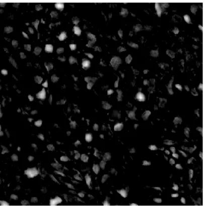
In Figure 2.18, keypoints found by Lowe’s SIFT algorithm on Y channel of an H&E stained liver tissue image is shown. Keypoints are mostly found on darker regions as desired.
(a) A Sample H&E Stained Grade II Liver Tissue in RGB Color Space
(b) Keypoints Found by SIFT Algorithm on Y Channel of an H&E Stained Grade II Liver Tissue Image
Figure 2.18: Keypoints Found by SIFT Algorithm on Y Channel of an H&E Stained Grade II Liver Tissue Image
2.4.1
Experimental Results with Single-Channel Features
The same dataset in Section 2.3 is used which has 454 images of three classes. First, SIFT features are extracted from Y channels of input images, because SIFT algorithm extract features from single-channel image data. Classification and grading performance of the modified PCA algorithm using SIFT features will be observed and compared with the results obtained by color space features.
Table 2.7: Confusion Matrix of Three-Class 3-NN Modified PCA Image Classifi-cation Using SIFT Features of Y Channel
Grade I Grade II Normal Recall
Grade I 34/119 65/119 20/119 28.6%
Grade II 60/151 45/151 46/151 29.8%
Normal 11/184 37/184 136/184 73.9%
Overall Accuracy
Precision 32.4% 30.6% 67.3% 47.4%
Table 2.8: Confusion Matrix of Three-Class 3-NN Modified PCA Patient Classi-fication Using SIFT Features of Y Channel
Grade I Grade II Normal Recall
Grade I 4/17 11/17 2/17 23.5%
Grade II 9/17 3/17 5/17 17.6%
Normal 0/9 0/9 9/9 100%
Overall Accuracy
Precision 30.8% 21.4% 56.3% 37.2%
As seen in Tables 2.7 and 2.8, 47.4% image classification accuracy and 37.2% patient classification accuracy is obtained by SIFT features. These accuracies are far smaller than the accuracies obtained by color space features (Tables 2.1 and 2.2). In this case, the best recognition performance is observed in normal class images.
In Tables 2.9 and 2.10, image classification accuracy is 75.5% and patient clas-sification accuracy is 81.4%. In this case, it is shown that significant clasclas-sification
Table 2.9: Confusion Matrix of Two-Class (Healthy vs. Cancerous) 3-NN Modi-fied PCA Image Classification Using SIFT Features of Y Channel
Cancerous Normal Recall
Cancerous 208/270 62/270 77.0%
Normal 49/184 135/184 73.4%
Overall Accuracy
Precision 80.9% 68.5% 75.5%
Table 2.10: Confusion Matrix of Two-Class (Healthy vs. Cancerous) 3-NN Mod-ified PCA Patient Classification Using SIFT Features of Y Channel
Cancerous Normal Recall
Cancerous 27/34 7/34 79.4%
Normal 1/9 8/9 88.9%
Overall Accuracy
Precision 96.4% 53.3% 81.4%
accuracies can be obtained by SIFT features, but these results are not comparable to the results obtained by color space features (Tables 2.3 and 2.4).
Table 2.11: Confusion Matrix of Two-Class (Grade I vs. Grade II) 3-NN Modified PCA Image Classification Using SIFT Features of Y Channel
Grade I Grade II Recall
Grade I 50/119 69/119 42.0%
Grade II 67/151 84/151 55.6%
Overall Accuracy
Precision 42.7% 54.9% 49.6%
In Tables 2.11 and 2.12, cancerous tissues are graded in two-class case. Im-age classification accuracy is 49.6% and patient classification accuracy is 41.2%. These results are not comparable to the results obtained by color space features (Tables 2.11 and 2.12).
Considering all three cases of classification and grading of H&E stained liver tissue images, it is experimentally observed that SIFT features can distinguish
Table 2.12: Confusion Matrix of Two-Class (Grade I vs. Grade II) 3-NN Modified PCA Patient Classification Using SIFT Features of Y Channel
Grade I Grade II Recall
Grade I 6/17 11/17 35.3%
Grade II 9/17 8/17 47.1%
Overall Accuracy
Precision 60.0% 42.1% 41.2%
cancerous and normal tissues (two-class healthy vs. cancerous case). However, they do not produce good results in two-class grading of cancerous tissue images and three-class classification case.
2.4.2
Experimental Results with Multi-Channel Features
The same dataset in Section 2.3 is used which has 454 images of three classes. In this subsection, SIFT features are extracted from various color channels sep-arately and then extracted SIFT feature matrices are cascaded horizontally to form the feature matrix. In the experiments we analyze three multi-channel cases using combinations of Y channel of YUV color space, H channel and E channel of HE color space and R channel, G channel and B channel of RGB color space. Classification and grading performance of the modified PCA algorithm us-ing multi-channel SIFT features will be observed and compared with the results obtained by single-channel SIFT features and histograms of color space features. First, features are extracted from Y, H and E channels and obtained results are compared with the results obtained in single-channel case.
As seen in Tables 2.13 and 2.14, 53.7% image classification accuracy and 44.2% patient classification accuracy is obtained by multi-channel SIFT features ex-tracted from Y, H and E channels. These accuracies are better than the accura-cies obtained by single-channel SIFT features extracted from Y channel (Tables 2.7 and 2.8). In three-class case, using multi-channel SIFT features improves the
Table 2.13: Confusion Matrix of Three-Class 3-NN Modified PCA Image Classi-fication Using SIFT Features of Y, H and E Channels
Grade I Grade II Normal Recall
Grade I 38/119 64/119 17/119 31.9%
Grade II 64/151 60/151 27/151 39.7%
Normal 9/184 29/184 146/184 79.3%
Overall Accuracy
Precision 34.2% 39.2% 76.8% 53.7%
Table 2.14: Confusion Matrix of Three-Class 3-NN Modified PCA Patient Clas-sification Using SIFT Features of Y, H and E Channels
Grade I Grade II Normal Recall
Grade I 4/17 10/17 3/17 23.5%
Grade II 9/17 6/17 2/17 35.3%
Normal 0/9 0/9 9/9 100%
Overall Accuracy
Precision 30.8% 62.5% 64.3% 44.2%
classification performance of the system.
Table 2.15: Confusion Matrix of Two-Class (Healthy vs. Cancerous) 3-NN Mod-ified PCA Image Classification Using SIFT Features of Y, H and E Channels
Cancerous Normal Recall
Cancerous 208/270 62/270 77.0%
Normal 49/184 135/184 73.4%
Overall Accuracy
Precision 80.9% 68.5% 75.5%
In Tables 2.15 and 2.16, image classification accuracy is 75.5% and patient classification accuracy is 81.4%. In this case, obtained results are the same as the results obtained by single-channel SIFT features (Tables 2.9 and 2.10).
In Tables 2.17 and 2.18, image classification accuracy is 49.6% and patient classification accuracy is 41.2%. In this case, obtained results are the same as the
Table 2.16: Confusion Matrix of Two-Class (Healthy vs. Cancerous) 3-NN Mod-ified PCA Patient Classification Using SIFT Features of Y, H and E Channels
Cancerous Normal Recall
Cancerous 27/34 7/34 79.4%
Normal 1/9 8/9 88.9%
Overall Accuracy
Precision 96.4% 53.3% 81.4%
Table 2.17: Confusion Matrix of Two-Class (Grade I vs. Grade II) 3-NN Modified PCA Image Classification Using SIFT Features of Y, H and E Channels
Grade I Grade II Recall
Grade I 50/119 69/119 42.0%
Grade II 67/151 84/151 55.6%
Overall Accuracy
Precision 42.7% 54.9% 49.6%
results obtained by single-channel SIFT features (Tables 2.11 and 2.12).
In multi-channel case of SIFT that uses Y, H and E channels for feature ex-traction, it is observed that it outperforms single-channel case in three-class clas-sification and it produces same results as the single-channel case in two-class classifications. Therefore, six color channels are used in the next multi-channel case.
In the second multi-channel case of SIFT, features are extracted from Y, H, E, R, G and B channels and obtained results are compared with the results obtained in single-channel case and previous multi-channel case.
As seen in Tables 2.19 and 2.20, 53.7% image classification accuracy and 44.2% patient classification accuracy is obtained by multi-channel SIFT features ex-tracted from Y, H, E, R, G and B channels. These classification accuracies are better than the accuracies obtained by single-channel SIFT features extracted from Y channel (Tables 2.7 and 2.8) and the same as the previous multi-channel case.
Table 2.18: Confusion Matrix of Two-Class (Grade I vs. Grade II) 3-NN Modified PCA Patient Classification Using SIFT Features of Y, H and E Channels
Grade I Grade II Recall
Grade I 6/17 11/17 35.3%
Grade II 9/17 8/17 47.1%
Overall Accuracy
Precision 60.0% 42.1% 41.2%
Table 2.19: Confusion Matrix of Three-Class 3-NN Modified PCA Image Classi-fication Using SIFT Features of Y, H, E, R, G and B Channels
Grade I Grade II Normal Recall
Grade I 38/119 64/119 17/119 31.9%
Grade II 64/151 60/151 27/151 39.7%
Normal 9/184 29/184 146/184 79.3%
Overall Accuracy
Precision 34.2% 39.2% 76.8% 53.7%
In Tables 2.21 and 2.22, image classification accuracy is 75.5% and patient classification accuracy is 81.4%. These classification accuracies are better than the accuracies obtained by single-channel SIFT features extracted from Y channel (Tables 2.9 and 2.10) and the same as the previous multi-channel case.
In Tables 2.23 and 2.24, image classification accuracy is 49.6% and patient classification accuracy is 41.2%. These classification accuracies are better than the accuracies obtained by single-channel SIFT features extracted from Y channel (Tables 2.11 and 2.12) and the same as the previous multi-channel case.
In multi-channel implementation of SIFT that extracts features from six color channels (Y, H, E, R, G, B), it is observed that it produces better results than the single-channel case. However, it produces the same results as the previous multi-channel case that utilizes three channels (Y, H, E). Therefore, in the next multi-channel case, three color channels are used.
Table 2.20: Confusion Matrix of Three-Class 3-NN Modified PCA Patient Clas-sification Using SIFT Features of Y, H, E, R, G and B Channels
Grade I Grade II Normal Recall
Grade I 4/17 10/17 3/17 23.5%
Grade II 9/17 6/17 2/17 35.3%
Normal 0/9 0/9 9/9 100%
Overall Accuracy
Precision 30.8% 62.5% 64.3% 44.2%
Table 2.21: Confusion Matrix of Two-Class (Healthy vs. Cancerous) 3-NN Mod-ified PCA Image Classification Using SIFT Features of Y, H, E, R, G and B Channels
Cancerous Normal Recall
Cancerous 208/270 62/270 77.0%
Normal 49/184 135/184 73.4%
Overall Accuracy
Precision 80.9% 68.5% 75.5%
and B channels and obtained results are compared with the results obtained in single-channel case and previous multi-channel cases.
As seen in Tables 2.25 and 2.26, 56.4% image classification accuracy and 48.8% patient classification accuracy is obtained by multi-channel SIFT features ex-tracted from R, G and B channels. These classification accuracies are better than the accuracies obtained in all previous SIFT based three-class cases. How-ever, they are not better than the accuracies obtained by color space features (Tables 2.1 and 2.2).
In Tables 2.27 and 2.28, image classification accuracy is 78.9% and patient clas-sification accuracy is 86.1%. These clasclas-sification accuracies are better than the accuracies obtained in all previous SIFT based ‘cancerous or not’ cases. However, they are not better than the accuracies obtained by color space features (Tables 2.3 and 2.4).
Table 2.22: Confusion Matrix of Two-Class (Healthy vs. Cancerous) 3-NN Mod-ified PCA Patient Classification Using SIFT Features of Y, H, E, R, G and B Channels
Cancerous Normal Recall
Cancerous 27/34 7/34 79.4%
Normal 1/9 8/9 88.9%
Overall Accuracy
Precision 96.4% 53.3% 81.4%
Table 2.23: Confusion Matrix of Two-Class (Grade I vs. Grade II) 3-NN Modified PCA Image Classification Using SIFT Features of Y, H, E, R, G and B Channels
Grade I Grade II Recall
Grade I 50/119 69/119 42.0%
Grade II 67/151 84/151 55.6%
Overall Accuracy
Precision 42.7% 54.9% 49.6%
In Tables 2.29 and 2.30, image classification accuracy is 49.6% and patient classification accuracy is 41.2%. These classification accuracies are better than the accuracies obtained by single-channel SIFT features extracted from Y channel (Tables 2.11 and 2.12) and the same as the previous multi-channel two-class grading cases.
Briefly, the best classification accuracies are obtained with multi-channel SIFT features that are extracted from R, G and B channels. However, these classifica-tion accuracies are not better than the accuracies obtained by color space features.
Table 2.24: Confusion Matrix of Two-Class (Grade I vs. Grade II) 3-NN Modified PCA Patient Classification Using SIFT Features of Y, H, E, R, G and B Channels
Grade I Grade II Recall
Grade I 6/17 11/17 35.3%
Grade II 9/17 8/17 47.1%
Overall Accuracy
Precision 60.0% 42.1% 41.2%
Table 2.25: Confusion Matrix of Three-Class 3-NN Modified PCA Image Classi-fication Using SIFT Features of R, G and B Channels
Grade I Grade II Normal Recall
Grade I 40/119 63/119 16/119 33.6%
Grade II 58/151 70/151 23/151 46.4%
Normal 11/184 27/184 146/184 79.3%
Overall Accuracy
Precision 36.7% 43.8% 78.9% 56.4%
Table 2.26: Confusion Matrix of Three-Class 3-NN Modified PCA Patient Clas-sification Using SIFT Features of R, G and B Channels
Grade I Grade II Normal Recall
Grade I 5/17 10/17 2/17 29.4%
Grade II 8/17 7/17 2/17 41.2%
Normal 0/9 0/9 9/9 100%
Overall Accuracy
Precision 38.5% 41.2% 69.2% 48.8%
Table 2.27: Confusion Matrix of Two-Class (Healthy vs. Cancerous) 3-NN Mod-ified PCA Image Classification Using SIFT Features of R, G and B Channels
Cancerous Normal Recall
Cancerous 219/270 51/270 81.1%
Normal 45/184 139/184 75.5%
Overall Accuracy
Table 2.28: Confusion Matrix of Two-Class (Healthy vs. Cancerous) 3-NN Mod-ified PCA Patient Classification Using SIFT Features of R, G and B Channels
Cancerous Normal Recall
Cancerous 29/34 5/34 85.3%
Normal 1/9 8/9 88.9%
Overall Accuracy
Precision 96.7% 61.5% 86.1%
Table 2.29: Confusion Matrix of Two-Class (Grade I vs. Grade II) 3-NN Modified PCA Image Classification Using SIFT Features of R, G and B Channels
Grade I Grade II Recall
Grade I 51/119 68/119 42.9%
Grade II 68/151 83/151 55.0%
Overall Accuracy
Precision 42.9% 55.0% 49.6%
Table 2.30: Confusion Matrix of Two-Class (Grade I vs. Grade II) 3-NN Modified PCA Patient Classification Using SIFT Features of R, G and B Channels
Grade I Grade II Recall
Grade I 6/17 11/17 35.3%
Grade II 9/17 8/17 47.1%
Overall Accuracy
2.5
Comparison With LBP Features
Local Binary Patterns (LBP) is another widely used feature extraction method for texture classification problems [28–32]. This algorithm is known to extract both texture and shape information of a given image. Ahonen’s circular (8, 2) neighborhood LBP model is used in this thesis and it is shown in Figure 2.19.
Figure 2.19: Circular (8, 2) Neighborhood LBP Feature Extraction for one Pixel In this LBP model, an 8-bit binary number is extracted from each pixel. Each pixel is visited and compared with its eight neighbors. Starting form top-left neighbor, if center pixel is greater than or equal to its neighbor ‘1’ is written, otherwise ‘0’ is written to construct the 8-bit feature number. This 8-bit binary number is converted to decimal and stored in the pattern vector. This process is repeated for each pixel in the image. Finally, 128-bin histogram of this pattern vector is computed to form the feature vector. In experiments, we only extracted LBP features from keypoints found by SIFT algorithm in order to reduce compu-tational cost and extract features around cell parts. Eleven LBP feature vectors are extracted from eleven different color spaces as in Equation (2.10).
FLBP = LBPR LBPG LBPB LBPY LBPU LBPV LBPH LBPE LBPHH LBPS LBPV V (2.10)
In Equation (2.10) LBP features are extracted from red channel (LBPR), green
channel (LBPG), and blue channel (LBPB) of RGB space respectively; luminance
channel (LBPY) and chrominance channels (LBPU and LBPV) of YUV space
respectively; Hematoxylin channel (LBPH) and Eosin channel (LBPE) of HE
space [17] respectively; hue channel (LBPHH), saturation channel (LBPS) and
value channel (LBPV V) of HSV space respectively. Resulting feature matrix
FLBP is of size 11 × 128 and fed into the modified PCA algorithm to perform
classification and grading of H&E stained liver tissue images.
2.5.1
Experimental Results
The same dataset in Section 2.3 is used which has 454 images of three classes. Classification and grading performance of the modified PCA algorithm using LBP features will be observed and compared with the results obtained by color space features.
As seen in Tables 2.31 and 2.32, designed classifier tends to classify all images as Grade I. Therefore, image classification accuracy is 24.9% and patient classifi-cation accuracy is 37.2%. Although almost all of the Grade I images are retrieved
Table 2.31: Confusion Matrix of Three-Class 3-NN Modified PCA Image Classi-fication Using LBP Features
Grade I Grade II Normal Recall
Grade I 113/119 0/119 6/119 95.0%
Grade II 144/151 0/151 7/151 0.0%
Normal 184/184 0/184 0/184 0.0%
Overall Accuracy
Precision 25.6% 0.0% 0.0% 24.9%
Table 2.32: Confusion Matrix of Three-Class 3-NN Modified PCA Patient Clas-sification Using LBP Features
Grade I Grade II Normal Recall
Grade I 16/17 0/17 1/17 94.1%
Grade II 16/17 0/17 1/17 0.0%
Normal 9/9 0/9 0/9 0.0%
Overall Accuracy
Precision 39.0% 0.0% 0.0% 37.2%
correctly, Grade I class accuracy is 25.6% due to a high number of false positives. Next, a two-class classification will be performed to classify normal and cancerous liver tissue images.
Table 2.33: Confusion Matrix of Two-Class (Healthy vs. Cancerous) 3-NN Mod-ified PCA Image Classification Using LBP Features
Cancerous Normal Recall
Cancerous 257/270 13/270 95.2%
Normal 184/184 0/184 0.0%
Overall Accuracy
Precision 58.3% 0.0% 56.6%
In Tables 2.33 and 2.34, designed classifier tends to classify all images as cancer-ous. In this case, image classification accuracy is 56.6% and patient classification accuracy is 74.4%. Almost all of the cancerous images are retrieved correctly, but
Table 2.34: Confusion Matrix of Two-Class (Healthy vs. Cancerous) 3-NN Mod-ified PCA Patient Classification Using LBP Features
Cancerous Normal Recall
Cancerous 32/34 2/34 94.1%
Normal 9/0 0/9 0.0%
Overall Accuracy
Precision 78.0% 0.0% 74.4%
cancerous class accuracy is 58.3% due to a high number of false positives. It is ob-served that LBP features does not provide meaningful information to distinguish cancerous and normal tissues.
Table 2.35: Confusion Matrix of Two-Class (Grade I vs. Grade II) 3-NN Modified PCA Image Classification Using LBP Features
Grade I Grade II Recall
Grade I 52/119 67/119 43.7%
Grade II 62/151 89/151 58.9%
Overall Accuracy
Precision 45.6% 57.1% 52.2%
Table 2.36: Confusion Matrix of Two-Class (Grade I vs. Grade II) 3-NN Modified PCA Patient Classification Using LBP Features
Grade I Grade II Recall
Grade I 5/17 12/17 29.4%
Grade II 7/17 10/17 58.8%
Overall Accuracy
Precision 41.7% 45.5% 44.1%
In Tables 2.35 and 2.36, cancerous tissues are graded in two-class case. Image classification accuracy is 52.2% and patient classification accuracy is 44.1%. Un-like previous two cases of LBP features, designed classifier does not classify most of the images as a single class. However, classification accuracies are far smaller than the same case with color space features (Tables 2.5, 2.6).
Considering all three cases of classification and grading of H&E stained liver tissue images, it is experimentally observed that LBP features does not extract representative features from normal and cancerous images.
Chapter 3
CSC Classification in H&E
Stained Liver Tissue Images
Using Directional Feature
Extraction Algorithms
In his M.Sc. thesis, Bozkurt introduced directional feature extraction methods for image processing [8]. The purpose of these methods is to extract features of a given image in various directions. In this chapter, directional features from CSC images will be extracted and fed into the modified PCA algorithm for grading classification of H&E stained liver images. Obtained results will be compared with the results in the previous chapter.
3.1
Directional Filtering
Directional filtering framework is developed by Bozkurt in his M.Sc. thesis. In this algorithm, a filter impulse response f0 and filter length N are set initially.
are constructed in several directions and two features are extracted from each direction (mean and standard deviation). Instead of applying directional convo-lution, directional filters are rotated by θ and convolved with the input image. Rotated filters are calculated as in Bozkurt’s thesis. For each directional filter, corresponding rotational filter is calculated by rotating f0 by θ. Directional and
rotated filters for θ = {0◦, ±26.56◦, ±45◦, ±63.43◦, 90◦} is given in Table 3.1.
Table 3.1: Directional and rotated filters for θ = {0◦, ±26.56◦, ±45◦, ±63.43◦, 90◦}
Angle Directional Filter Rotated Filter
−63.43◦ 0 −0.0313 −0.0313 0 0 0 0 0 0 0 0 0 0 0 0 0 0.2813 0.2813 0 0 0 0 0 0 1 0 0 0 0 0 0 0.2813 0.2813 0 0 0 0 0 0 0 0 0 0 0 0 0 −0.0313 −0.0313 0 0 −0.01459 −0.03004 0 0 0 0 0 −0.00451 −0.01475 0.012539 0 0 0 0 0 0.204712 0.336475 0 0 0 0 0 0.084917 1 0.084917 0 0 0 0 0 0.336475 0.204712 0 0 0 0 0 0.012539 −0.01475 −0.00451 0 0 0 0 0 −0.03004 −0.01459 0 −45◦ −0.0625 0 0 0 0 0 0 0 0 0 0 0 0 0 0 0 0.5625 0 0 0 0 0 0 0 1 0 0 0 0 0 0 0 0.5625 0 0 0 0 0 0 0 0 0 0 0 0 0 0 0 −0.0625 0 −0.0085 0 0 0 0 0 −0.0085 −0.05178 −0.00222 0 0 0 0 0 −0.00222 0.329505 0.202284 0 0 0 0 0 0.202284 1 0.202284 0 0 0 0 0 0.202284 0.329505 −0.00222 0 0 0 0 0 −0.00222 −0.05178 −0.0085 0 0 0 0 0 −0.0085 0 −26.56◦ 0 0 0 0 0 0 0 −0.0313 0 0 0 0 0 0 −0.0313 0 0.2813 0 0 0 0 0 0 0.2813 1 0.2813 0 0 0 0 0 0 0.2813 0 −0.0313 0 0 0 0 0 0 −0.0313 0 0 0 0 0 0 0 0 0 0 0 0 0 0 −0.01459 −0.00451 0 0 0 0 0 −0.03004 −0.01475 0.204712 0.084917 0 0 0 0 0.012539 0.336475 1 0.336475 0.012539 0 0 0 0 0.084917 0.204712 −0.01475 −0.03004 0 0 0 0 0 −0.00451 −0.01459 0 0 0 0 0 0 0 0◦ 0 0 0 0 0 0 0 0 0 0 0 0 0 0 0 0 0 0 0 0 0 −0.0625 0 0.5625 1 0.5625 0 −0.0625 0 0 0 0 0 0 0 0 0 0 0 0 0 0 0 0 0 0 0 0 0 0 0 0 0 0 0 0 0 0 0 0 0 0 0 0 0 0 0 0 0 0 −0.0625 0 0.5625 1 0.5625 0 −0.0625 0 0 0 0 0 0 0 0 0 0 0 0 0 0 0 0 0 0 0 0 0 26.56◦ 0 0 0 0 0 0 0 0 0 0 0 0 0 −0.0313 0 0 0 0 0.2813 0 −0.0313 0 0 0.2813 1 0.2813 0 0 −0.0313 0 0.2813 0 0 0 0 −0.0313 0 0 0 0 0 0 0 0 0 0 0 0 0 0 0 0 0 0 0 0 0 0 0 0 0 −0.00451 −0.01459 0 0 0 0.084917 0.204712 −0.01475 −0.03004 0 0.012539 0.336475 1 0.336475 0.012539 0 −0.03004 −0.01475 0.204712 0.084917 0 0 0 −0.01459 −0.00451 0 0 0 0 0 0 0 0 0 0 0 0 45◦ 0 0 0 0 0 0 −0.0625 0 0 0 0 0 0 0 0 0 0 0 0.5625 0 0 0 0 0 1 0 0 0 0 0 0.5625 0 0 0 0 0 0 0 0 0 0 0 −0.0625 0 0 0 0 0 0 0 0 0 0 0 −0.0085 0 0 0 0 0 −0.00222 −0.05178 −0.0085 0 0 0 0.202284 0.329505 −0.00222 0 0 0 0.202284 1 0.202284 0 0 0 −0.00222 0.329505 0.202284 0 0 0 −0.0085 −0.05178 −0.00222 0 0 0 0 0 −0.0085 0 0 0 0 0 63.43◦ 0 0 0 0 −0.0313 −0.0313 0 0 0 0 0 0 0 0 0 0 0 0.2813 0.2813 0 0 0 0 0 1 0 0 0 0 0 0.2813 0.2813 0 0 0 0 0 0 0 0 0 0 0 −0.0313 −0.0313 0 0 0 0 0 0 0 0 −0.03004 −0.01459 0 0 0 0 0.012539 −0.01475 −0.00451 0 0 0 0 0.336475 0.204712 0 0 0 0 0.084917 1 0.084917 0 0 0 0 0.204712 0.336475 0 0 0 0 −0.00451 −0.01475 0.012539 0 0 0 0 −0.01459 −0.03004 0 0 0 0 90◦ 0 0 0 −0.0625 0 0 0 0 0 0 0 0 0 0 0 0 0 0.5625 0 0 0 0 0 0 1 0 0 0 0 0 0 0.5625 0 0 0 0 0 0 0 0 0 0 0 0 0 −0.0625 0 0 0 0 0 0 −0.0625 0 0 0 0 0 0 0 0 0 0 0 0 0 0.5625 0 0 0 0 0 0 1 0 0 0 0 0 0 0.5625 0 0 0 0 0 0 0 0 0 0 0 0 0 −0.0625 0 0 0
features. Therefore, 16 features are obtained from the first scale image for eight directions. In the lower scales, the input image is first decimated by a factor of two both horizontally and vertically. A half sample delay is applied before downsampling, because downsampling operation is shift-variant. After that, the decimated image is filtered by rotated directional filters. Mean and standard deviations of filtered images are used as features. This process can be repeated for further lower scales. At each scale, extracted features constitute a column vector. In multi-scale feature extraction, extracted feature vectors are concatenated to form a 1-D feature vector. In this thesis, features are extracted from three scales that results in a 48 element feature vector for a single input image.
(a) Directional Filter Frequency Response(θ = −63.43◦)
(b) Rotated Filter Frequency Response(θ = −63.43◦)
(c) Directional Filter Frequency Response(θ = −45◦)
(d) Rotated Filter Frequency Response(θ = −45◦)
(e) Directional Filter Frequency Response(θ = −26.56◦)
(f) Rotated Filter Frequency Response(θ = − − 26.56◦)
(g) Directional Filter Frequency Response(θ = 0◦)
(h) Rotated Filter Frequency Response(θ = −0◦)
(i) Directional Filter Frequency Response(θ = 26.56◦)
(j) Rotated Filter Frequency Response(θ = 26.56◦)
(k) Directional Filter Frequency Response(θ = 45◦)
(l) Rotated Filter Frequency Response(θ = 45◦)
(m) Directional Filter Frequency Response(θ = 63.43◦)
(n) Rotated Filter Frequency Response(θ = 63.43◦)
(o) Directional Filter Frequency Response(θ = 90◦)
(p) Rotated Filter Frequency Response(θ = 90◦)
Figure 3.1: Frequency responses of directional and rotated filters, for θ = 0◦, ±26.56◦, ±45◦, ±63.43◦, 90◦