Atomic, electronic, and transport properties of quantum point contacts on graphite surface

ATOMIC, ELECTRONIC, AND TRANSPORT

PROPERTIES OF QUANTUM POINT

CONTACTS ON GRAPHITE SURFACE

A THESIS

SUBMITTED TO THE DEPARTMENT OF PHYSICS

AND THE INSTITUTE OF ENGINEERING AND SCIENCE

OF BILKENT UNIVERSITY

PARTIAL FULFILLMENT OF THE REQUIREMENTS

FOR THE DEGREE OF

MASTER OF SCIENCE

By

Çetin Kılıç

September 1997

ATOMIC, ELECTRONIC, AND TRANSPORT

PROPERTIES OF QUANTUM POINT

CONTACTS ON GRAPHITE SURFACE

A THESIS

SUBMITTED TO THE DEPARTMENT OF PHYSICS AND THE INSTITUTE OF ENGINEERING AND SCIENCE

OF BILKENT UNIVERSITY

IN PARTIAL FULFILLMENT OF THE REQUIREMENTS FOR THE DEGREE OF

MASTER OF SCIENCE

By

Çetin Kılıç

September 1997

Й о З ^ З б ?

7 /" 2 6 / • G 4·

1 cei't,ily J licivc road tJiis iJiesis and lliat in my opinion it is lully adequate, in scope; and in (|ualit3q a,s a dissertation for the degree of Mastei· of Scie'iice.

J certify tliat 1 have read this tliesis and that in my opinion it is fully adequate, in scope and in quality, as a dissertation for the degree of A'lastei· of Science.

1 ci'rtify that 1 have lead tins thesis and tliat in my opinion it is fully adequate, in scope and in quality, as a dissertation (or the degree of Aiaster of Science.

/U ‘ -é ô c — — ^ Assoc, ih'of. Recai l.'dlialtioglir

Approved for the Institute of Rngineering and Science:

Prof. Mehmet

Abstract

ATOMIC, ELECTRONIC, AND TRANSPORT

PROPERTIES OF QUANTUM POINT CONTACTS ON

GRAPHITE SURFACE

Çetin Kılıç

M. S. ill Physics

Supervisor: Prof. Salim Ciraci

Septemlier 1997

111 tins lİK'si.s. the x'ariatioii ol concliictaiice tliroiigli a contact foinied by a liarcl S'JM tip pressing to a graphite substrate is investigated. Our study involves the molecular dynamics simulations to reveal the evolution of the atomic structure during the growth of the contact, and ab initio electronic structure calculations of graphite that, is under the expansive and compressive strain along the [0001] axis, (.'ombining tlie results obtained from these calculations, we propo.se a mechanism to explain the peculiar variation of the conductance. Owing to the layered structure of graphite, the variation of conductance exhibits dramatic differences from those of normal metals. It is predicted that in graphite, the conductance first increases, and then, drops to a lower value with the jDuncture of the atomic plane. This phenomenon repeats quasi-periodically as the tip continues to press on the surface.

K eyw ords: Graphite, ballistic electron transport, quantum point contact, molecular dynamics simulations, band structure calculations

özet

g r a f i t y ü z e y i n d e k i n o k t a s a l k u v a n t u m

DEĞMELERİNİN ATOMİK, ELEKTRONİK VE NAKİL

ÖZELLİKLERİ

Çetin Kılıç

Fizik Yüksok Lisans

Tez Y öneticisi: Prof. Salim Ciraci

Eylül 1997

Bu tezde grafit yüzeyine bastırılan sert SİM tipinin oluşturduğu do'ğrnede iletkenliğin değişimi incelendi. Çalrşınamızda. atomik yapının değıneııiı. büyüme evresinde analiz edilmesi için, moleküler dinamik simülasyonları ve İlasına ve çekme gerilimi altında grafitin temel jırensiplere dayalı elektronik yapı hesapları yapıldı. Bu hesaplardan elde edilen sonuçları birleştirerek grafit değmesinin iletkenliğinin değişimini incelemek üzere bir mekanizma önerdik. Grafitin katmanlı yapısından dolayı elektrik iletkenliğinin (k'ğnıe alanı ile değişimi normal metallere nazaran çok farklılıklar göstermektedir. Grafitte iletkenliğin önce artacağı, daha sonra bir tabakanın tip tarafından delinmesi sonucu düşeceği ve tipin grafiti bastırması sürerken bu olayın periyodik olarak cereyan edeceği öngörüldü.

A n a h ta r

sözcükler: Grafit, balistic elektron nakli, noktasal kuvantum değme, moleküler dinamik simülasyonları, band yapısı hesaplan

Acknowledgement

I would like to express my deepest gratitude to Prof. Dr. .Salim Ciraci for his sujjorvision in research as well as for his interest in my personal problems. It is my indeptness to mention his suggestions, efforts, and beneficial discussions on which this study is based.

I would like to thank .some friends: my office-mate .M. Bayındır for his moral support and helps in pre])a])ering the thesis: H. Mehrez for his comments and his benevolent characteristics in our relationshi]): .Л. Buldum for his helps in developing software; H. Boyacı for his response when computers were not res])onding; Yurt for his moral support.

I acknowledge K. Nordlund for giving immediate response to my questions related to his potential.

Contents

A b s tra c t i

Ö zet i

A cknow ledgem ent i

C o n ten ts i

List of F ig u res iii

List of T ables vi

1 IN T R O D U C T IO N 1

2 T R A N S P O R T IN STM 5

2.1 Transition to Quantum Point Contact... .5

2.1.1 Nearly independent electrode regime 6

2.1.2 Electronic contact regime 7

2.1.3 Point contact r e g im e ... 8 2.2 STM Studies of G rap h ite... 10

3 A T O M IS T IC SIM U L A T IO N S 13

3.1 Atomic Structure of G r a p h ite ... 13 3.2 Interatomic Carbon P o te n tia l... 15 3.3 Molecular Dynamics Simulations ... 25

3.3.1 IJesults and Di.scussioi)... 27

4 SCF PSEU D O PO TEN TIA L CALCULATIONS 32 3.1 Total Eneigy C alnilations... 32 3.2 Band SlrucUire of (ira|)hil,('... 3-3 3.2.1 Eifcx'ts of Uniaxial Distortions on Hand St nut n r e ... 30

5 CONCLUSION 49

List of Figures

2.1 Tunneling current versus distance. 8

2.2 Tunneling current versus e.xcursion... 9 2.3 The measurement of the tip movement and din 1 /(Is. 12

3.1 Graphite in Bernal Structure 14

3.2 The energy of the carbon dimer. 21

3.3 Total energy versus lattice parameter c curve... 22 3.4 The transferability of the interatomic carbon potential. 23 3.5 Binding of a single carbon atom to the graphite lattice. 24 3.0 Variation of the potential energy and convergence of the tempera­

ture during test simulations. 26

3.7 The tip is above B site. 28

3.8 The tip is above H site. 28

3.9 The tip is above .A. site... 29 3.10 The tip punctures the first layer above A site... 30

3.11 Dislocation-induced crashes in first layer. 30

3.12 Formation of the flakes in the first layer... 31 3.13 Second layer is crashed... 31

4.1 The pseudopotential components for carbon. 33

4.2 Brillouin zone of graphite ... 34

4.3 Equilibrium band structure of graphite. 36

4.4 Fermi surface of graphite... 37 4.5 Cuts of Fermi surface of graphite... 37 4.6 Band structure of graphite under uniaxial expansion... 40

-].7 Band structure of graphite under uniaxial coni])ression (c = 0.67-1 A)... 41 4.8 Band structure of graphite under uniaxial compression (c = 4.674

A... 41

4.9 Tight-binding " bands. 44

4.10 Ab iniiio V bands... 45 4.11 Band Structure detailed around Fermi level... 46 4.12 Change in the total density of states with respect to variations of

lattice parameter c... 48 4.13 The valance band density of states from the experimental x-ray

photoemission spectra. 48

List of Tables

4.1 The special points and tlie lines of s_ynnnetry in the Brillouin zone of llie he.xagonal lattice... 3.5 4.2 The energies of a and tt bands at T point relative to the I'ermi

level and the s])littings of tt bands at K point . 38 4.3 The energies of a and tt bands at F point relative to the Fermi

Chapter 1

INTRODUCTION

Atomic size contacts created by a sharp metal ti]r on the sample surface has been a subject of interest, in recent years. In the beginning, the contact has radius of 2~4 A , but it grows l>y ])ushing the t.ip further towards tlie sample. For metallic electron densities the contact diameter {2Hp = 2-4 A ) is in tlie

range of Fenni wcvvelength Xp. In this length scale the le\ el spacing of electrons transversally confined to the contact is approximately 1 eVb Moreover, the discrete structure of the cont act made b}’ atoms becomes pronounced; any change in atomic arrangement and size of the contact can lead to observable variat ions in mechanical and electronic properties. In particular, the two-terminal conductance

G of a contact has shown discontinuous (sudden) variations while the tip is pushed

continuously.^“^ Similar behavior has been obtained recently in a connective neck that was formed by retracting the tip subsequent to a n a n o in d e n ta tio n .A s far as the conductance is concerned, an atomic size cont.act or a connective neck is considered as a constriction with length / smaller than the electron mean free path

le, and with 2Rp ~ Xp. Whether the two terminal ballistic conduct ance of such a

constriction is quantized has been a subject of controversy.®’® While abrupt jumps or falls in the variation of conductance are attributed to the discontinuous change in the cross-section of the contact,^’®’'* several studies favored the quantization.®“®

The point contact spectroscopy has been used earlier to investigate the electron-phonon interaction. The electron transport through a point contact is

(Ч1л т : п i. i N T i i O D r c r i O N

important, not 011I3' lor a Ix'tter miflorstaiicling of meHO.sco[)ic pliysics, Init also for nov('l di'vice applications. Mon'over, various yiiilding· mecliiuiics anti resulting atomic rearrangements during the evolution of tlie contact have Ireen active subject of study. In pai-ticular, the ciuesl.ion whether the continuum meclianics can he applied for tin' formalism of the contacts is under intensive study.

Almost three decades ago, Sharvin'^’ investigated the point contact with / ~ 0 l)y using a semiclassical approach, and showed tliat the conductance is ind('p(Mident of any material properties, but solely determined by the geometry (01· cross-sf'ction S) of the point contact and mean electron density, p of the i ('S(4-voir. d'h(' ('.xpression of contact conductance he ol)tained (which is known as

th(' .Sharvin's conductance) is given by

_ 2e·^

(!.]) /\ccording to Sharvin, f/.s incn'a.sr's linearly with S even if ,S' is much smaller than A;,', 'riiis is, of course, against the uncertainty principle. In the (luanturn 14'gimc tliat is valid for very small 5', = 0 as long as S < Sc] the threshold cross-.secl ion S,· is П.х(ч1 by the uncertainty principh's. Therefore, in the (|uantum regiiiu' (I's deviates liom I he above expri'ssiou. Л realistic atomic-si'/e contact has finite length (/ ф 0), and hence its conductance variation differs from the sc'iniclassical .Sharvin’s conductance.

Ciraci and 'lekman ' (1е\ч‘1ор(ч1 I.Ik' first (piantum tlu’ory for th<‘ conductance of a 1 hree-dimensional (.U)) point contact as a function of/. 'They found that for a uniform and very long (/ ;:§> \ p ) contact (¡(S) exhibits sharp stej) structure having step heights at integer multiples of 2с^//г. This ste])ped structure is smeared out if / < A/.'. 'I'hey attributed the observed sudden changes in the experimental C!{S) ciii've to the smhh'ii (discrete) changi's in S ninh'r the com prt'ssive stress. Recent exp(‘rim(‘nts“ measuring forc(' and c(uidnctance simultaneously, and tin; results of simulations based on moh'cular dynamics calculations'* appear to confirm this thciny. .Several recent studies (Ui the almiiic si/.<· coiit.act.s and c«>nnective necks h.ive eoiil ribiiled :;i,i4iiIic,'iii1 1 1.0 0111 nnderstandiiii', o| the balli.sl.ic coiidilctaiH'e ill metal ((fillai I , \ snmmarv of the reiciil niideistanding on ilie (|iiaiili/.alioii

CHAPTER 1. E^m O D VC nO N

ol ballistic coiKludaiice is pieseiiled hc're. B_v considciing the contact as a const rict ion bet ween t wo elect ron I’eservoirs, the elect ronic st ates are t i-ansxx'rsall}· conhned in 2D, but jU’opagate along the third direction. 'I'lie stat.('s (with coiresjjonding eigenenergies) in the constriction arc e.x])ressed as

Piji Pifi · _{^ij~i — ^‘■|.7 + T.¿Ill} (1.2)

An electron entering the constriction evolves into a current transporting state with ju'opcr enei'g}' and monienturn conservations. Such a state can be e.xpiessed as a linear coiDbinatio]] of For a uniform constriction with / smaller than the mean fiee jrath /, but / > Xp. each current transporting state (having degeneracy

IIij) with Ep < < Ep + cV·^ (V being the bias voltage) can contribute to

the conductance by 2nijC/h. Therefore, a uniform and ideal constiiction would

have G(S) curve that displays the staircase structure with siiarp stej)s. However, wlien I < Xp and atomic structure is irregular; the true G’(.S') curve normally increases with ,S', Init is smeared out and exliibits sudden changes whenever S has a discontinuous growtli. The variation of G with S for a contact between metal tip and sample surlace demonstrates the cjuantization of electronic states in the constriction, but not the ciuantization of ballistic conductance.

The conductance of the point contact generated by sharp tip on t he graphite is found rather peculiar and different from the above picture. In the experiments done at Bilkent,^^ and IBM Zürich Laboratory,*^ it is found that G{s) does not increase with the push of the tip s, but oscillates between two values. So far no understanding has developed for such a behavior, and hence the conductance of the contact formed on the graphite surface has remained a inystery. Graphite has very interesting and directional properties*^’*^; it is an important material for STAi*^ and intercalation process.*^ In addition, graphite is essential for carbon bucky-balls (fullerenes) and nanotubes. Carbon-carbon bonds are very strong within a layer, but interlayer interaction is very w'eak. This anisotropy leads to a very soft Young modulus E, and very small conductance (? (~ 1 i)“ *c77?.) along the direction perpendicular to the layers, w'hereas in layers G (~ 1 x 10“*

CHAPTER 1. INTRODUCTION

strong covalent bonds of which they are made up. The directional behavior is also reflected to the electronic structure making graphite a semimetal with a very narrow Fermi surface.

The strange behavior of the atomic size contact on graphite surface is important for mesoscopic physics, and is investigated in this thesis. This study involves state-of-the-art moleculcir dynamics simulations and ab initio total energy, band, and density of states calculations. The results of energy band calculations yield semimetal to metal transition under uniaxial compression. The indentation of a sharp and hard tip on the graphite surface proceeds discontinuously each time making a puncture on a new graphite layer. Based on these results, we propose a model that successfully explains the peculiar behavior of electron transport through an atomic contact created by an STM tip. Besides, the mechanism revealed in this study can lead to potential device applications.

Chapter 2

TRANSPORT IN SCANNING

TUNNELING MICROSCOPY

2.1

Transition to Quantum Point Contact

Scanning tunneling microscopy (STM) was the first technique which gives the possibility of direct probing of surface structure in real-space, ultimately with atomic resolution. A point-like probe (being kept proximate to the surface) is combined with a piezoelectric drive system to scan the sample, providing local information via vacuum tunneling of electrons. Scanning is performed b\^ several modes operating the tip. Among all, the constant current mode is most commonly used.^'^ In this mode, in order to keep the tunneling current constant, a feedback circuit adjusts the tip height by applying an appropriate voltage V- to the ¿r piezoelectric drive. The lateral tip position {x.,y) is determined by the values 14 and Vy applied to x and y piezoelectric drives, respectively. 14 is recorded with respect to the variations of 14 and I4 , and 14(14,14) i^ translated into z{x,y) giving the topographic image of the surface.

The tip position can correspond to three different regimes^*’’^' depending upon the tip-surface separation .s as described in the following subsections. The first two are included since they occur prior to the point contact as s gets smaller.

CHAPTER 2. TRANSPORT IN STM

2.1.1 Nearly independent electrode regime

At large separations {s > 7 A), only weak perturbations occur within the proximity of the tip and the sample so that the energy eigenstates remain almost unaffected. The transport is via tunneling between almost unperturbed states of two electrodes. The tip and the sample are then considered nearly independent. The tunneling current I by first-order perturbation theory is^^

“ Y ^ { m ) [ l - f { E , + e V ) ] - f { E , + e V ) [ l - f { E M M t s ? S { E s - E t \ (2 .1)

1 =

n _t,s

where f ( E ) is the Fermi function, V is the applied bias voltage, Mts is the tunneling matrix element between the unperturbed electronic states V’i of the tip and ips of the sample surface with energies Et and Es, respectively, in the absence of tunneling. In Bardeen’s transfer Hamiltonian approach*® the tunneling matrix element is given by

tP

Mts = dS{tl>;Vtps - ‘fps'T/i't) (2.2)

where the integral has to be evaluated over any surface lying entirely within the vacuum barrier region between the tip and the sample.

Applying the formulation above, Tersoff and Hamann*^ calculated I consid­ ering an effective, locally spherical symmetric tip with radius of curvature R. In the limits of low temperature and small applied bias voltage, they obtained

/ a e^''^nt(EF)ns{Ep,rt) (2.3)

within s-wave approximation for the tip. The decay rate « is proportional the effective local potential barrier height (f) as expressed by Eqn. (2.5) below. nt{Ep) denotes the density of states (DOS) of the tip at the Fermi level.

nAEp,Vt) = Y ^ \ M ^ t ) \ ^ K E s - E p ) (2.4) is the surface local density of states (LDOS) at the Fermi level evaluated at the center of curvature r; of the tip. Moreover, the surface wave functions decay exponentially in the direction normal to the surface through the barrier.

Therefore, dependence of the tunneling current / and the tunneling conductance

G (derived from /) on the separation distance s is also exponential:

CHAPTER 2. TRANSPORT IN STM 7

/ a e— 2k s

K = \ /2rnf

1 (2.5)

This expression is an approximation for certain special cases. In this form, the

Pz and cl orbital contribution of tip states, the tip-sample interactions, and the

detailed variation of (¡>{z) are not taken into account. T h e A p p a re n t B a rrie r H eight

Tersoff and Hamann^^ assumed the potential barrier <f> to be laterally uniform and eciual to the surface work function (j)s, i.e. the work needed to remove an electron from the Fermi level to vacuum, or practically to a position outside the surface. However, to generalize, an apparent local barrier height is determined l:)y measuring the slope of In / versus s curve at a fixed sample bias voltage V and at a fixed sample surface location.

din I n

(2.6) as deduced from Eqn. (2.5).

The apparent barrier height increases by the influence of the band structure of materials, especially semiconductors and semimetals. Within the effective mass approximation

(¡)A = (¡> +

where kii is the parallel component of the wave vector to the surface.^'

2

.

1.2

Electronic contact regime

As the tip approaches the sample (s < 4

A),

the electronic charge is rearranged and the ions are displaced to attain the lowest total energy. Tlie states of tlie tip and the sample are combined to yield site-specific tip-induced localized states^® (TILS) with a net binding interaction (associated with a charge accumulation

between the tip and the nearest surface atom). The tunneling current I deviates from the proportionality of LDOS. It is found that the tunneling current and the corrugation amplitude in STM is enhanced (over LDOS) by tip-induced modifications on the electronic structure within the generalization of Tersoff- Hamann theory.^®

The tunneling gap between the tip and the sample can be viewed as a 3D constriction. In this constriction, the energy Ei of the lowest propagating state may occur above Fermi level Ep because of the lateral confinement. Then, Ei produces an effective barrier <f>e({ = Ei — Ep even if (j) c o lla p s e s ,s o that the transport takes place via tunneling (between the disturbed states of the tip and the sample surface).

2.1.3 Point contact regime

As the tip approaches the sample further (s < 2 Ä), a quantum point contact is initiated by chemical bonds formed between the tip and sample atoms. The effective barrier diminishes, and some electrons can propagate freely through the orifice between the tip and the sample surface leading to ballistic transport.

Gimzewski and Möller^ achieved the formation of a point contact by a clean

CHAPTER 2. TRANSPORT IN STM 8

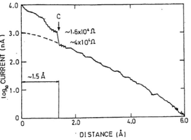
Figure 2.1: Tunneling current (log/) versus distance s for a clean Ir tip and polycrystalline Ag surface at constant bias voltage 20 mV. [Rets. 2 and 24].

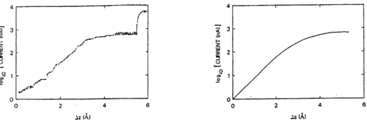
metallic (Ir) tip pressing the Ag surface. By measuring lo g / versus s curve they found important deviation form simple exponential behavior as illustrated in Fig. 2.1. Deviations are seen more clearly in Fig. 2.2 in which selected data are s h o w n . A t small excursions (Az < 3.5 A ) the separation s between the tip and the sample is relatively large, and the curve is typical for tunneling. The apparent barrier height (/»gfr is as high as 3.5-5 eV in STM mode. As the tip approaches towards the surface, the barrier height is reduced resulting in a plateau in log I versus s curve corresponding to a saturation resistance Rs- Lang^^ calculated the resistance plateau using the adatom-on-jellium model for a Na atom tip, and found Rs = ARc where Re = /i/2e^ ~ 12900 D is the constriction resistance^^ associated with a one dimensional conduction channel which connects two reservoirs, and A is a constant (higher than unity^^) depending on the kind of the tip atom.

CHAPTER 2. TRANSPORT IN STM 9

Figure 2.2: Tunneling current (log/) versus excursion A z measured from the starting point where the resistance is 20 Mil (at constant bias voltage 20 mV). Left panel: Experimental result for a clean Ir tip and polycrystalline Ag surface. Right panel: Theoretical result for a Na atom tip. [Refs. 2 and 21].

On further decreasing the separation s, a discontinuous jump occurs in current. Consequent abrupt change in resistance (approximate values given in Fig. 2.1) indicates the onset of quantum point contact. Gimzewski and Möller estimated an initial contact radius, 7’c, of 1.5 A according to the Sharvin lormula assuming <C /e> ^i^d they concluded that initially the contact must be of

CHAPTER 2. TRANSPORT IN STM 10

atomic dimensions. A hysteresis pattern suggesting adhesion occurs between tip and sample was also observed in the experiments with large excursions (A^r > 5

A),

whereas the variation of log I is reversible for A z < 5

A.

In conjunction with these results, Sutton and Pethica^^ demonstrated strong adhesion between clean surfaces (involving inelastic flow) which makes the tip and the sample jump to contact with very small separations (~ 1.5

A

in Fig. 2.1). In this way, discontinuous jump in current is attributed to mechanical instability caused by atomic motion under the influence of adhesive forces. Moreover, in a tight-binding study Ferrer et. al?‘^ argued that the tunneling resistance should saturate at a minimum value of Rs = Rc if no instability would occur at the onset of point contact.

2.2

STM Studies of Graphite

The two forms (hexagonal and rhombohedral) of graphite cannot be isolated and single crystals are difficult to obtain and their size is generally small. For these reasons, polycrystalline pyrographite is usually studied in scanning tunneling microscopy (STM). The most widely used form is highly oriented pyrolitic graphite (HOPG) whose misorientation angle is less than 2 degree.^’ The scan size in a typical STM study is smaller than the grain size (3 — 10 ¡.an) of HOPG,^® hence it provides atomically fiat surfaces of sufficiently large area. Together with that, the easy preparation of HOPG sample (simply by cleaving), and the inertness of the graphite surface towards chemical reactions have made graphite the standard test and calibration sample.

As explained in Sec. 3.1, the carbon atoms in an ideal graphite (0001) surface form honeycomb structure. Three alternating atoms of each hexagon (specified as A sites of the lattice) lie in a different environment than the other three atoms (B sites). While A sites face A sites directly below in the adjacent layer, B sites face the center of the hexagons (H sites). The atomic flatness of large terraces of cleaved graphite was confirmed by STM images in early experiments performed in ultra-high vacuum (UHV) and in air. However, (0001) surface was seen as

CHAPTER 2. TRANSPORT IN STM 11

a triangular lattice, rather than a honeycomb lattice. The spacing between the topographic maxima was found equal to the second-nearest-neighbor distance of graphite. Electronic structure c a l c u l a t i o n s ,l a t e r , showed that B sites exhibit a higher LDOS at Fermi level than A sites; H sites exhibit the lowest. Thus, only B site atoms were expected to be seen as protrusions; A sites should appear as saddle points, and H sites should result depressions. This phenomena is denoted as the site asymmetry. It was found nearly independent of polarity within bias voltage range [—0.2, 0.2] V, and this independence is attributed to atomic force interactions. On the other hand, site-selective imaging^® of A and B sites can be achieved by reversing the bias polarity when the bias voltage is larger than a threshold value (0.5 V).

Bias dependent STM studies yield also important information on the sample electronic structure. Experimentally, the decrease of the corrugation amplitude was observed with increasing bias voltage as, indeed, predicted earlier by theoretical analysis.^' This decrease was noticed only at high voltages if the tip-sample interaction dominates.

The site asymmetry would not be expected to exist for graphene, i.e. a monolayer extracted from graphite. However, triangular arrangement of maxima are seen in STM images of graphene on a P t ( l l l ) surface.^" The Fermi surface of graphene reduces to a point at the edge of the Brillouin zone. Consequence of that is imaging a single state. The nodes of the wave function of this individual state do not depend on the atomic position in the unit cell and lead to large corrugations with the periodicity of the unit cell.^^ In bulk graphite, the Fermi surface is very narrow, but finite because of the weak interlayer interaction, and lifts the nodes of the wave function. Nevertheless, the image is dominated by the same individual state.

In the STM studies of graphite, giant corrugations (up to 8 Â or even more) are often observed in the constant current mode of operation. The corrugation of Ü.8Â was calculated for contours of constant LDOS at Fermi level, which flatten out to 0.2 Â (also determined by helium diffraction data) for the contours of total charge density. While imaging a single state, the nodal structure of the wave

CHAPTER 2. TRANSPORT IN STM 12

f function enhances the corrugation amplitude up to 1 Beyond this value, giant corrugations are attributed to local elastic deformations^® of the surface that are induced by atomic force between the tip and the sample. Such deformations enhance the corrugation due to the electronic density of states. This e.xplanation is also confirmed by experiment: The corrugation amplitude was found smaller than

0.1 A

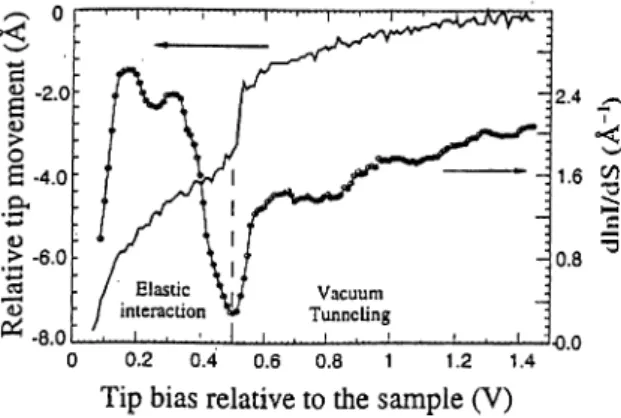
under the condition of free tip-sample mechanical interactions.^®

Figure 2.3: The measurement of the tip movement and d ln J /d s , as a function of the tip bias at a constant tunneling current of 1 nA. [Ref. 26].

Transition to the elastic deformation regime is clarified in Fig. 2.3 by the variation of the decay rate k. At about 0.5 V, the barrier height (f) (which is related

to 2/c = d ln //(/s ) collapses. Nevertheless, it remains finite even at that value of the bias voltage. Below this transition voltage, d l n lj i ls has no relevance to (j) because of elastic deformations which are also indicated by nonlinear variations of the tip movement.

Chapter 3

ATOMISTIC SIMULATIONS

3.1

Atomic Structure of Graphite

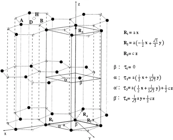
Graphite has a hexagonal lattice structure with lattice constants a and c as defined in Fig. 3.1. It posses a layered structure with honeycomb arrangements of carbon atoms on (basal) planes. The layers are weakly bonded to one another, but also well separated. Experimental values of the nearest neighbor distance (o /\/3 ) and the interlayer spacing (c/2) are respectively 1.42 Â and 3.337 Â at zero te m p e ra tu re ,a n d 1.418 Â and 3.348 Â at room temperature.^^ Since c to a ratio is much greater than the ideal closed-packed value, graphite is far from being hexagonal closed-packed.

Graphite is the most stable allotrope of carbon, except that diamond is more stable at very high pressures. The interatomic distance (1.418 Â) in graphitic plane is shorter than that of diamond (1.54 Â) and reflects the thermodynamical stability. The diamond value is close to the carbon-carbon single bond length (1.55 À), whereas that of graphite is stronger than single bond, but yet it is weaker than double bond (which corresponds to 1.33 Â bond lengtld“'). In this respect, graphite is similar to benzene molecule. Benzene has 1.39 X bond length,^'* and experimental fact^’^ is that all bond lengths in benzene are equal and lie between that of single and double carbon bonds.

Graphite can be in different forms according to the stacking of its basal

CHAPTER 3. ATOMISTIC SIMULATIONS 14

planes. The most common form is the hexagonal (Bernal) graphite with A B A B stacking of layers. In rhombohedral graphite, layer stacking is A B C ABC] the

A A A sequence occurs in first stage intercalates, e.g. alkali metal intercalated

graphite. Intercalation describes the insertion of guest agents between graphite layers with metallic-type bonds. In pseudopotential calculations,^'*’^^ total energy differences were found to be smaller than 0.005 eV per atom among these three forms, showing also the weakness of interlayer interaction. In the weak interlayer interaction the Van der Waals bonding between widely separated graphitic planes has a significant contribution. On the other hand, planar bonds are strong covalent bonds with hybridization of carbon electrons. With this anisotropy in bonding, graphite is highly ordered within layers but stacking sequence may

Ri = a X R,= a ( - i x + :^ y ) Rj= c 2 p : x,= 0 a : X2= a ( { x + ^ y ) a': + P'· '^4=

CHAPTER 3. ATOMISTIC SIMULATIONS 15

be erratic, or can be made erratic e.g. by pyrolizing. This general form is called pyrographite, or pyrolytic graphite.

The Bernal structure has two inequivalent atoms {a', /3' in the planar unitcell drawn in Fig. 3.1) per layer, and layers are staggered so that each a atom has atoms a' directly above and below in adjacent layers whereas ¡3 sees hollow center of corresponding hexagon. ¡3' is on the center of the neighboring hexagon. The structure can also be described as combining two hexagonal lattices of a and f3 atoms. The unitcell is then defined by the primitive vectors R i, R 2, R 3 of these lattices as shown in Fig. 3.1. R 4 is added to represent the surfaces in a more appropriate way. In hexagonal systems, the surfaces are labeled by four indices

(ijkl) corresponding to the vectors Rx, R 2, R 4, R 3. The index along R 4 is

always related to two of others: k = —(i + j). In such a labeling system, the top layer, for instance, is represented by (0001). There are four atoms in the unitcell with the position vectors Ti, T2, T3, T4. In this work, the positions of a and ^ atoms are labeled as A and B sites respectively. The center of hexagon is II site; the mid-point between a and ¡3 atoms is labeled as the bridge D site.

3.2 Interatomic Carbon Potential

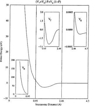
The interatomic potential V used in this work was developed by Nordlund et (to its final form) by combining three distinct potentials:

V(r¡¡) = [Vrira) + + V„(r„)[l - F(r¡¡)], (3.1) where r.ij is the distance between ¿th and j t h atom. The total energy of the atomic system (in a given configuration) E is then expressed as a summation over all atom pairs:

(.3.2)

1

7^ i

in terms of the interatomic interaction energy V(r,j). This description seems to be similar to that of pair potentials, however, there is an important difference due to the implicit many-body interactions in Vt and Vo- Nevertheless, it also

CHAPTER 3. ATOMISTIC SIMULATIONS ₁₆

differs from cluster potentials in that there is no summation over higher-order atom multitudes.

Despite the fact that the potential describes several carbon polytypes reasonably; the combination of three potentials are mainly required for graphite. The main contribution, the Tersoff potential^’’ Vr, gives a good description of covalent bonding, and describes diamond and graphene fairly good. But, unfortunately, its range is so short that the weak interaction between graphite layers is not included. For this reason, Nordlund et. introduced a long-range potential Vg to include bonding between graphite layers. Besides, a repulsive ab

initio potential Vr is included in order to treat the strong repulsion between the atoms when the interatomic distance is very small. This repulsive potential prevents the structure from collapsing.

Tersoff^*^ had gone beyond the conventional two- and three-body potentials in transferability and accuracy by introducing a new family in view of the quantum- mechanical arguments. Mciin observations were the universal binding-energy curve of Rose et and its e.xponential parameterization given by Abell. Rose et have shown that the binding energy versus atomic separation curve can appro.\imately be scaled into a single universal relation for metallic adhesion and the cohesion of bulk metals. This universal form predicts the curve relative to the equilibrium. AbelT^ parameterized the binding energy (within local orbital chemical pseudopotential theory) as Morse-like pair potentials to guarantee the universality. Moreover, he made an interpretation of the Pauling’s bond order

i.e. the strength of the bonding with respect to the bond length, to include the

topologic effects relative to a reference system. These ideas are incorporated in the empirical potential by T ersoff,introducing exponential pair potentials, and realizing the bond order as depending on the local atomic environment. Hence, the potential was designed in the following functional form:

(3.3)

CHAPTER 3. ATOMISTIC SIMULATIONS 17

overlapping atomic wave functions:

fnirij) = A

and an attractive pair potential associated with bonding:

fA{r.i) = - B e - " » ,

(3.4)

(3.5) and a smooth cutoff function f c to shorten the range of the potential for fast computations:

fc{rij) = <

1, R

5 + 1 cos(7T^::^), R < ra < D (3.6)

0, Vij > D

In Eqns. (3.4) and (3.5), parameters A and B restrict the strength of repulsion and attraction respectively, and and determines the range of the corresponding potentials. R in Eqn. (3.6) is the actual range of the complete potential; from R to D the potential goes to zero. Beyond Z), there is no interaction in any pairs.

In Eqn. (3.3), bij is a measure of the bond order. The determination of a satisfactory form of this term is the key point of Tersoff potential. As discussed by AbelE^ and Te r s of f , t he bond order is a monotonically decreasing function of atomic coordination number Z, i.e. the number of neighbors close enough to form bonds. Moreover, as also observed in ab initio calculations,'*^ b{j must grow more rapidly than with decreasing coordination, and saturate at low coordination to give an energy minimum at an intermediate coordination. To satisfy this behavior, Tersoff^** assumed that

6„ = (i + r G ) - ‘'"", (3.7)

where the effective coordination term (ij counts the other bonds of the ¿th atom beside the ij bond:

CHAPTER 3. ATOMISTIC SIMULATIONS 18

The cutoff function f c takes A:th atom (as a bonding neighbor) into account if it is sufficiently close to fth atom. The existence of such a bonding neighbor decreases

bij, and therefore interaction energy of the ij pair is reduced. As a result the ij

bond is weakened. In Eqn. (3.7), the parameters ¡3 and n are introduced to yield a proper generalization of the coordination number. The function g treats the bond-angle forces within the effective coordination term:

6^

(P (P + (ti — cos OijkY ’

where dijk is the angle between two bonds, ij and ik. The parameter u corresponds the cosine of the energetically optimal angle, d determines how sharp the dependence on angle is, and b measures the strength of the angular effect. W ith these, g is constrained to the correct angular coordination within local environment of any atom. The other function e gives yet another cutoff for bonding of neighbors,

(3.10)

4rij,rik) = e

where determines the range of bonding. If the parameter R allows only first- neighbor interaction within a model description, g is effectless unless it equals to /i. In any case, g can be set to equal to g.

The bond order depends upon the local coordination of the fth atom with its neighbors, making the potential more transferable. Transferability, in such a classical model, means the ability of correct description of the interaction between atoms under different local environments. In this model, it is clear that the interaction energy of a pair differs as its surrounding changes. Furthermore, the contributions of a pair of atoms are not equal in a given configuration due to the asymmetry in bond order, i.e. b{j ^ bji, and hence F (r,j) ^ V(vji).

In the present implementation, the first and second nearest neighbors are in the range of Vy, so none are accounted for different layers. In contrast, Vg takes the main contribution from neighboring atoms on adjacent layers, and negligible amount from the ones within the same layer (by the effect of defined below). The two potentials are then of different ranges, and summing up the two does not destroy the description of the relevant potential in its own range. In this way.

CHAPTER 3. ATOMISTIC SIMULATIONS 19

an independent extension of the potential is achieved to give nonzero interlayer forces th at are completely absent in Tersoif potential. Vg is mainly a Morse potential Vm fitted to the experimental force curve^® . However, as mentioned before, a many-body term (f):i is also introduced for interplanar bonding, which simultaneously reduces Vm within a monolayer. Therefore,

0, Tij <i 'I'Mfi

V o i r i j ) = < <í>3ÍGij)VM{rij), rM,o < Tij < r M , i

. 0, nj > r,v/,i

(3.11)

with

Vviirij) = Ko - - I f . (3.12) The reason for the low-end cutoff rM,o is explained above, and the high-end cutoff tm.i is introduced for efficient molecular dynamics simulations,^'^ i.e. for computational purposes. Vc^ is a parameter to adjust the minimum of the

interlayer interaction energy, cq is formally the equilibrium interlayer spacing, and /4 determines the range of the interlayer interaction. In Eqn. (3.11), the many-body term is G',j with the following definitions:

U G i f = (3.13)

(3.14)

Gij = X) <l>i{9ijk)<i>2[f'ik)· k^i.j

W ithout being affected very much by the value of G'ty, the parameter /0 reduces the Morse potential by a few order of magnitude. The effect of ^3 is to reduce high-energy contributions of three first-nearest neighbors. —VcJq is the interaction energy between layers (through a atoms) without three-body modulations which is through the following functions:

h iT it ) = 1 (3.15) i + ( “ i f “ )·'’ 'hiO.it) = 1 (3.16) j 1 ^COS 6ijky^

CHAPTER 3. ATOMISTIC SIMULATIONS 20

4>2 makes the first-neighbors effective in bonding of planes (as long as parameter ro chooses first neighbors within a range determined by /2) whereas (¡>1 prefers the triples with an angle close to the right angle (provided by the value of parameter /1). Therefore, there is a trade-off in between to optimize the effect of the surroundings of atom pairs. Consequently, the planar bonding is basically between the a and a.' atoms of successive layers of graphite. Because the coordination number of graphene, i.e. 3, is subtracted from Gij to tolerance to

/3, ^3 prevents high energy contributions of three nearest-neighbors of an atom when it is binding to adjacent layers.

The third potential Vr in Eqn.3.1 is the repulsion energy of carbon-carbon dimer. It is of the form of numerical data“* * obtained by doing spline interpolation to the results of dense density functional calculations within the local density approximation.^® Vr is smoothly fitted to the Tersoff potential as expressed in

Eqn. (3.1) by using the following Fermi function:

n r i j ) = 1 (3.17) With this fitting the interaction between two atoms which are closer (further) than 77 is effectively determined by Vr (Vt). hj gives the range of transition

from Vr to Vx.

The parameters of the potential were determined by Tersoff^' and Nordlund

et Vt is fitted to the cohesive energies of carbon polytypes, along with lattice constants and bulk modulus of diamond. The results of ab initio calculations“*^ were used when measurements became unavailable. Tersoff determined the parameters R and D somewhat arbitrarily, and set tj equal to zero for simplicity. The parameters in Vq and F are determined by experimental data*®’“**·’ and by fitting of the interplanar energy versus lattice parameter c curve to the experimental one,“*® and by another energy fitting to the diamond-to-graphite transition curve.“*” Nordlund et al. optimized the parameter D, and set 77 ecjual to ¡j.. The final parameters are as follows: 7? = 1.8

A,

= 2.46

A,

/1 = 1.3936 X 10® eV, A = 3.4879

A~\

B = 3.467 x 10'^ eV, fi = 2.2119 k ~ \

CHAPTER 3. ATOMISTIC SIMULATIONS 21

Figure 3.2: The energy oi the carbon dimer. The ranges of Vr, Vt and Vo become clear in the insets. The extension of the range of the Morse potential results a very weak barrier as shown.

d = 4.3484, u = -5.7058 x lO-^, co = 3.348

A,

lo = 0.0456 eV, h = 0.15,

ro = 1.46

A,

k = 0.21

A,

/i = 0.07.

In addition to what is described above, a minor modification of the potential was made in the present study. Owing to the transition data in its construction, the potential is able to choose the right local (tetrahedral) environment rather than the graphitic coordination under the influence of high pressure. However, there is a gap in the case of uniaxial compression between interlayer spacing values 2.46

A

and 2.87

A

as it is well understood from the given parameters that the potential becomes identically zero in this range (without destroying the cpiality of predictions for near-equilibrium properties of graphite). A linear interpolation of Vr and Vo is made from 1.8

A

to 2.87

A

keeping the parameters unchanged. The range of Vo is extended towards that of Vt in this way; the effect of this modification is seen in Fig. 3.2 for carbon-carbon dimer by adding a very weak

CHAPTER 3. ATOMISTIC SIMULATIONS ₂₂

Figui’e 3.3: Total energy versus lattice parameter c. The zero of the energy is set to the equilibrium value at c = 6.696

A.

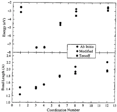
barrier to the potential. As shown in Fig. 3.3, the combination of Vr and Vq results in a flat region near the vicinity of the equilibrium, and the slope gained by the Tersoff potential remains too small in comparison with the experimental curve. The interpolation extends the range in which the interlayer energy curve lies close to the experimental one. The transferability of the potential is not destroyed, and is slightly improved for high-coordinated structures as seen in Fig. 3.4. In addition, the energy versus interatomic distance curves for all carbon poly types mentioned in Fig. 3.4 do not differ significantly from those of the form that was used by Nordlund et near the equilibrium. Finally, the linear interpolation is assumed to be crude in calculating forces, but no instabilities

CHAPTER 3. ATOMISTIC SIMULATIONS ₂₃ -2 3 -_4 _ ti n W -6 -7 - 8 2.4 2.0 ’ 1.8 1.6 o C2 1.4 -1.2 1.0 9 m ♦ H----h H----l· • Ab Initio ♦ Modified ■ Tersoff

t

4 5 6 7 8 9 Coordination Number ■“ I— t H----l· É 10 11 12 13

Figure 3.4: The transferability of the interatomic carbon potential. The values on horizontal axis represents dimer(l), graphite(3), diamond(4), simple cubic(6), body-centered cubic(8), and face-centered cubic(12) structures, in order.

(arising from jumps in force in the range of interpolation) are identified in molecular dynamics simulations. Hence, even though the interpolation made may be regarded as an artificial procedure, the resulting form of the potential is reliable for simulation purposes as much as the previous forms.

Any binding phenomenon corresponds to a (local) minimum in Born- Oppenheimer (BO) potential energy surface, i.e. the configuration energy with respect to atomic degrees of freedom. The potential given above is capable of describing BO surface since the bond order bij follows the variations of BO surface with respect to atomic positions: The attraction of atom pairs is modulated by

bij; the values of bij's depend on the position of the atomic configuration relative

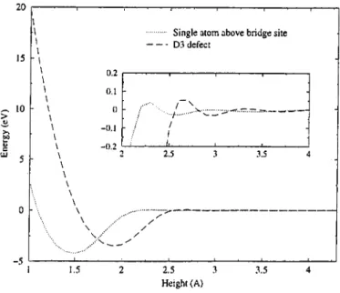
to the extrema of the BO surface. This feature makes the potential favorable for molecular dynamics simulations. As an example, binding of a single carbon atom to (multilayer) graphite is illustrated in Fig. 3.5. When the atom is about

CHAPTER 3. ATOMISTIC SIMULATIONS 24 20 15 10 \ \ \ \ ■ \ \ \ \ \ - \ \ \ 5 0 --5 0.2 0.1 0 -0.1 -0.2

... Single atom above bridge site --- D3 defect 2.5 3 \ ..·· / \ .■_\ ··■ _^/ 3.5 1.5 2.5 3 Height (A) 3.5

Figure 3.5: Binding of a single carbon atom to the graphite lattice.

1.5 Á above D site, binding occurs with an energy of —4.21 eV. If a graphitic plane was present in place of the single atom, there would be strong repulsion as deduced from Fig. 3.3. Thanks to the presence of term, the bond order tends to vanish in the case of a graphitic plane whereas it is nearly unity for the single atom. The other curve in Fig. 3.5 is an additional, e.xample, and is drawn to determine the binding energy of a D3 defect, i.e. a surface defect formed by an atom above D site which lifts two neighboring atoms (a and /3) on the top layer. These three atoms form a vertical ring whose shape is nearly equilateral triangle. The topmost atom and the neighboring a and /? atoms are about 2 Á and 0.4 Á higher than undisturbed lattice, respectively. The distance between a and /3 atoms is approximately 7% longer than the equilibrium value. Nordlund et verified that the D'i defect structure is stable, and suggested that it may be source of hillocks higher than 2 Á observed experimentally. Their ab initio calculation gave a binding energy of —3.3 eV. The interatomic potential yields —3.33 eV at 2 A , however the minimum of energy ( —3.46 eV) is at 1.9 A .

CHAPTER 3. ATOMISTIC SIMULATIONS 25

3.3 Molecular Dynamics Simulations

The formation of an atomic-size contact on the graphite (0001) surface is simulated by using the classical molecular dynamics (MD) method with the empirical potential described in the previous section. In this section, a brief summary of classical MD method is presented, and the results of the simulations are discussed. In the classical MD method, the atomic interactions are modeled by an empirical potential, and Newtonian equations of motion are solved for each atom in the system by a finite difference method which is 7-Value Gear predictor-corrector in this work. The algorithm of the computations is simply as follows:

1. Predict the positions and derivatives at time i -1- t by making a Taylor expansion about time t:

-I- r) = r(¿) -t- rv (i) + ^ r^a(i) -I---,

-f r) = v(f) -|- ra (i) + · · ·, up to sixth order 2. Evaluate forces from the gradient of the interatomic potential energy:

F,· = - V r . F

3. Correct predicted quantities using the Gear corrector coefficients Cq,Ci, r'=(ii) = Cofa“^ - a^],

v ‘^(i) = v ^ ( i ) c j a · ^ — a^], up to sixth order

4. Calculate any variables of interest

The system investigated is a tip-sample system which is represented by two models of different size. The sample is a graphite slab comprising 6 (or 8) layers,

i.e. (0001) planes. Each layer contains 308 (or 448) atoms, making total number

of sample atoms 2016 (or 3584). The hard and sharp metal tip (such as W) is represented by a robust diamond tip; it comprises 13 (111) diamond planes, and

CHAPTER 3. ATOMISTIC SIMULATIONS 26

contains 167 atoms. The apex of the tip has a single atom, and the higher layers contains 3,3,6,6,10,10,15,15,21,21,28,28 atoms, in order. Periodic boundary conditions are imposed to the slab only in the lateral directions (.t and y), and the tip is not periodic at all. The system is divided into static and dynamic regions in an artificial way; all atoms belonging to the tip and to the lowest two layers of the sample are kept fixed in the integration procedure. The remaining atoms are treated dynamically. The tem perature is rescaled to 2 K at every two steps to avoid possible divergences in the kinetic energy of moving atoms. The time step was r = 1 x 10“ ^® in accordance with high-order Gear algorithm.'*®

Initially, the tip is at s = 2.5

A

above the sample, and then it is pushed down towards the sample in the course of the simulation. The strategy of pushing the tip towards the sample is as follows: The sample is first equilibrated in 500

4850 -> >> W) <u c W -4950 o 0. -5050 -5150 5000 15000 25000 35000 45000 Number of MD steps 55000

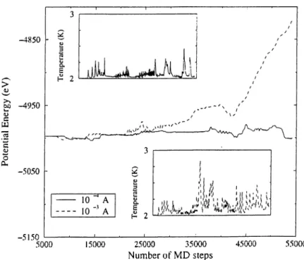
Figure 3.6: Variation of the potential energy and convergence of the tem perature during test simulations. The tip and sample are in highly repulsive interaction. 5000 relaxation steps were needed to equilibrate the system fully before the push of the tip starts.

CHAPTER 3. ATOMISTIC SIMULATIONS 27

relaxation steps before the start of pushing. Since the interaction is very weak between the sample and the tip, that amount of time is found to be sufficient. The equilibration is terminated when the fluctuations in the total energy settled down. Then the tip is pushed at a rate of 1 x 10““*

A

per time step for 500 steps, and then the system is relaxed during the next 500 steps. The velocity of the tip (100 m / s ) is small enough to allow the system reequlibrate between successive instabilities if any occur. At the end of each 500 relaxation steps total energy fluctuations settle down, and the temperature converges to 2 K.

Some test calculations are performed to find a reliable and fast strategy of pushing. The rate of pushing should be large enough to avoid the long simulation times. On the other hand, it should be sufficiently small in order to fully eciuilibrate the system. Simulations with two values of the pushing rate ( l x 10“^

A

and 1 X 10“^

A)

are compared in Fig. 3.6. The smaller value seems to be more appropriate for stable simulations.

3.3.1 Results and Discussion

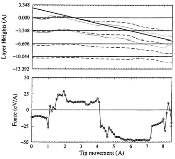
The tip is located at various positions (A, B and H sites) in the .Ti/-plane, and it is pushed towards the surface at constant x and y. Relatively large relaxations occur initially in the course of pushing the tip. Near the contact the tip compresses the slab, and eventually punctures the topmost layer. These variations are more clearly seen in Fig. 3.7, where the solid lines represent the undisturbed layers; the dashed lines show the average changes in layer heights; the dotted lines show the variations of the positions of the atoms within close proximity of the tip apex of the first and second layers. The heavy line represents the tip position. In the lower panel, the variation of the force on sharp tip is shown. Figs. 3.8 and 3.9 include the same information for H and A sites, respectively.

At the beginning, the tip is 2.5

A

above the surface where there is attractive tip-sample forces in all three cases. When it is pushed down by 1

A

above B site repulsive forces increase. The slab is then compressed by dominant repulsive forces until the downwards displacement of the tip reaches to 4

A.

At this value

CHAPTER 3. ATOMISTIC SIMULATIONS 28

.s? ‘C

X

Tip movement (A)

Figure 3.7: The variation of the layer heights and the force with the movement of the tip above B site.

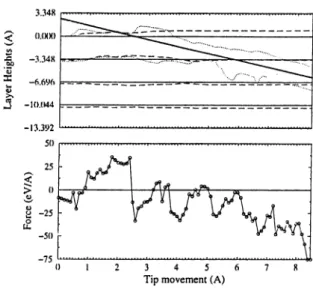
3.348 0.000 : ■a -3.348 s ^ -6.696 -10.044 -13.392

Figure 3.8: The variation of the layer heights and the force with the movement of the tip above H site.

CHAPTER 3. ATOMISTIC SIMULATIONS 29

-10.()44

-13.392

Figure 3.9: The variation of the layer heights and the force with the movement of the tip above A site.

sudden transition to attractive interaction is attributed to the puncture of the topmost layer.

It is exciting to observe that the force characteristics for the B (H) site converts into that for the H (B) site in the course of the push. This is what one normally expects from the atomic structure since B and H sites change alternatively in successive graphitic planes, and gives further evidence for successive puncturing of layers.

Fig. 3.9 explains local deformations more clearly. In Figs. 3.10, 3.11, 3.12 and 3.13 some important snap-shots of the simulations are shown for the tip above A site. In this case puncturing is rather fast, and the local environment of the apex follows the tip. The tip enlarges the puncture and eventually breaks the surface into flakes as shown in 3D pictures.

CHAPTER 3. ATOMISTIC SIMULATIONS ₃₀

Figure 3.10: The puncture of the first layer by the tip above A site.

Figure 3.11: Disloccition-inducecl crashes in the first layer. Behind is the tip whose apex is between the first and second layers.

CHAPTER 3. ATOMISTIC SIMULATIONS 31

Figure 3.12: The first layer has already been broken into flakes before the tip punctures the second layer.

Chapter 4

SCF PSEUDOPOTENTIAL

CALCULATIONS

4.1

Total Energy Calculations

The self-consistent field (SCF) calculations are performed in momentum space within local density approximation(LDA) to examine the effect of the tip applying a uniaxial strain to the graphite surface. The ionic potential of carbon is replaced by the nonlocal, norm-conserving“*® pseudopotentials taken from the table of Bachelet et. The components of the ionic potential are shown in Fig. 4.1. The exchange-correlation energy is approximated by Ceperley-Alder (CA) form.®* A plane wave basis set (whose size is determined by the kinetic energy cutoff |k -f G p ) is used within the framework of momentum space formalism“^ of the density functional theory®® (DFT). The kinetic energy cutoff is taken to be 37 that corresponds to approximately 900 plane waves for equilibrium structure. The number of plane waves ranges from 550 to 1030 for distorted structures. The irreducible wedge of the Brillouin zone is sampled by 48 points generated from a uniform 6 x 6 x 10 mesh in reciprocal space. The SCF cycles are iterated until the rms deviation of the self-consistent potential is smaller than 1 X 10~' Ry during each calculation. To test the convergence on the plane wave expansion, some calculations are performed with various kinetic energy

CHAPTER 4. SCF PSEUDOPOTENTIAL CALCULATIONS ₃₃

Figure 4.1: The pseudopotential components Kore, AVq“’'', AVi‘‘ AK'"'^ for carbon. The subscript denotes the angular momentum quantum number /. The Coulomb potential is added for comparison. In notation of Ref. -50, is decomposed into a long-range Coulomb part Kore, and a short range /-dependent pseudopotential part A K ‘°"·

cutoffs (33,37,39, and 45 Ry). The k-point sampling is also tested by the meshes 6 X 6 X 6,6 X 6 X 10, and 6 x 6 x 12. The change in the total energy is smaller than 0.5% in each case. The accuracy of a standard LDA calculation is expected to be appro.ximately 1%,®‘* thus, the calculations in this chapter are considered convenient and sufficiently accurate for the purpose of the present study.

4.2 Band Structure of Graphite

The ground state configuration of carbon is Is^ 2s^ 2p^. Is electrons are core electrons, and the remaining four are regarded as valance electrons. Bonding in two natural allotropes of carbon i.e., graphite and diamond, is mainly covalent with different hybridization of atomic orbitals. Graphite monolayer,

CHAPTER 4. SCF PSEUDOPOTENTIAL CALCULATIONS ₃₄

Gi =

G ,= _{2 aTJ >}— 4 - K

Gj= — k,3 Q 7.

Figure 4.2: Brillouin zone of graphite and the irreducible wedge

{■s,px,py) hybridize to form localized sp"^ bonds, and form a bonds between two

nearest carbon atom in the same plane. The p, orbitals perpendicular to the layer remain nonhybridized and form delocalized tt bonds. The residual interlayer bonding is basically due to the overlap of orbitals and partly due to long-ranged Van der Waals forces, i.e. dipole-dipole interaction originated from correlated motion of electrons in different planes,®® and is very weak in comparison with the intralayer bonding. This binding anisotropy is reflected to the structure of graphite whereas diamond has isotropic structure as a result of sp^ hybridization.

In the band structure of graphene, sp^ bonds form three occupied a bands. Near the Fermi level lie a pair of tt bands (one nearly full, the other nearly empty) derived from p, orbitals. The graphite unit cell consists of two weakly bonded unit cells of the graphene as explained in Sec. 3.1. Thus, the band structure of graphite can be approximated by weakly splitting each graphene band into two as shown below.

The band structure of graphite is plotted along the symmetry lines which define the irreducible wedge of the Brillouin zone (BZ). The first BZ of graphite is drawn in Fig. 4.2. The full zone is reduced to 1/24 due to the symmetry properties of graphite. The high-symmetry points are as labeled on the irreducible part, and their group-theoretical properties®® are given in Table 4.1.

CHAPTER 4. SCF PSEUDOPOTENTIAL CALCULATIONS 35

Symbol N The group of k Order of the group

(0,0,0) Deh 24 (0_,0_,1₎ A Deh 24 (0,0, Ç.) C6v 12 (1/3,1,0) K _Dzh 12 (1/3,1,1) H _Dzh 12 (1/2,1/2,0) M _Dzh (1/2,1/2,1) _Dzh (1/3, l,ç .) C-·3v (1/2,1/2, g.) U a2v {qx,qx,0) A c.2v (qx, qx, 1) Q a2v (<Zx/2,(?x/2,0) C2v i q x / 2 , q x / 2 , l ) R C_2v (qy/0, %, 0) T 2v iqyl3,qy,l) a2v

Table 4.1: The special points and the lines of symmetry in the Brillouin zone of the hexagonal lattice. The wave vector k is represented by Q according to

[K,ky,L·] = [{2Tr/a)Qx,(27r/y/3a)Qy,{27r/c)Qz], and 0 < < 1, 1/2 < q,j < I, and 0 < < 1. N denotes the number of vectors in the star of k.

The calculated band structure of Bernal graphite is illustrated in Fig. 4.3 for the equilibrium value of c. It is clear that a bands separate into low-energy (bonding, cr) and high-energy (antibonding, cr*) states with a gap in between. The first unoccupied cr* band is approximately 6 eV^ above the highest occupied cr band at F point where the gap takes its minimum value. In contrast to that 7T bands are closer to each other and as well as closer to the Fermi level. For this reason, various phenomena relevant to relatively low energy transfer such as the electronic conduction are mainly characterized by ~ bands near Fermi le\'el produced by p.-type orbitals.

The cr-band gap do not allow a bands to contribute to the density of states in the vicinity of the Fermi level. In contrast, the tt and ~* bands have nonzero contribution, and moreover, tt and tt* bands join at the K point, causing the band gap to disappear. Thus, graphite is a semimetal, i.e. a material with vanishing gap between valance and conductance bands.