Gas Generator Pressure Control in Throttleable
Ducted Rockets: A classical and adaptive control
approach
Anil Alan
∗and Yildiray Yildiz
†Bilkent University, Cankaya, Ankara, 06800, Turkey
Umit Poyraz
‡and Utku Olgun
§Roketsan Missiles Inc., Elmadag, Ankara, 06780, Turkey
This paper describes the control of gas generator pressure in throttleable ducted rockets using nonlinear adaptive control as well as classical control approaches. Simulation results using the full nonlinear and time-varying dynamics of the gas generator are reported in both classical controller and adaptive controller cases. “Closed-loop Reference Model” structure is used together with the adaptive controller to improve transient response. Controllers are simulated to test their robustness by introducing uncertinities, disturbances and noise to the system. Cold Air Test Plant (CATP) is used as the test facility to compare the controllers and validate the results from simulations. Moreover, damping effect of CRM to oscillations in adaptive controller case is observed in CATP tests.
Keywords: throttleable ducted rockets, pressure control, adaptive control, classical control, cold air test plant, closed-loop reference model
I.
Introduction
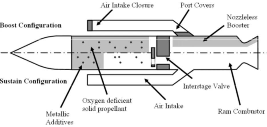
A Throttleable Ducted Rocket (TDR) is basically a ramjet engine where the fuel is provided via the
burning of an oxidizer deficient propellant.1 What makes these rockets “throttleable” is the ability to adjust
the thrust by varying the mass flow rate of the fuel.2 Fig. 12shows the basic components of a TDR. Nozzleless
booster is used at the beginning of the operation to make the rocket reach to a high enough Mach Number that can support the ram effect. During this initial stage, the solid propellant in the gas generator (GG) is ignited with the help of hot booster gases and after a transition phase, when the rocket reaches to a certain Mach Number, the rocket is propelled solely with the combustion of the fuel, delivered from the GG, at the ram combustor. The mass flow rate of fuel delivered to the ram combustor is adjusted using a valve between the GG and ram combustor. The focus of this paper is the control of GG pressure by manipulating the valve position in order to achieve a required GG pressure profile that is dictated by the thrust need. This thrust need is determined by the outer loop thrust controllers (or mach controllers) whose job is to calculate the required thrust to realize the mission requirements. The outer loop controllers will be the subject of future research and therefore will not be considered in this study.
The control of the pressure either in GG of TDRs or in conventional solid rocket propellants has been
studied by many researchers both in academia and in industry. One of the early studies is conducted
by Thomaier3 where GG pressure is approximated as a first order lag dynamics and a gain scheduled
proportional(P)-proportional and integral(PI) controller cascade is used as the controller, together with
sev-eral logic units. Thomas and Ostrander4 use open loop control to control the GG pressure for an air turbo
rocket engine, where necessary throat opening schedule for desired pressure values are carefully determined
∗Graduate student, Mechanical Engineering Department.
†Assistant Professor, Mechanical Engineering Department.
‡Senior Propulsion Systems Design Engineer, Propulsion Systems.
§Senior Mechanical Design Engineer, Propulsion Systems.
1 of 13
Downloaded by BILKENT UNIVERSITY on October 5, 2017 | http://arc.aiaa.org | DOI: 10.2514/6.2015-4236
51st AIAA/SAE/ASEE Joint Propulsion Conference July 27-29, 2015, Orlando, FL
AIAA 2015-4236 AIAA Propulsion and Energy Forum
using previous motor test data. Bergmans and Myers,5 researchers from the same company, at the time, showed results basically using the same setup and controllers, where the emphasis was on the valve
devel-opment. Sreenatha and Bhardwaj6 use a PI controller where the gains are scheduled based on the control
volume in the GG. Another linear controller design using PI gains is performed by Davis and Gerard7where
they use the controller as a variable thrust solid propulsion controller. Pinto and Kurth8use a gain scheduled
PI controller together with a feedforward (FF) term, which increases the speed of the system by calculating
the required steady state throttle area given a desired GG pressure. An interesting study by Chang et al9
describes the design of a linear controller that addresses the nonminimum phase behaviour of the thrust dynamics by using a combination of the GG pressure and Ram Combuster pressure as the feedback variable.
Another linear control approach is adopted by Niu et al10 where a PI controller is designed using static
output feedback (SOF). Same authors implement the SOF controller in another study11 where they
intro-duce a “switching controller” which chooses the best control input among two different controllers during
the operation. Bergmans and Salvo12 linearize GG pressure dynamics around a nominal operating pressure
and a nominal throat area and a linear controller, details of which are not provided, is designed using this linearized model. The linear controller dynamics are updated periodically based on the estimation of the free volume inside the GG, using the fact that the linearized model pole location is inversely proportional to this free volume.
Another approach in gas generator pressure control is funnel control,13which is a proportional controller
with a varying gain. The gain is adjusted in such a way that the error of the closed loop system remains inside a predefined boundary (or funnel, hence the name). One practical disadvantage of funnel control
is that although the error stays inside a funnel, it may not converge to zero.14 This disadvantage can be
alleviated by combining the funnel control with a PI controller.15 There are some restrictions on the plant
dynamics for which funnel control is to be implemented. One of these restrictions is that the plant must be minimum phase meaning that the zero dynamics should be stable. Another restriction is that the plant must have relative degree 1, however it is possible to eliminate this restriction by introducing an auxiliary output
variable and obtaining an auxiliary system dynamics.16, 17 In the control of GG pressure, funnel control is
used successfully by Bauer et al18for flight performance evaluation using adjustable simulation models and
also in ground and flight tests by Besser and Kurth.19
Finally, Lee et al20 proposes an adaptive sliding mode control approach to compensate for the
uncer-tainties and nonlinearities in the pressure dynamics in a solid propulsion system. Successful simulations are provided without any experimental results.
In this paper, the control of GG pressure is investigated both from adaptive control and classical control
perspectives. The contribution of the paper are as follows: 1) A model reference adaptive controller21 is
implemented for the GG pressure control, both in simulation and experiments. 2) A PI controller is designed based on predefined system specifications and using a step by step approach minimizing the trial and error phase for the selection of control parameters. 3) Both of these control approaches are compared in simulation as well as in experimental setup.
The paper is organized as follows: In Section II, the model of the GG pressure dynamics is provided. In Section III, the design of adaptive and classical controllers are described. In Section IV, simulation results are provided. In Section V, experimental setup is described. In Section VI, a conclusion is given.
II.
System Model
As mentioned above, the inner control loop, namely the gas generator (GG) pressure control loop, is the main focus of this paper. In general, a high fidelity model of a given system facilitates the controller design by reducing the uncertainty, to the extent possible. In the case of GG pressure control, the model of the system is the mathematical relationship, described by a nonlinear differential equation, between the valve
opening (input) and the GG pressure (output). This relationship is studied by many groups2, 3, 8–10, 18, 19and
a brief summary of the results are provided below.
A. GG Pressure Dynamics
Consider the GG section in Fig 1. The mass flow rate, into the GG is given as ˙
mb= Arρ (1)
Figure 1: Throttleable ducted rocket components.2
where ˙mb is the mass flow rate of the burnt propellant into the GG and A, r and ρ are the burning area,
burning rate and the density of the propellant, respectively. Burning rate r is a function of the GG pressure and is determined as
r = aPgn (2)
where the constants a and n are functions of the temperature and pressure in the GG and are generally
found empirically. Pg is the GG pressure. Defining c1≡ Aaρ and combining (1) and (2), it is obtained that
˙
mb= c1Pgn. (3)
Assuming choked flow in the throat (or interstage valve), mass flow rate out of the GG can be given as
˙ mout= Ath Pg √ T r γ R( γ + 1 2 ) −γ+1 2γ−2 (4)
where Athis the throat opening, R is the gas constant, T is the temperature in the GG and γ is the specific
heat ratio. Defining c2≡√1TpRγ(γ+12 )− γ+1
2γ−2, (4) can be rewritten as
˙
mout= c2AthPg. (5)
Assuming isothermal conditions, i.e. constant temperature, using the ideal gas law, its derivative and utilizing (1) and (4) it is obtained that
PgVg = mgRT ˙ PgVg+ PgV˙g = ˙mgRT = ( ˙mb− ˙mout)RT ˙ PgVg+ PgV˙g = (c1Pgn− AthPgc2)RT ˙ Pg = −Pg ˙ Vg Vg + Pgnc1RT Vg − Pg Athc2RT Vg . (6)
It is noted that ˙Vg can be determined as ˙Vg= rA = aPgnA and therefore (6) can be rewritten as ˙ Pg= −Pgn+1 aA Vg + Pgn c1RT Vg − Pg c2RT Vg Ath (7)
Defining c3≡ aA, c4≡ c1RT and c5= c2RT , (7) can be rewritten as ˙ Pg= −c3 Pn+1 g Vg + c4 Pn g Vg − c5 Pg Vg Ath. (8)
Equation (8) provides the mathematical relationship, in a compact way, between the variable that is
desired to be controlled, which is the GG pressure Pg and the control input, which is the throttle opening
Ath. It is noted that this relationship is not only nonlinear but also time-varying, due to the changing control
volume Vginside the GG. It is known that nonlinearity and time-varying dynamics make the controller design
a challenging task. One approach can be linearizing the system dynamics around an equilibrium point by
assuming a constant Vg. This procedure is explained below.
Making the following definitions
c6≡ c3 Vg c7≡ c4 Vg c8≡ c5 Vg (9) equation (8) can be rewritten as
˙
Pg= −c6Pgn+1+ c7Pgn− c8PgAth. (10)
Linearizing around an equilibrium GG pressure Pg0 and the corresponding throttle opening Ath0, it is
obtained that ˙
Pg= − c6Pg0n+1+ c7Pg0n − c8Pg0Ath0− (n + 1)c6Pg0n(Pg− Pg0) + nc7Pg0n−1(Pg− Pg0)
− c8Ath0(Pg− Pg0) − c8Pg0(Ath− Ath0). (11)
With the following definitions
c9≡ (n + 1)c6Pg0n c10≡ nc7Pg0n−1 c11≡ c8Ath0 c12≡ c8Pg0
c13≡ c10− c9− c11 (12)
equation (11) can be written compactly as
∆ ˙Pg= c13∆Pg− c12∆Ath. (13)
B. Overall Plant Model with Actuator Dynamics
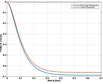
The nonlinear relationship between the throat area of nozzle and chamber pressure was studied in previous subsection. In order to achieve a desired pressure profile, pressure controller needs to define a desired throat area value for the nozzle. Desired throat area requirement is fulfilled by an actuator at the throat. Dynamics of the actuator is assumed to have first order dynamics with a time constant τ . Together with this actuator dynamics, overall plant transfer function is determined as:
G(s) = Kol
as2+ bs + c (14)
Using the system parameters and assumed actuator time constant, open loop response of the linearized system to a step input is given in Figure 2. It is noted that Fig. 2 also contains the response of nonlinear GG dynamics given in eq. 8 along with assumed actuator dynamics to the same step input. As seen from the figure, linear and nonlinear dynamics show reasonable agreement.
III.
Controller Design
As shown in Section II, the relationship between the control input of the system (valve opening) and the controlled variable (GG pressure) is described by a first order, nonlinear, nonautonomous differential
Figure 2: Step response of linearized and nonlinear GG with same actuator dynamics
equation (8). In addition, due to many simplifying assumptions such as constant control volume, constant temperature and ideal gas behavior together with ignoring the effects of the particles in the propellant, the derived dynamics contains considerable uncertainty. One way to cope with the uncertainty is using adaptive control, which updates its parameters online based on the the change of system signals and tracking error. Another approach is designing linear controllers that are robust enough to take care of uncertainties. There are also robust nonlinear control approaches that can be used if the bounds on the uncertainties are known. In this section, the design of two of these approaches, namely adaptive control and robust linear controllers are explained. For both controllers, output feedback method is used, because it is assumed that the only measurable state of the system is pressure of gas generator by pressure sensors. For adaptive control design case, it is assumed that actuator dynamics are faster than the gas generator dynamics, which makes gas generator dynamics dominant in overall system. Hence, nonlinear adaptive controller is designed according to the gas generator dynamics and effect of actuator dynamics is assumed to be compansated by the adaptation in adaptive controller.
A. Nonlinear Adaptive Controller
Consider the following nonlinear plant which represents the nonlinear GG dynamics. ˙
x = a1f1(x) + a2f2(x) + bu(t)x(t) (15)
where x(t) = yp(t) is the pressure of GG, f1(x) = xn and f2(x) = xn+1 are nonlinear functions of x, n
is the constant burning exponential of solid booster and u is the outlet throat area. With the assumption
of constant GG volume, coefficients a1, a2 and b are found to be constant and dependent on the physical
parameters of the system. A nonlinear controller could be assumed as u(t) = −k1f1(x) − k2f2(x) − k3x(t) + k4r(t)
x(t) (16)
where r(t) is the bounded reference input to the closed loop system and k1, k2, k3 and k4 are controller
parameters. When (16) is embedded into (15), closed loop system becomes, ˙
x = (a1− bk1)f1(x) + (a2− bk2)f2(x) − bk3x + bk4r. (17)
Stable reference model desired to be followed is given as ˙
xm= amxm+ bmr. (18)
Assuming that the system coefficients are known, desired control parameters can be obtained as, k1∗=a1 b k2∗=a2 b k∗3 =−am b k∗4= bm b . (19)
At nominal conditions, controller (16) with controller parameters given in (19) would manipulate the system (15) towards (18) without any problem. However, this controller would not be robust enough to compansate the uncertinities in system parameters. In order to compansate the uncertainties, controller parameters are updated online, where the adaptive laws are given as
˙ k1= f1(x)e1(t)sign(b)Γ1 ˙ k2= f2(x)e1(t)sign(b)Γ2 ˙ k3= x(t)e1(t)sign(b)Γ3 ˙ k4= −r(t)e1(t)sign(b)Γ4 (20)
where e1(t) = x(t) − xm(t) is the error between plant output and reference model output, sign(b) represents
the directional relationship between the input and output of the nonlinear plant and Γi for i = 1, 2, 3, 4 are
positive constants to define the adaptation rates of controller parameters. Defining ˆki(t) = ki(t) − k∗i for i = 1, 2, 3, 4 and finding the time derivative of error signal as ˙e1= ame1− b ˆk1f1(x) − b ˆk2f2(x) − b ˆk3x + b ˆk4r by substracting eq. (18) from eq. (17), the stability of the system can be proved by using standard Lyapunov Stability Analysis utilizing a Lyapunov function candidate given as
V (e, k1, k2, k3, k4) = e21 2 + ˆ k12 2 + ˆ k22 2 + ˆ k23 2 + ˆ k24 2 . (21)
B. Closed-loop Reference Model (CRM)
In adaptive control, a high adaptation rate increases the speed of the system response in the expense of increased transient oscillations. If the rates are kept low, then the oscillations tend to dissapear but tracking performance of controller reduces as well. In order to tackle this problem without sacrificing the performance,
Closed-loop Reference Model (CRM)22structure is introduced to the nonlinear adaptive controller. In CRM,
tracking error between the plant response and reference model response is fed back to reference model, which
in turn reduces the osciallations in the system response inspite of relatively high adaptation rates.22
To implement CRM, the original reference model (18) is modified as ˙
xm= amxm+ bmr − l(x − xm) (22)
where xm(t) is the reference model state and x(t) is the plant state and r(t) is the bounded reference signal.
For am, l < 0, reference model and error dynamics are stable.
C. Linear Control Design
To obtain a satisfactory response, the following specifications for the closed loop system are determined: a) zero steady state error, b) a bandwidth of 3rad/sec and a phase margin of 85 degrees. (It is noted that in the adaptive controller design these specifications are imposed in the reference model (18).)
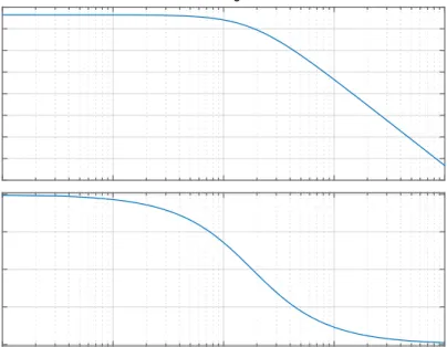
Bode plot of the plant is given in Fig. 3. To satisfy the requirements of bandwidth, steady state error and the phase margin, a PI controller with a zero at s = −10 with corresponding P and I gains is chosen. The frequency response of the overall system together with the designed PI controller is given in Fig. 4. It is seen from the figure that all the specifications are satisfied.
Magnitude (dB) -80 -70 -60 -50 -40 -30 -20 -10 0 10-1 100 101 102 103 Phase (deg) -180 -135 -90 -45 0 Bode Diagram Frequency (rad/s)
Figure 3: Bode plot of uncompansated system
Magnitude (dB) -90 -80 -70 -60 -50 -40 -30 -20 -10 0 10 100 101 102 103 Phase (deg) -180 -150 -120 -90 Bode Diagram Frequency (rad/s)
Figure 4: Bode plot of system with PI controller
IV.
Simulation Results
In this section, adaptive and classical controllers designed in previous sections are tested in the simulation environment. Plant model, consisting of nonlinear GG model together with actuator dynamics is first created in the software environment. Then, PI controller and nonlinear adaptive controller with CRM structure is added to the system with suitable gains predetermined in the design phase.
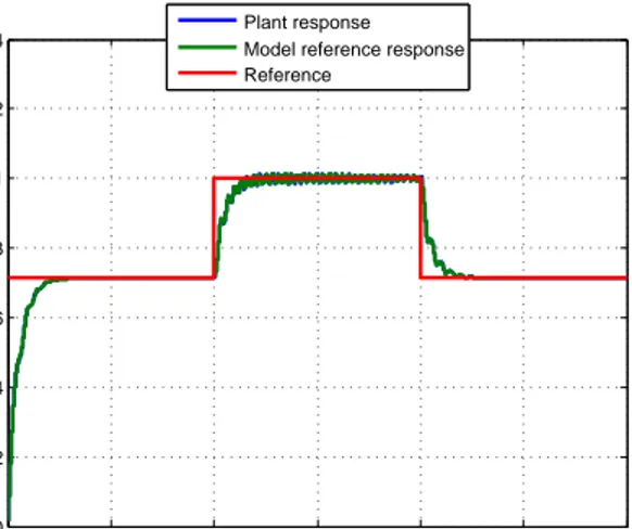
Before a comparison with a proportional-integral (PI) controller, the adaptive controller is simulated to show the effect of the CRM structure on the system performance for different gains. As seen in Figs. 5-10 tuning the CRM gain to obtain an oscillation free system is fairly straightforward.
After obtaining a reasonable response for the adaptive controller with a suitable CRM gain, the controllers
0 1 2 3 4 5 6 0 0.2 0.4 0.6 0.8 1 1.2 1.4 time [sec] Pressure
Time Series Plot: Plant response Model reference response Reference
Figure 5: Plant response with l = −500
time [sec] 0 1 2 3 4 5 6 Throat Area 0 0.1 0.2 0.3 0.4 0.5 0.6 0.7 0.8 0.9
1 Time Series Plot:
U(t)
Figure 6: Controller response with l = −500
0 1 2 3 4 5 6 0 0.2 0.4 0.6 0.8 1 1.2 1.4 time [sec] Pressure
Time Series Plot: Plant response Model reference response Reference
Figure 7: Plant response with l = −1000
time [sec] 0 1 2 3 4 5 6 Throat Area 0 0.1 0.2 0.3 0.4 0.5 0.6 0.7 0.8 0.9
1 Time Series Plot:
U(t)
Figure 8: Controller response with l = −1000
are tested for the ideal case, where no uncertainy or noise is present in the system. As seen in Figs. 11 and 12, both PI and adaptive controller show acceptable performance for the ideal case. In real life applications, the effects such as noise, nozzle throat eroding due to excessive heat and imperfections in solid propellant are expected, which drag the system away from ideal conditions. Besides, assumptions made while getting the mathematical model of the GG (ideal and isotropic gas assumption) do not hold. Hence, the designed controllers need to be robust enough to compansate the uncertainties due to these phenomena. To test the robustness of the controllers, uncertainties and noise are added to the plant dynamics and the controllers are tested againts these conditions. One of the possible scenarios during GG operation is that the mass flow rate into the control volume, created by the burning of the solid propellant, could be less than modeled. Physically, this uncertinity could be caused by a couple of cases such as voids in solid propellant, metallic additives in gas medium and nonuniform burn at the end of the propellant. This uncertinity is introduced to simulations by decreasing the mass flow rate by 20%. Apart from this uncertinity, white noise is added to the system representing the noise from pressure transducers. As seen in Fig. 13-16, both the designed PI controller and the adaptive controller show promising results in the presence of uncertainties and noise.
0 1 2 3 4 5 6 0 0.2 0.4 0.6 0.8 1 1.2 1.4 time [sec] Pressure
Time Series Plot:Plant response Model reference response Reference
Figure 9: Plant response with l = −10000
time [sec] 0 1 2 3 4 5 6 Throat Area 0 0.1 0.2 0.3 0.4 0.5 0.6 0.7 0.8 0.9
1 Time Series Plot:
U(t)
Figure 10: Controller response with l = −10000
time [sec] 0 1 2 3 4 5 6 Pressure 0.6 0.65 0.7 0.75 0.8 0.85 0.9 0.95 1 1.05
1.1 Time Series Plot:
Reference Plant response
Figure 11: Plant response with PI controller in ideal conditions. time [sec] 0 1 2 3 4 5 6 Pressure 0.6 0.65 0.7 0.75 0.8 0.85 0.9 0.95 1 1.05
1.1 Time Series Plot:
Plant response Model reference response reference
Figure 12: Plant response with nonlinear adaptive controller in ideal conditions
V.
Experiments
A. Experimental Setup
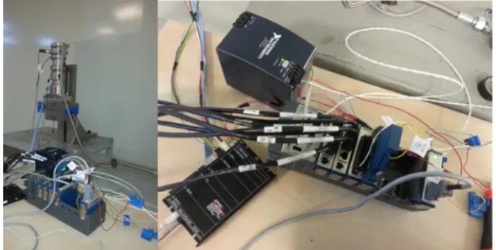
Fig. 17 depicts the test setup in ROKETSAN Inc. The test setup mainly consists of gaseous nitrogen source, regulator, piping, solenoid valve, mass flow meter, pressure transducers, variable throat mechanism and its control hardware. A nitrogen bundle has been used as the source in order to get rid of the variable upper stream conditions which affect the test results by reducing the mass flow rate and total pressure. To be able to measure the fluid properties and test quantities at different locations and commanding the control signals to the actuator of the variable throat mechanism, National Instrument cards and LabView is used as shown in Fig. 18.
Mass flow rate from nitrogen bundles to the system is kept constant taking advantage of a pressure regulator. At the valve outlet of the system, a pintle-throat mechanism is used to manipulate the throat area. Pintle is controlled by a BLDC motor whose rotation is converted into linear motion by a spindle mechanism. There are maximum and minimum throat area limitations dependent on the valve and pintle geometry. These values are tested and corresponding pressure values are used to determine the operating range of the system. Plant output is read by pressure sensors in the control volume. Noise from these sensors
0 1 2 3 4 5 6 0.5 0.6 0.7 0.8 0.9 1 1.1 time [sec] Pressure
Time Series Plot:Reference Plant response
Figure 13: Plant response with PI controller in the presence of uncertinity and noise.
0 1 2 3 4 5 6 0.5 0.6 0.7 0.8 0.9 1 1.1 time [sec] Pressure
Time Series Plot:Plant response Model reference response Reference
Figure 14: Plant response with nonlinear adaptive controller in the presence of uncertinity and noise.
0 1 2 3 4 5 6 0 0.05 0.1 0.15 0.2 0.25 time [sec] T h ro a t A re a
Time Series Plot:
U(t)
Figure 15: Controller response of PI controller in the presence of uncertinity and noise.
0 1 2 3 4 5 6 0 0.05 0.1 0.15 0.2 0.25 time [sec] T h ro a t A re a
Time Series Plot:
U(t)
Figure 16: Controller response of nonlinear adaptive controller in the presence of uncertinity and noise.
are suppressed by a regular low-pass filter.
Volume is constant in Cold Air Testing Plant (CATP) while it is time-dependent in GG. Moreover, mass flow rate to the control volume can be kept constant in CATP, however it is a function of pressure in GG. Other than these major differences, GG and CATP has similar characteristics with CATP having less risk and cost. Hence, CATP provides a suitable alternative to test various pressure control approaches for gas generators.
B. Experimental Results
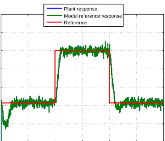
Employing the Cold Air Testing Plant detailed in Section A, tests are conducted to compare the performances of the PI controller and the adaptive controller. The results are reported in Figs. 19-24. It is noted that data is normalized.
As seen from the figures, both PI controller and adaptive controller was able to manipulate system to track the reference input. However, in the PI controller case, output signal is oscillatory and it takes a considerable amount of time to reach its steady state value. Accordingly, PI controller signal is also oscillatory. Transient response can be improved by decreasing the controller gains but this may cause undesirably slow response
Figure 17: Test setup Figure 18: Control Hardware. Actutor and DAQ Unit.
dynamics. It is seen from the figures that when the adaptive controller is implemented, the response of the system is smoother together with a smooth control signal. The performance of the adaptive controller can further be improved by introducing robustfying terms to the algorithm, which will be addressed in future studies. 0 10 20 30 40 50 60 70 80 0 0.1 0.2 0.3 0.4 0.5 0.6 0.7 0.8 0.9 1 Time [sec] Pressure Plant Response Reference
Figure 19: Response of CATP with PI controller
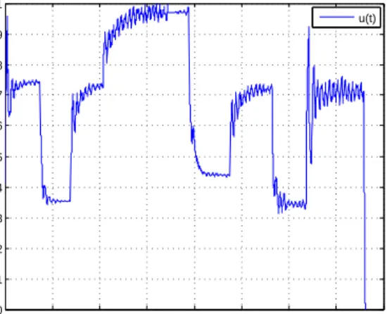
0 10 20 30 40 50 60 70 80 0 0.1 0.2 0.3 0.4 0.5 0.6 0.7 0.8 0.9 1 Time [sec] Throat Area u(t)
Figure 20: PI controller output
VI.
Conclusion
In this paper, adaptive and classical control approaches are investigated for the control of gas generator (GG) pressure in throttleable ducted rockets (TDR). These investigations are carried out both in simulation and experiments. In the adaptive controller case, a nonlinear adaptive controller with a model reference tracking is used to compensate the differences between designed optimal conditions and real application
cases with uncertinities and disturbances. In the linear controller case, the robustness to uncertainties
are realized by imposing careful closed loop control specifications. For the adaptive case, a novel Closed-loop Reference Model approach is added to controller in order to suppress the oscillations caused by high adaptation gains. In simulations, it is shown that both PI controller and nonlinear adaptive controller have satisfactory results for uncertinity scenarios and disturbances. Then, adaptive and classical controller are implemented in Cold Air Testing Plant to reproduce the same results as in simulations. Also, effect of CRM structure to oscillations are shown in simulations and tests.
With a couple of improvements in test setup, more accurate results could be taken. In that case,
0 10 20 30 40 50 60 70 80 0.3 0.4 0.5 0.6 0.7 0.8 0.9 1 Time [sec] Pressure Plant Response Reference
Figure 21: Response of CATP manipulated by adap-tive controller with CRM (l = −25)
0 10 20 30 40 50 60 70 80 0 0.1 0.2 0.3 0.4 0.5 0.6 0.7 0.8 0.9 1 Throat Area Time [sec] u(t)
Figure 22: Adaptive controller output for l = −25
0 10 20 30 40 50 60 70 80 90 0.4 0.5 0.6 0.7 0.8 0.9 1 Time [sec] Pressure Plant Response Reference
Figure 23: Response of CATP manipulated by adap-tive controller with CRM (l = −100)
0 10 20 30 40 50 60 70 80 90 0 0.1 0.2 0.3 0.4 0.5 0.6 0.7 0.8 0.9 1 Time [sec] Throat Area u(t)
Figure 24: Adaptive controller output for l = −100
robustifying modifications in adaptive control algorithm such as sigma modification and projection could be implemented to improve the results. Moreover, different control approaches such as Funnel control or sliding mode control methods could be tested in CATP.
Both PI controller and adaptive controller shows promising preliminary results in CATP as a pressure controller of gas generator as expected from simulations. As next step, these controller algorithms will be tested in Hot Air Testing Plant and will be prepared for gas generator tests.
References
1P. W. Hewitt, Numerical Modeling of a Ducted Rocket Combustor With Experimental Validation. PhD thesis, Virginia
Polytechnic Institute and State University, 2008.
2C. Bauer, F. Davenne, N. Hopfe, and G. Kurthy, “Modeling of a throttleable ducted rocket propulsion system,” in Proc.
AIAA/ASME/ASEE Joint Propulsion Conference & Exhibit, (San Diego, California), pp. 1–15, 2011.
3D. Thomaier, “Speed control of a missile with throttleable ducted rocket propulsion,” in Proc. Advances in Air-Launched
Weapon Guidance and Control 15 p (SEE N88-19553 12-15), 1987.
4M. Ostrander and M. Thomas, “Air turbo-rocket solid propellant development and testing,” in Proc.
AIAA/ASME/SAE/ASEE 33th Joint Propulsion Conference and Exhibit, 1997.
5J. L. Bergmans and R. I. Myers, “Throttle valves for air tur-bo-rocket engine control,” in Proc. AIAA/ASME/SAE/ASEE
33th Joint Propulsion Conference and Exhibit, 1997.
6A. G. Sreeriatha and N. Bhardwaj, “Mach number control-ler for a flight vehicle with ramjet propulsion,” in Proc.
AIAA/ASME/SAE/ASEE 35th Joint Propulsion Conference and Exhibit, no. AIAA 99-294, (Los Angeles, CA), 1999.
7C. A. Davis and A. B. Gerards, “Variable thrust solid propulsion control using labview,” in Proc.
AIAA/ASME/SAE/ASEE 39th Joint Propulsion Conference and Exhibit, no. AIAA 2003-5241, (Huntsville, Alabama), 2003.
8P. Pinto and G. Kurth, “Robust propulsion control in all flight stages of a throtteable ducted rocket,” in Proc.
AIAA/ASME/ASEE Joint Propulsion Conference & Exhibit, no. AIAA-2011-5611, (San Diego, California), pp. 1–12, 2011.
9J. Chang, B. Li, W. Bao, W. Niu, and D. Yu, “Thrust control system design of ducted rockets,” Acta Astronautica,
vol. 69, no. 1, pp. 86–95, 2011.
10W. Y. Niu, W. Bao, J. Chang, T. Cui, , and D. R. Yu, “Control system design and experiment of needle-type gas
regulating system for ducted rocket,” Journal of Aerospace Engineering, vol. 224, no. 5, pp. 563–573, 2010.
11W. Bao, B. Li, J. Chang, W. Niu, and D. Yu, “Switching control of thrust regulation and inlet buzz protection for ducted
rocket,” Acta Astronautica, vol. 67, no. 7, pp. 764–773, 2010.
12J. L. Bergmans and R. D. Salvo, “Solid rocket motor control: theoretical motivation and experimental demonstration,”
in Proc. AIAA/ASME/SAE/ASEE 39th Joint Propulsion Conference and Exhibit, pp. 20–23, 2003.
13A. Ilchmann, E. P. Ryan, and C. J. Sangwin, “Tracking with prescribed transient behaviour,” ESAIM: Control,
Optimi-sation and Calculus of Variations, vol. 7, pp. 471–493, 2002.
14H. Schuster, C. Westermaier, and D. Schroder, “Non-identifier-based adaptive control for a mechatronic system achieving
stability and steady state accuracy,” in Proc. IEEE International Conference on Control Applications, pp. 1819–1824, 2006.
15A. Ilchmann and H. Schuster, “Pi-funnel control for two mass systems,” IEEE Transactions on Automatic Control,
vol. 54, no. 4, pp. 918–923, 2009.
16C. M. Hackl and D. Schroder, “Funnel-control for nonlinear multi-mass flexible systems,” in Proc. IEEE Annual
Con-ference on Industrial Electronics, pp. 4707–4712, 2006.
17C. M. Hackl, C. Endisch, and D. Schroder, “Funnel-control in robotics: An introduction,” in Proc. 16th Mediterranean
Conference on Control and Automation, pp. 913–919, 2008.
18C. Bauer, N. Hopfe, P. Caldas-Pinto, F. Davenne, and G. Kurth, “Advanced flight performance evaluation methods
of supersonic air- breathing propulsion system by a highly integrated model based approach,” in Proc. RTO-MP-AVT-208, pp. 1–14, 2012.
19H.-L. Besser and G. Kurth, “Meteor - european air dominance missile powered by high energy throttleable ducted rocket,”
in Proc. RTO-MP-AVT-208, pp. 1–17, 2012.
20W. Lee, Y. Eun, H. Bang, and H. Lee, “Efficient thrust distribution with adaptive pressure control for multinozzle solid
propulsion system,” Journal of Propulsion and Power, vol. 29, no. 6, pp. 1410–1419, 2013.
21K. S. Narendra and A. M. Annaswamy, Stable adaptive systems. New York: Dover Publications, 2005.
22T. E. Gibson, A. M. Annaswamy, and E. Lavretsky, “Adaptive systems with closed-loop reference models: Stability,
robustness and transient performance,” arXiv preprint, no. 1201.4897, 2012.
![Figure 11: Plant response with PI controller in ideal conditions. time [sec]0123 4 5 6Pressure0.60.650.70.750.80.850.90.9511.05](https://thumb-eu.123doks.com/thumbv2/9libnet/5762411.116611/9.918.516.816.431.668/figure-plant-response-with-controller-ideal-conditions-pressure.webp)