Analysis of sectoral index returns in Turkey with Capm and Treynor and Mazuy models at the pre-, during and post-crisis periods

(1)

ISTANBUL BILGI UNIVERSITY INSTITUTE OF SOCIAL SCIENCES

FINANCIAL ECONOMICS MASTER’S DEGREE PROGRAM

ANALYSIS OF SECTORAL INDEX RETURNS IN TURKEY WITH CAPM AND TREYNOR AND MAZUY MODELS AT THE PRE-, DURING AND

POST-CRISIS PERIODS

Sinem BENLİ 115624013

Assoc. Prof. Serda Selin ÖZTÜRK ISTANBUL

(2)

ISTANBUL BILGI UNIVERSITY INSTITUTE OF SOCIAL SCIENCES

FINANCIAL ECONOMICS MASTER’S DEGREE PROGRAM

ANALYSIS OF SECTORAL INDEX RETURNS IN TURKEY WITH CAPM AND TREYNOR AND MAZUY MODELS AT THE PRE-, DURING AND

POST-CRISIS PERIODS

Sinem BENLİ 115624013

Assoc. Prof. Serda Selin ÖZTÜRK ISTANBUL

(3)

(4)

iii

ACKNOWLEDGMENTS

I would like to express my special thanks to my dissertation advisor Assoc. Prof. Serda Selin Öztürk for the her guidance and answering all of my questions patiently. I really appreciate all her help.

Also, I wish to express my sincere thanks to my colleagues for their support and cooperation. Especially, I feel gratitude to my managers, Oya Töre Bircan, Fuat Kırıkcı, and Belgin Demirci since they provide me with the opportunity to attend all of my classes.

Moreover, I would like to grateful to my parents, Ergün and Hakime Benli, and my sister, Mehtap Benli Akyüz for their tolerance and support during my life.

Lastly, I would like to thank to my friend Okan Turan for his positive outlook and motivation.

(5)

iv

TABLE OF CONTENTS

Page

ACKNOWLEDGMENTS ... iii

ABBREVIATIONS ... vii

LIST OF FIGURES ... viii

LIST OF TABLES ... ix

ABSTRACT ... xi

ÖZET ... xii

INTRODUCTION ... 1

1.1.BASICS OF INDICES ... 1

1.2. 2008 GLOBAL ECONOMIC CRISIS AND EFFECTS ON TURKEY... 1

PART 2: LITERATURE REVIEW ... 4

2.1. LITERATURE WORK ON CAPITAL ASSET PRICING MODEL ... 4

2.2. LITERATURE WORK ON TREYNOR AND MAZUY MARKET TIMING MODEL ... 7

PART 3 : METHODOLOGY ... 9

3.1. TRADITIONAL PORTFOLIO THEORY ... 10

3.2. MODERN PORTFOLIO THEORY ... 10

3.2.1. Systematic Risk ... 12

3.2.2. Unsystematic Risk... 12

3.3. CAPITAL MARKET THEORY ... 14

3.4. CAPITAL ASSET PRICING MODEL ... 16

3.4.1. Market Risk Premium ... 17

3.4.2 Beta ... 17

3.4.3. Security Market Line ... 18

3.5. TREYNOR AND MAZUY MARKET TIMING MODEL ... 20

3.6. THE MODEL ... 22

PART 4: DATA ... 24

PART 5: RESULTS ... 27

5.1. RESULTS FOR BIST BANK (XBANK) INDEX: ... 27

5.2. RESULTS FOR BIST BASIC METAL (XMANA) INDEX: ... 28

5.3. RESULTS FOR BIST INFORMATION TECHNOLOGY (XBLSM) INDEX: ... 30

(6)

v

5.5. RESULTS FOR BIST FINANCIALS (XUMAL) INDEX: ... 32

5.6. RESULTS FOR BIST REAL ESTATE INVESTMENT TRUST (XGMYO) INDEX: ... 33

5.7. RESULTS FOR BIST SERVICES (XUHIZ) INDEX: ... 34

5.8. RESULTS FOR BIST HOLDING AND INVESTMENT (XUHOLD) INDEX: .. 36

5.9. RESULTS FOR BIST CHEMICAL, PETROL AND PLASTIC (XKMYA) INDEX: ... 37

5.10. RESULTS FOR BIST LEASING AND FACTORING (XFINK) INDEX: ... 38

5.11. RESULTS FOR BIST NON-METAL MINING PRODUCT (XTAST) INDEX:39 5.12. RESULTS FOR BIST METAL PRODUCTS MACHINERY (XMESY) INDEX: ... 40

5.13. RESULTS FOR BIST TRANSPORTATION (XULAS) INDEX: ... 42

5.14. RESULTS FOR BIST INDUSTRIAL (XUSIN) INDEX: ... 43

5.15. RESULTS FOR BIST INSURANCE (XSGRT) INDEX: ... 44

5.16. RESULTS FOR BIST SPORTS (XSPOR) INDEX: ... 45

5.17. RESULTS FOR BIST TECHNOLOGY (XUTEK) INDEX: ... 46

5.18. RESULTS FOR BIST TEXTILE (XUTEKS) INDEX: ... 48

5.19. RESULTS FOR BIST TELECOMMUNICATION (XILTM) INDEX: ... 49

5.20. RESULTS FOR BIST WHOLESALE AND RETAIL TRADE (XTCRT) INDEX: ... 50

5.21. RESULTS FOR BIST TOURISM (XTRZM) INDEX: ... 51

5.22. RESULTS FOR BIST WOOD, PAPER PRINTING (XKAGT) INDEX: ... 52

5.23. RESULTS FOR BIST FOOD BEVERAGE (XGIDA) INDEX: ... 54

PART 6: CONCLUSION ... 56 REFERENCES ... 60 APPENDIX ... 62 APPENDIX 1: XBANK ... 62 APPENDIX 2: XBLSM ... 63 APPENDIX 3: XELKT ... 64 APPENDIX 4: XFINK ... 65 APPENDIX 5: XGIDA ... 66 APPENDIX 6: XGMYO ... 67 APPENDIX 7: XHOLD ... 68 APPENDIX 8: XILTM ... 69

(7)

vi APPENDIX 9: XKAGT ... 70 APPENDIX 10: XKMYA ... 71 APPENDIX 11: XMANA ... 72 APPENDIX 12: XMESY ... 73 APPENDIX 13: XSGRT ... 74 APPENDIX 14: XSPOR ... 75 APPENDIX 15: XTAST ... 76 APPENDIX 16: XTCRT ... 77 APPENDIX 17: XTRZM ... 78 APPENDIX 18: XUHIZ ... 79 APPENDIX 19: XULAS ... 80 APPENDIX 20: XUMAL ... 81 APPENDIX 21: XUSIN ... 82 APPENDIX 22: XUTEK ... 83 APPENDIX 23: XUTEKS ... 84

(8)

vii

ABBREVIATIONS

CAPM : Capital Asset Pricing Model REIT: A real estate investment trust GDP: Gross Domestic Product SML: Security Market Line CML: Capital Market Line SMB: Small Minus Big HML: High Minus Low

(9)

viii

LIST OF FIGURES

Page

Figure 1.1: GDP (current US$) ... 3

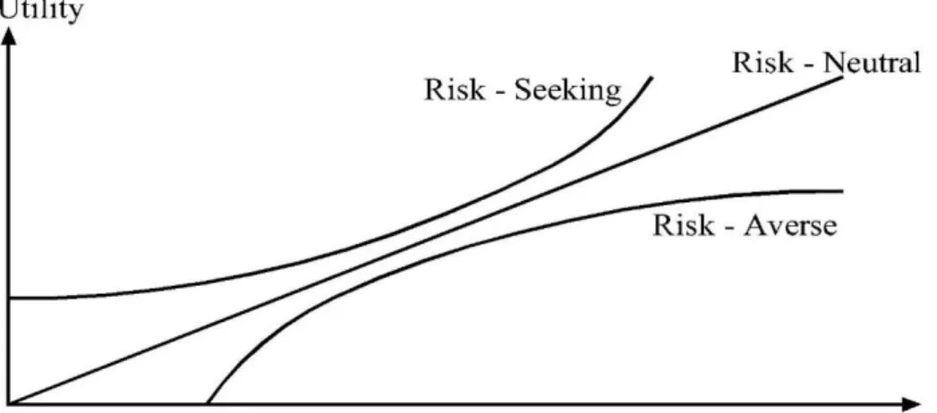
Figure 3.1: Risk Behaviour with utility function ... 9

Figure 3.2: Systematic risk and Unsystematic Risk ... 11

Figure 3.3: Efficient Frontier ... 13

Figure 3.4: Capital Market Line ... 15

Figure 3.5. Security Market Line ... 19

Figure 3.6. Characteristic Line for the fund which able to outguess the market better than average. ... 20

(10)

ix

LIST OF TABLES

Page

Table 1.1 GDP growth rate and Unemployment rate for Turkish Economy ... 2

Table 4.1. Sectoral Index Lists used in the experiment with ticker symbols ... 25

Table 5.1. CAPM and Treynor&Mazuy Regression results for XBANK ... 28

Table 5.2. Market-timing regression coefficient results for XBANK ... 28

Table 5.3. CAPM and Treynor&Mazuy Regression results for XMANA ... 29

Table 5.4. Market-timing regression coefficient results for XMANA ... 29

Table 5.5. CAPM and Treynor&Mazuy Regression results for XBLSM ... 30

Table 5.6. Market-timing regression coefficient results for XBLSM ... 30

Table 5.7. CAPM and Treynor&Mazuy Regression results for XELKT ... 31

Table 5.8. Market-timing regression coefficient results for XELKT ... 31

Table 5.9. CAPM and Treynor&Mazuy Regression results for XUMAL ... 32

Table 5.10. Market-timing regression coefficient results for XUMAL ... 33

Table 5.11. CAPM and Treynor&Mazuy Regression results for XGMYO ... 34

Table 5.12 Market-timing regression coefficient results for XGMYO ... 34

Table 5.13. CAPM and Treynor&Mazuy Regression results for XUHIZ ... 35

Table 5.14. Market-timing regression coefficient results for XUHIZ ... 35

Table 5.15. CAPM and Treynor&Mazuy Regression results for XUHOLD ... 36

Table 5.16 Market-timing regression coefficient results for XHOLD ... 37

Table 5.17. CAPM and Treynor&Mazuy Regression results for XKMYA ... 37

Table 5.18. Market-timing regression coefficient results for XKMYA... 38

Table 5.19. CAPM and Treynor&Mazuy Regression results for XFINK ... 39

Table 5.20. Market-timing regression coefficient results for XFINK ... 39

Table 5.21 CAPM and Treynor&Mazuy Regression results for XTAST ... 40

Table 5.22. Market-timing regression coefficient results for XTAST ... 40

Table 5.23. CAPM and Treynor&Mazuy Regression results for XMESY ... 41

Table 5.24 Market-timing regression coefficient results for XMESY ... 41

Table 5.25. CAPM and Treynor&Mazuy Regression results for XULAS ... 42

Table 5.26. Market-timing regression coefficient results for XULAS ... 43

Table 5.27. CAPM and Treynor&Mazuy Regression results for XUSIN ... 43

Table 5.28. Market-timing regression coefficient results for XUSIN ... 44

(11)

x

Table 5.30. Market-timing regression coefficient results for XSGRT ... 45

Table 5.31 CAPM and Treynor&Mazuy Regression results for XSPORT ... 46

Table 5.32 Market-timing regression coefficient results for XSPORT ... 46

Table 5.33 CAPM and Treynor&Mazuy Regression results for XUTEK ... 47

Table 5.34 Market-timing regression coefficient results for XUTEK ... 47

Table 5.35 CAPM and Treynor&Mazuy Regression results for XUTEKS ... 48

Table 5.36 Market-timing regression coefficient results for XTEKS ... 49

Table 5.37 CAPM and Treynor&Mazuy Regression results for XILTM ... 49

Table 5.38 Market-timing regression coefficient results for XILTM ... 50

Table 5.39. CAPM and Treynor&Mazuy Regression results for XTCRT ... 51

Table 5.40 Market-timing regression coefficient results for XTCRT ... 51

Table 5.41. CAPM and Treynor&Mazuy Regression results for XTRZM ... 52

Table 5.42 Market-timing regression coefficient results for XTRZM ... 52

Table 5.43 CAPM and Treynor&Mazuy Regression results for XKAGT ... 53

Table 5.44 Market-timing regression coefficient results for XKAGT ... 53

Table 5.45 CAPM and Treynor&Mazuy Regression results for XGIDA ... 54

Table 5.46 Market-timing regression coefficient results for XGIDA ... 55

Table 6.1. Mean value of the coefficient in terms of periods and models ... 56

Table 6.2 Number of Beta, which is above one in terms of model and periods. ... 57

Table 6.3. Number of Alpha, which is not significant at any given levels. ... 58

Table 6.4. Average value of Alpha, which are significant at given levels... 58

Table 6.5 Number of insignificant Treynor and Mazuy Estimation ... 59

(12)

xi ABSTRACT

Analysis of Sectoral Index Returns in Turkey with CAPM and Treynor and Mazuy Models at the Pre-, During and Post-Crisis Periods

The Economic Crisis in 2008 has the negative effect on Turkish Economy as both developed and developing countries. To evaluate the effect of the crisis, and also to provide a broad view of the economy, twenty-three sectoral indices at BIST were analyzed. In this dissertation, two main points were considered while analyzing the performance of the indices. First, each of indices riskiness indicators called Beta were estimated with both Capital Asset Pricing Model (CAPM) and Treynor and Mazuy Quadratic Model, and all results analyzed in terms of how they differ according to the models and periods. Additionally, abnormal return coefficient (α) estimations were included the analyzing. Secondly, the indices’ market-timing ability was calculated with the quadratic term at Treynor and Mazuy Market Timing Model. After all regression estimation, the average beta values indicate that the sectoral indices are riskier than the market at the crisis period for Treynor and Mazuy Model, while they seem less risky than the market for CAPM. Also, abnormal return estimations provide that the indices generally create less return relative to their risk. The other important point is that the gamma values estimated with Treynor and Mazuy Unconditional Model were mainly found insignificant at the pre-crisis and post-crisis period; on the other hand, the 60% of the results found significant at the crisis period, and it implies that the indices have market timing-ability either positive or negative.

Key Words: CAPM; Market-Timing; Abnormal-Return; Systematic Risk; Sectoral Indices

(13)

xii ÖZET

Sektör Endeklerinin Finansal Varlıkları Fiyatlama Modeli ve Trenor & Mazuy Piyasa Zamanlaması Modeliyle Kriz Öncesi, Sonrası ve Kriz Döneminde Analiz Edilmesi

2008 Ekonomi Krizi gelişmiş ve gelişmekte olan piyasalarda olduğu gibi Türkiye üzerinde de negatif etkilere neden olmuştur. Bu çalışmada krizin Türkiye’deki etkilerini ölçümlemek için Borsa İstanbul’da yayınlanan yirmi üç sektör endeksi analize dahil edilmiştir. Çalışmada temel olarak iki bakış açısı benimsenmiştir. İlk olarak, her bir sektör endeksinin riskinin kriz öncesi, sonrasında ve kriz döneminde nasıl farklılaştığı Finansal Varlıkları Fiyatları Modeli ve Treynor& Mazuy Piyasa Zamanlaması Modeli’nden elde edilen beta katsayıları ile yorumlanmıştır. Buna ek olarak ise bu dönemlerde yaşanan anormal getiri sonuçları her iki regresyondan elde edilen alfa katsayısı ile çalışmaya dahil edilmiştir. Sonrasında ise yatırımcıların bu dönemlerdeki zamanlama yeteneğinin ölçümlenmesi için yine Treynor&Mazuy Piyasa Zamanlaması Modeline başvurulmuş ve bu modelden gelen gama değerleri dönemler özelinde incelenmiştir. Yapılan çalışmalar sonucunda Treynor and Mazuy’den gelen ortalama beta değerleri sektör endeklerinin kriz döneminde piyasaya göre daha fazla riskli olduğu sonucu çıkarken, Finansal Varlıkları Fiyatlama Modeli sonuçlarına göre ise sektör endekslerinin riskinin piyasa riskinin altında kaldığı gözlemlenmiştir. Bunlara ek olarak, endekslerin anormal getirilerinin genelde negatif yönlü olduğu tespit edilmiştir. Sektörlerin piyasa zamanlama kabiliyetine baktığımızda ise Treynor& Mazuy Model sonucunun genel olarak anlamlı çıkmadığı, sadece kriz döneminde anlamlılık düzeyinin %60 seviyesine geldiği, yani yatırımcıların kriz döneminde pozitif yada negatif zamanlama yeteneğine sahip olduğu gözlemlenmiştir.

Anahtar Kelimeler: Sistematik Risk; Beta; FVFM; Anormal Getiri; Piyasa Zamanlaması

(14)

1

INTRODUCTION

PART 1:

1.1.BASICS OF INDICES

Indexes are the indicators which serve general outlook of the market thanks to including price, costs, production, and weighting details. Firstly, the portfolio of the indices are decided, and the weighting is calculated according to the indicators’ price. Investors uses the indicies when they calculting their porfolios’ movement over time. In this way, the investors can track the changes in the market. Especially, the stock indices are widely used in finance. Indices are not only gives general outlook of the special market, but also they are able to be used in derivative products or funds as an instrument. In this study, I concentrate on the twenty-three sectoral indexes calculated by Borsa Istanbul. The aim of the selection of sectoral indices is that provide general vision of Turkish Economy during both crisis and non-crisis period. In this way, there would be better vision of the sectors.

1.2. 2008 GLOBAL ECONOMIC CRISIS AND EFFECTS ON TURKEY

The economic crisis arise second half of 2007 in America, then it was spread all over the world and turn into Global Economic Crise due to the triggering effect of the capital globalization. There are four main connected reasons why the crisis happen. First, interest rate in America was considerably low since 2000 because of the fact that the government plan to encourage citizens to buy houses with mortgage credit. These credits generally offer 2 year fixed rate, after that it was turned to floating rate. Since the interest rates low, many low-income people started to buy house with mortgage credit. Hence, house prices increase because of the boost in demand. In 2006, Fed decided to hike interest rate. Later, low-income people failure to pay their mortgage credit and house market

(15)

2

entered in recession period. Second reason is securizitation. Since the banks would like to get rid of credit risk they issued debt securities which shows its future earnings as a colleteral. This securities are named collateralized debt obligation (CDOs). These securities were structured financial instruments, which purchase and collect financial assets, and they weighted according to their riskiness. In this way, the banks plan to get rid of risk and share with others. Unfortunately, these securities risk weighting was spoiled because people are

Table 1.1 GDP growth rate and Unemployment rate for Turkish Economy 2007 2008 2009 2010 2011 2012 2013

GDP growth (annual %)

5.0 0.8 -4.7 8.5 11.1 4.8 8.5

Unemployment, total (% of total labor force)

(national estimate)

8.9 9.7 12.6 10.7 8.8 8.1 8.7

Created from: World Development Indicators Country:Turkey

not able to pay their mortgage credit back. At this point, other important reason is occured. Credit rating institions did not downgraded credit rating of this securities. People continued to use derivative products based on these securities. Credit rating institutions were able to downgrade these products rating when the crisis start. This causes the market condition were not early detected by investors and the government. Last but not least problem was transperency. This problem is related to prior reason. Banks and investment companies were not aware of their open position because complicated derivative products effects were hard to be detected. Risk management calculation were not effective. Lastly, many financial institutions, which were known as a too big to fail, were collapsed like Lehman Brothers.

(16)

3 Figure 1.1: GDP (current US$)

(World Development Indicators, 2018)

Though the crisis began in America, it spreaded all over the world within the triggering effect of globalization. Since as in the case of many devoloping countries, Turkey experience shrinking by 4,7 also unemployment rate hike by 12,6 in 2009. Non-performing loan percentage rise to above 4,5% Even so, the effects of the crisis was not be devastating compared to the other economies, because of the precauitions which were taken after the 2001 crisis helped the banking and finance sector to stay strong. On the other hand, the reel economy is affected by lack of hot-money flow, hardship in finding external borrowing, increasing credit-cost and decrease in the foreign trade volume. So, the worsening of the macro indicators is mainly due to problem in the reel economy rather than finance sector. (Ertuğrul, İpek, & Çolak).

(17)

4

PART 2: LITERATURE REVIEW

There are many research made to test investors selectivity skill, evaluating risk and performance in Finance. All of the these experiment generally accepted to start with Markowitz Optimal Portfolio Theory, then it was evaluated by Jack Treynor (1961-1962), William Sharpe (1964), John Linter(1965) and John Mossin (1966) as Capital Asset Pricing Model. Also, one of the other important performance indicator market timing study was carried out by Treynor and Mazuy (1966). They argued whether the investors could forecast the market fluctiation by quadretic term. Though there are many different approach to evaluate performance of the investors or markets performance, I focused mainly these theories. In this section, I try to give overview of the latest work and different approaches which tested these theories in different environment.

2.1. LITERATURE WORK ON CAPITAL ASSET PRICING MODEL

(Çelik, 2013) tested the stability of the sectoral indices betas in Turkish Stock Market during crisis period (2007-2009). She analyzed the stability of the betas by recursive and rolling regression analysis. The finding shows that the beta values don’t have strong characteristic, they are time-variying rather than constant. Also, finding implies that the constant beta might cause the overestimation or underestimation.

The sensitivity of to Market Index and Non-systematic Risk Measurement of Sector Indices in Borsa Istanbul is the paper evaluating performance of CAPM under crisis environment (2010-2012). This paper assume the market index as BIST100 (XU100) and used monthly return of the sectoral indices. They find that some sector indices are more aggreesive than others. They are banking, sport and tranportation; whereas some of sectors are less risky like information technology and trade. (Kaderli, Petek, Doğaner, & Babayiğit, 2013)

(18)

5

(Baillie & Cho, 2016) analyzed the relationship between the euro and other floating currencies’ excess returns on bond market. Also, they consider that there are relationship with euro-dollar and the US and European equity market . They tested these assumption during the crisis period with the respect of International CAPM approach (I-CAPM). With the help of these approach, they evaluate the effect of the US excess equity return on Eurozone equity market. Also, they used the kernel weighted-time varying model to asses the effect of the time on structural parameters and risk-premium terms.Their study concluded that there are significantly relationship between the US and European equity markets and the euro-dollar exchange rate.

(Tuna & Ender, 2013) evaluated the performance of systematic risk indicator beta by Downside Beta (D-CAPM) and traditional Beta on Istanbul Stock Exchange, and made comparison of the estimation power of the expected return for the period 1991-2009. D-CAPM approach take into account only the negative deviations while calculating the beta coefficient called downside, while traditional CAPM don’t consider. The results imply that the D-CAPM approach estimate 1,5% more expected return than traditional method. For these reason, they stated that the D-CAPM is better approach than the traditional CAPM for the applied period.

(Pettengill, Sundaram, & Mathur, 1995) The study focus on the relationship between returns and beta predicted by Sharpe-Linter-Black Model which uses expected return rather than realized return. It is assumed that there are always postive relationship between expected return and beta, but it is conditional relationship if the test realized return and market excess return. The experiments made for the period between 1926-1990. The data set diveded into two group: up market and down market. The results indicates that the beta which measure of systematic risk constant with all period and sub-period. Moreover, positive trade-off between beta and return relation consistent with the later theory. They concluded that beta should continued to be used as a market risk measure.

(19)

6

Another model is adjusted the US T-bill rate by Turkish and US inflation rate difference and used market index as BIST100. The study used beta of the twenty portfolio, which includes 10 stocks for the period between 1995-2004. They used two approach to validiy of the CAPM in Turkey: Fama&MacBeth(1973) and Pettengill et all (1995). For first approach, results indicates that there is no signigificant relationship between beta coefficient and historical risk premiums of the selected portfolios. Second, the strong beta -risk premium relationship were discovered: high-beta stocks have higher positive risk premiums when the market is up, and higher negative risk premiums when the market is down. (Gürsoy & Rejepova, 2007)

(Çoşkun, Selcuk-Kestel, & Yılmaz, 2017) The study based on Turkish REITs to ensure suggestion for the efficientt porffolio management for maximizing their return. The paper was used two model: CAPM and Fama-French three-factor model. The results illustrate that the most of T-REITs have defensive character for CAPM model. Fama-French result shows that the model increase its power of being market indicator. SML-HML approach improves the power of coefficient by taking into consideration the market’s extrem fluctuation.

(Huang & Cheng, 2005) The paper analyzed the regularity of the time-varying betas and Sharpe-Linter CAPM model while adding structural changes in betas. The experimental periods includes 930 monthly observations from July 1926 to December 2003. According to the findings, the most of the break dates same with each others, which implies that there should be at least one structural break. Also, the betas are changing over time with the model, while single model assume they can’t change. The other important point is that Linter hypothesis that expected value of the intercept is zero, but it is accepted by some regimes, while others rejected.

(F.Brune, Li, Kritzman, Myrgen, & Page, 2008) The paper offer new approach for pricing stocks and market integration, and provide calculation of beta on

(20)

7

securities in the developed and the emerging markets. They create a value-weighted index from their sample portfolio to serve as a market index. The study includes 61 portfolio made by several indices, and tested 14.371 securities all over the world. Their finding support that the selection of the market portfolio is more important in the emerging markets than the developed markets. Also, the model claims that the emerging markets have downward trend according to their evel of integration.

2.2. LITERATURE WORK ON TREYNOR AND MAZUY MARKET TIMING MODEL

(Şahin, 2017) analyzed the market-timing ability of the 7 number of BIST30 index fund managers between January, 2005 and December, 2015 by using Treynor-Mazuy, Henriksson Merton and Jensen-Alfa models. The results show that none of fund manager have significant market-timing ability according to the result of the each models. Also, each of the index fund create less return compared to its risk than the market portfolio.

(Olbrys, 2009) evaluate performance of 15 selected open-end equity mutual fund between January 2003 and April 2009 period with the help of both unconditional (Treynor&Mazuy) and conditional (The Ferson-Schadt) model. The performance evaluation was made two different approach: market-timing skill and selectivity skill of the fund managers. According to the analysis, the Polish Equity funds could not significantly outguess the market. Also, the conditional models quality is found lower compared to the unconditional (T-M) model.

(Ünal & Tan, 2015) investigate the performance of the A-type Turkish equity funds in the period of January 2009 and November 2014. The paper is used

(21)

8

various models to evaluate the performance. Specifically, for the market-timing skill, Treynor & Mazuy and Henriksson & Merton regression analysis were used. The results indicates that the investors don’t have significant market-timing skill during the period.

(Dhar & Sinha, 2016) conduct an experiment to evaluate the performance of 51 mutual fund schemes operating in India between January 2008 and March 2012. They additionally tested the linkage between bootstrap efficiency scores and market-timing coefficient by truncated-regression model. The results don’t approve that there are significant relationship between market-timing ability coefficient and boostrap efficiency scores.

(Sherman, O'Sullivan, & Gao, 2017) The study focused on market-timing ability of the Chinese equity securities investment funds in the period from May 2003 to May 2004 by using Treynor&Mazuy, Henriksson-Merton and the Jiang non-parametric test. The results point out that the Chinese securities don’t have market-timing skill.

(Paramita, Primiana, Sudarsono, & Febrian, 2016) The study includes 30 equity funds in the Indonesian Capital market between the period 2008-2012. The main focuse of the article is that testing the models; Jensen Alpha and Treynor&Mazuy conditional model and Treynor&Mazuy multifactor model. The results show that the most effective tool to measure performance is Treynor&Mazuy Five Factor Model since it are able to be used both the bull and the bear market condition.

(22)

9

PART 3 : METHODOLOGY

People need to manage their resources and assets effectively. But, why people actually need it? The basis of all theories in portfolio management come from people’s behaviour and attitude with perception of risk. There are maily three type of investors: risk-averse, risk- seeking and risk-neutral. The risk-seeking investors desire to gain higher return at the expense of risk. It means that they accept greater volatility and uncertaninty in their investment. Other type of investors are risk-neutral. These investors neglect risk in their investment, they only care about their return on assests. On the other hand, the risk averse investors prefer lower return with known risk rather than unknown risks. They avoid risk but it doesn’t mean that they don’t take any risk. They accept little return on predicatable or acceptable risk level. In the finance theory, it is accepted that people are generally risk averse, and they avoid risky behaviour in their portfolio. In the following paragraphs, I will elaborate on the theories in portfolio management chronologially.

(23)

10 3.1. TRADITIONAL PORTFOLIO THEORY

In the history, all investors were seeking for maximizing their return while minimizing their risk as today. But, the approach of eliminating risk was different than modern portfolio theories. The traditional theory basically based on diversification. The theories assumed that each instrument or security’s return acts independently from each other, so creating portfolio means that minimizing investment risk. In other words, they aver that increasing number of instrument is the only efficient way of eliminating risk level. Because of strong weakness in risk perception, this theory was highly elicited by modern portfolio theorists.

3.2. MODERN PORTFOLIO THEORY

Harry Markowitz’s paper named Portfolio Selection(1952) was a milestone in finance literature. This work accepted as a first step of Modern Portfolio Theory. Then, the theory was expanded and explained detailed at his further work, Portfolio Selection: Efficient Diversification. (1959). About thirty year later, he was honored with Nobel prize for the pioneering contribution to portfolio selection. The theory provides great contribution to explain maximizing return with lower return with the help of adding new assets. There are some main assumption Markowitz Portfolio Theory:

 Return and variance are the only factors effects investors’ decision.  All investors are risk averse: if they have to choose between portfolios

which have same return, while have different standard deviation or risk, investors would choose the portfolio which has lower standard deviation than other one.

(24)

11

 All investors have same insight about expected return, variance and covariance, which called homogenous expectation assumption.

 All investor have one- period time horizon. (Fabozzi & Grant, 2001) To maximize return of investors, expected (mean) return (E) and variance of the portfolio, V, was described for portfolio selection. He described expected return as a desirable things, whereas variance of the returns as an undesirable. (Markowitz H. , 1952). In the portfolio theory, the professor Markowitz explained the variance of the portfolio rate of return as the appropriate measure of the risk. (Fabozzi & Grant, 2001) This risk have two component: systematic risk and unsystematic risk.

(25)

12 3.2.1. Systematic Risk

Systematic risk widely accepted as a undiversifiable risk or market risk. This risk related with the general market and economic condition. It means that entire market able to effect this risk, not only one particular sector or asset. This risk is not able to be avoided through diversification.

3.2.2. Unsystematic Risk

Unsystematic risk known as a specific risk or diversifiable risk. When a company or an industry experience sudden change or difficulty, their assets’ price fluctuate while other assets would be stable. Investors can be eliminated this risk through diversification.

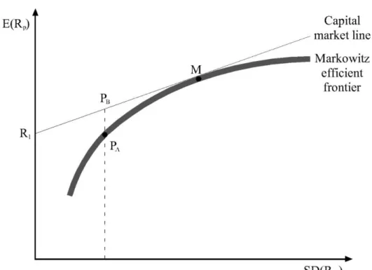
Professor Markowitz also add great contributions to distinguish efficient and inefficient porfolio selection concept. Efficient portfolios has a set of efficient mean-variance combinations, which reflects investors’ desired risk & return combinations. In other words, if a portfolio accepted as a efficient, it should offer more return with same or lower risk than other investment. Later, this phrase evolved into the efficient frontier. (Markowitz H. M., 1999). The efficient frontier is the plot that describes number of optimum portfolios which offer more expected return in given risk level. Two key important property the efficient frontier graph have. First, the graph is upward-sloping graph rather than straight line. Since the effect of allocation of the portfolio, their avarage standard deviation will be less than the single asset. Another important aspect is each point on the line stands for an optimal combination of the securities given level of risk. In other words, the point on the line symbolize the best portfolios. The below of the curve represent less efficient portfolios due to the fact that these portfolios don’t be diversified enought than the upper point on the curve.

(26)

13

X,Y, Z represent the points that includes more risk for the same level of the return on the curve. (Investing Answers, 2018)

Figure 3.3: Efficient Frontier

(Investing Answers, 2018)

Markowitz theory underlines the point that creating efficient portfolio doesn’t mean that it should include so many securities for diversification, it advocated that the portfolio need to include enough, well-selected securities. (Ş. Y. Yiğiter, 2017). Besided, Markowitz portfolio theory suggests that correlation between securities is not flawless. It means that securities’ price are able to act together under similar circumstances. So, before portfolio selection, positively related return of securitites do not added same portfolio for the account of eliminating risk. Basically, Markowitz portfolio theory assumes two steps before portfolio selection. First, combining information for the securities future performance with the scope of experiences. Second, is selection efficent portfolio.

(27)

14 3.3. CAPITAL MARKET THEORY

In the mid of 1960, Capital Market Theory was improved by William Sharpe within the scope of further work of Modern Portfolio Theory. This model start with exploring effect of risk-free asset. Although Sharpe was accepted the father of the theory, John Linter and John Mossin had great controbution to the theory with their individual works. Today, the theory is widely known as Sharpe-Linter-Mossin (SLM) Capital Asset Pricing Model. There are some key assumption on the Capital Market Theory:

 All investors are efficient. They make investment decision after considering expected return and risk.

 Investors accepted that they borrow or lend at the risk-free rate.

 Investors are rational and risk-averse and subcribe to Markowitz method of portfolio diversification. (J Fabozzi, 2001)

 Investors made their investment for the equal of time horizon.

 There are no transaction costs or no taxes or no inflation or no mispricing within the capital markets

 All investors expectations are homogenous.They have same probabilty of outcome. (Capital Market Theory, 2018)

Markowitz efficent portfolio was generated based on expected return and variance, and efficient portfolio was described as the portfolio which has lower variance while it provide same return level. In this regard, we are able to conclude that Markowitz Efficient Portfolio consist of risky asset. On the other hand, Capital Market Theory attirubute risk-free rate property into the former theory. Risk-free rate is theoretical rate which offer return on investment with zero-risk. It genereally provide lower rate of return due to fact that the rate don’t take additional risk. (Risk-Free Rate Of Return, 2018) It means that investors obtain higher return on his holdings only by incurring additional risk. (Sharpe, September 1964)

(28)

15

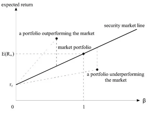
When we combine Markowizt efficient frontier with risk free rate, capital market line and Markowitz Efficient Frontier will be tangent at point M. All the point on the capital market line combines risk-free asset with risky assets. The slope of the line shows trade off between risk and return. Right of the M point represent more levereged portfolio than the right of the point since it includes more risky asset. When we compare same level of risk or standard deviation both Capital Market Line and Efficient Frontier at the point P_b and P_a , P_b point supply more higher return than the Pa on the same level of risk. It means that risk- averse investors would prefer P_b portfolio in their investments.

Figure 3.4: Capital Market Line

(29)

16 3.4. CAPITAL ASSET PRICING MODEL

Capital Asset Pricing is widely used model in finance which helps required rate of return on asset to make investment decision. Jack Treynor (1961-1962), William F. Sharpe (1964), John Linter (1965), evolved this theory with their individual work on the previous portfolio and Capital Market Theory. The main attribution of the Capital Asset Pricing model is adding systematic risk (non-diversifiable risk) into the model thanks to the term beta (β). It also includes expected return of the market and expected return of theoritical risk-free rate of return. As the previous theories, it accepts that overall risk consist of systematic (non-diversifiable) and unsystematic risk (diversifiable risk). The theory explains that required return of the asset and its systematic risk has linear relationship. There are some crucial assumption in the Capital Asset Pricing Model:

 All market is perfectly competitive: There are many investors and price movement cannot be changed or effected by individual investors.

 All investors are risk-averse and they have homogenous expectation.  Investors can borrow and lend at risk-free rate.

 Investors hold well-diversified portfolios: Investors eliminated unsystematic risk or ignored

 All market are frictionless: There are no transaction cost or tax for investment.

 There are perfect market condition: Information is reachable for all investors.

 All investors use single period of time: All the assets tested at same period of time to eliminate time effect on the model.

(30)

17 The empirical CAPM formula is:

(r_it− 𝑟_𝑓𝑡) = 𝛼_𝑖+ 𝛽_𝑖 (𝑟_𝑚𝑡 − 𝑟_𝑓𝑡) + ∈_𝑖𝑡

r_it: return of the stock i at time t, 𝑟_𝑓𝑡: risk-free rate at time t, 𝛼_𝑖: intercept term of stock i, 𝑟_𝑚𝑡: market return at time t, 𝛽_𝑖: beta of the stock i,

∈_𝑖𝑡: error term of the stock i at time t.

3.4.1. Market Risk Premium

Market risk premium is the excess return on the risk-free rate. It basically describes relationship with asset in the portfolio and theoritically excepted risk-free rate. Generally, investors use treasury bond-yield as a risk-risk-free rate. In Turkey, 2-year Treasury Bond yield accepted as a benchmark rate..

Market Risk Premium = (𝑟_𝑚𝑡 − 𝑟_𝑓𝑡)

3.4.2 Beta

Beta used as a risk metric in the CAPM model. It represent systematic risk or volatility comparing to the entire market. This beta value shows only individual assets or portolios’ risk and it is completely different from variance ( σ2_{), which} explains diversifiable part of risk.

(31)

18 𝛽_𝑖= 𝜎𝑖,𝑚

𝜎_𝑚2

While we intertpreting beta, square value must be taken into consideration. R-square show that percentage of explanatory level achived by regression. For this reason, it will not be logical to interpret beta as a risk indicator, if the regression R-square level is relatively low. (Investopedia, 2018) Theoritically, the market beta value is accepted as 1. As mentioned before, the performance of the portfolios compared according to the market risk exposure. Then, we are able to conclude that beta interperation can be made at these ways:

If Beta = 1: It means that the portfolio or stock exposure same amount of risk with the market. In other words, if the stock market rise up by 1%, the selected portfolio would be rise up by 1%

If 0 < Beta <1: It means that portfolio would not be affected by the fluctuation as the overall market. This portfolio or stocks are less volatile than the market.

If Beta > 1 : It means that the asset is more volatile than the overall market. It will fluctuated more than the market, so this accepted as more risky assets.

If Beta < 1 : It means that asset act perfectly different from the overall market. It means that if the overall market rise up 1%, the asset will be go down by 1%.

3.4.3. Security Market Line

The security market line accepted a characteritic Line, is a visiual explanation of the Capital Asset Pricing Model. The line illustrates expected return of a portfolio at given level of risk, while it takes into consideration risk-free rate.

(32)

19

Security market line based on systematic risk. Though it seems similar to Capital Market line, their risk measure is different from each other. Security Market Line uses Beta as the risk measure, whereas Capital Market Line uses stanadard deviation. We know that standard deviation stands for unsystematic risk or diversifiable risk. On the other hand, each point on the security market line represent expected return level versus market risk level or systematic risk level. Besided, security market line includes both efficient and non-eficient portfolios, while capital market line only illustrate efficient portfolios. Below of the security market line shows underperforming portfolios compared to the market, whereas above of the line shows outperforming portolios compared to the market.

(33)

20

3.5. TREYNOR AND MAZUY MARKET TIMING MODEL

Treynor and Mazuy introduce a unconditional model to estimate market timing ability of the investors in their article named “ Can mutual funds outguess the market” in 1966.

They assume that all investors would like to outguess the market. Each investor would like to create their portfolio with less volatile assets if they expect the market is going fall. On the other hand, if they expect the market is going to shift they do vice versa. First, they asked question before they conduct an experiment: “Is there a evidence that the volatiliy of the fund was higher in

years when the market did well than in years when the market did badly“

(Treynor & Mazuy, 1966) Within this scope, they improved CAPM by using quadratic term to explain market timing ability of the investors. The model mainly test whether the portfolio managers are able to adjust their position on time according to the expectation of fluctuation in the market.

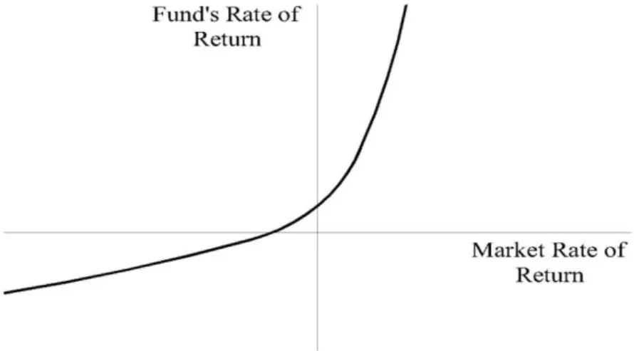
Figure 3.6. Characteristic Line for the fund which able to outguess the market better than average.

(34)

21

Traditional Capm theory indicates that expected return of the fund and market returns have linear relationship. However, Treynor and Mazuy indicated that they have a convex relatonship rather than linear. They illustrates this relationship by the line called The Charachteristic Line. The investors perfectly adjust their position whether market is bullish o bearish. Because of the perfect predict ability of the investors, the charachteristic line will have smoother, quadratic behaviour as the Figure 3.6. The convex behaviour of the line implies that the investor are able to perform market-timing ability, in this way they gain more return than normal, and change the systematic risk of the portfolio. (Treynor & Mazuy, 1966).

Treynor and Mazuy Market Timing Regression:

(r_it− 𝑟_𝑓𝑡) = 𝛼_𝑖+ 𝛽_𝑖(𝑟_𝑚𝑡− 𝑟_𝑓𝑡) + ɣ_𝑖(𝑟_𝑚𝑡− 𝑟_𝑓𝑡)2+∈ 𝑖

r_it: return on stock i at time t, 𝑟_𝑓𝑡: risk-free rate of return at time t, 𝛼_𝑖: selectivity ability,

ɣ_𝑖: the parameter measuring the market timing performance.

According to the theory, if the gamma (ɣ_𝑖) > 0, which is coefficient of the

(𝑟_𝑚𝑡− 𝑟_𝑓𝑡)2, the fund manager have market- timing ability. On the other hand, if the gamma (ɣ_𝑖) < 0, it means that fund managers don’t have market timing ability.

(35)

22 3.6. THE MODEL

The aim of this dissertation is that evaluting performance of the sectoral indices with Capital Asset Pricing Model and Treynor & Mazuy Market Timing Model in Turkey. It also means that evaluating performance of these theories under both crisis, pre-crisis and post-crisis conditions.

To the make this experiment, I used classical version of the Capital Asset Pricing Model as below formula:

(r_it− 𝑟_𝑓𝑡) = 𝛼_𝑖 + 𝛽_𝑖 (𝑟_𝑚𝑡 − 𝑟_𝑓𝑡) + ∈_𝑖𝑡

I used daily closing price of all indices, and calculate logaritmic return of both sectoral indices and market index as below formula:

𝑟𝑖𝑡 = 𝐼𝑛 ( 𝑝_𝑇 𝑝𝑇−1

)

𝑟_𝑚𝑡: logaritmic return of market index 𝑟_𝑖𝑡: logaritmic return of index p PT : closing price of index at time t

PT-1: closing price of the index at time (t-1)

I compare all the sectoral indices β and compare which indices swing more than the market, while for those of them which swing less than the market. As theoritically excepted, I assume that market beta is equal to 1.

For many work, alpha value is called excess return or abnormal return. I interpret α value as below comparision for the gauge for the market index explanatory capability at the given level of the regression, and called it as a abnormal return of the regression.

(36)

23

Alpha < 0 : If the α value is below zero, I interpret that the sectoral indicies provide less return comparing to its risk,

Alpha = 0 : If the α value equal to zero, I interpret that the sectoral indicies neither create nor destroyed value a the given risk level,

Alpha > 0 : If the α value above zero, I interpret that that the sectoral indicies provide more return compared to its risk.

To evaluate market timing of the investors, I used quadratic Treynor and Mazuy Market Timing Model as below:

(r_it− 𝑟_𝑓𝑡) = 𝛼_𝑖 + 𝛽_𝑖(𝑟_𝑚𝑡− 𝑟_𝑓𝑡) + ɣ_𝑖(𝑟_𝑚𝑡− 𝑟_𝑓𝑡)2+∈ 𝑖

I consider alpha and beta value as a market timing adjusted value of the CAPM, and analyze how it changed when the quadratic term added into the regression, and compared classical version of CAPM value of them.

As the theory accepted, I interpret that positive value of the gamma, which is the coefficient of the quadratic term of the excess return of the market, as the investors have market timing ability, whereas the negative value of the gamma as the non-timimig ability of the investors.

(37)

24

PART 4: DATA

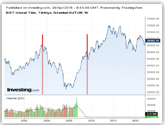
In the thesis, 23 of primary sectoral indices in BIST are analyzed. The closing price of the indices are obtained from Bloomberg Terminal, and all the calculations made in Microsoft Excel and Eviews. The experiment period is between January 3, 2004 and December 31, 2017. To make comparison, this data is divided into three parts: pre-crisis period as January 3, 2004 to October, 1 2007, crisis period as October 1, 2007 to December 31, 2010 and the post-crisis period January, 3 2011 to December 31, 2017. These division made with the help of Investing graph tool. The breaking points in the experiment represent the parts : the pre-crisis, the crisis and the post-crisis period.

Figure 4.1 XUTUM index movement between 2007 and 2012

(38)

25

Bist All Index, whose ticker symbol is XUTUM, is used as a market index. The index includes all traded stocks in Borsa Istanbul (BIST) except investment trusts. In the experiment, only BIST Spor Index (XSPOR) is started from April 1, 2004 due to fact fact that the index was introduced at that time.

Table 4.1. Sectoral Index Lists used in the experiment with ticker symbols

INDEX LIST SYMBOL

1 BIST BANKS XBANK.IS

2 BIST BASIC METAL XMANA

3 BIST INF. TECHNOLOGY XBLSM

4 BIST ELECTRICITY XELKT

5 BIST FINANCIALS XUMAL

6 BIST REAL EST. INV. TRUSTS XGMYO

7 BIST SERVICES XUHIZ

8 BIST HOLD. AND INVESTMENT XHOLD

9 BIST CHEM. PETROL PLASTIC XKMYA

10 BIST LEASING FACTORING XFINK

11 BIST NONMETAL MIN. PRODUCT XTAST

12 BIST BIST METAL PRODUCTS MACH. XMESY

13 BIST TRANSPORTATION XULAS

14 BIST INDUSTRIALS XUSIN

15 BIST INSURANCE XSGRT

16 BIST SPORTS XSPOR

17 BIST TECHNOLOGY XUTEK

18 BIST TEXTILE LEATHER XTEKS

19 BIST TELECOMMUNICATION XILTM

20 BIST W. AND RETAIL TRADE XTCRT

21 BIST TOURISM XTRZM

22 BIST WOOD PAPER PRINTING XKAGT

23 BIST FOOD BEVERAGE XGIDA

Since the experiment period’s duration is long, and market advancement in the early of 2000s is low, risk- free rate in Turkey are not able to be determined as of today’s norm. Though 2-year benchmark bond rate is accepted as a risk-free rate today because the 2-year bond was firstly issued in

(39)

26

2007, we cannot use this rate in the experiment. Instead of this, Interbank rate is accepted as a benchmark rate, and the data obtained from Central Bank of Turkey Database. The indices return calculated on daily basis, and all the returns on both CAPM and Treynor and Mazuy Market Timing Formula calculated as a logaritmic return.

(40)

27

PART 5: RESULTS

In the first section, Alpha (α), Beta (β) and R² values for each of sectoral indices come from both CAPM and Treynor& Mazuy Market Timing Model are determined, analiyzed under three-period scale: the pre-crisis, the crisis, the post-crisis. In the second section, each of indices market timing abilities explained with gamma(ɣ) values which come from Treynor&Mazuy Market Timing Model.

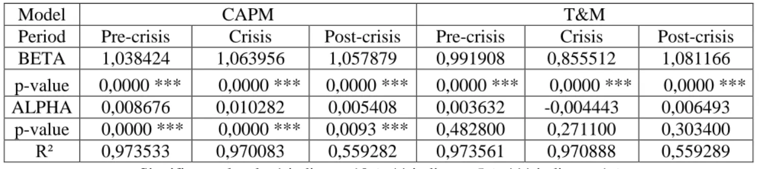
5.1. RESULTS FOR BIST BANK (XBANK) INDEX:

According to the Table 5.1, It can be seen that R-squared value relatively high during pre-crisis period and crisis period; the model successfully explained by independent variables at that periods, while it is considerably low on post-crisis periods. Hence, interpreting regression results on post-crisis period is not meaningful for both models. Beta values in CAPM for both period show that XBANK index more aggresive than the market index (XTUM) due to fact that its Beta is higher than 1. If the market index increase 1%, the index will be increase higher than 1, whereas if the market index decrease 1%, the XBANK index will be. It is also significant that Beta value at crisis period is higher than other periods, 1,063956. Conversely, Beta value come from Treynor and Mazuy model is considerably lower than 1, and it has lowest value at the crisis period. Additionally, Abnormal return values (alpha) are not significant at Treynor&Mazuy Model, while abnormal return in CAPM is significant at 1% level. The results indicates that XBANK index have positive abnormal return, and its highest abnormal return is in the crisis period, 0,010282. So, in the crisis period, XBANK made more return than expected based on its risk.

(41)

28

Table 5.1. CAPM and Treynor&Mazuy Regression results for XBANK

Model CAPM T&M

Period Pre-crisis Crisis Post-crisis Pre-crisis Crisis Post-crisis

BETA 1,038424 1,063956 1,057879 0,991908 0,855512 1,081166

p-value 0,0000 *** 0,0000 *** 0,0000 *** 0,0000 *** 0,0000 *** 0,0000 ***

ALPHA 0,008676 0,010282 0,005408 0,003632 -0,004443 0,006493

p-value 0,0000 *** 0,0000 *** 0,0093 *** 0,482800 0,271100 0,303400

R² 0,973533 0,970083 0,559282 0,973561 0,970888 0,559289

Significance levels: * indicates 10%, ** indicates 5%, *** indicates 1%

The Treynor and Mazuy Model analysis shows that XBANK index investors have positive market timing ability at the post-crisis periods, but the value is not significant at the periods Conversely, the investors have a negative market timing ability both at the crisis period and pre-crisis period, but only the crisis period is statistically significant at the 1% level.

Table 5.2. Market-timing regression coefficient results for XBANK

Pre-crisis Crisis Post-crisis

Gamma p-value R² Gamma p-value R² Gamma p-value R²

-0,1037 0,316 0,97356 -0,66 0,0001 *** 0,97089 0,11977 0,8554 0,55929 Significance levels: * indicates 10%, ** indicates 5%, *** indicates 1%

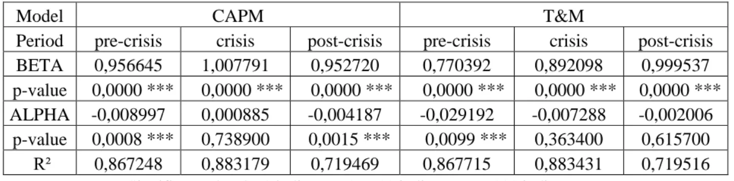
5.2. RESULTS FOR BIST BASIC METAL (XMANA) INDEX:

Each of models have relatively high R-squared value, it means that the variables in the models are explain the model successfully. The CAPM results shows that The Basic Metal Index have aggresive behaviour at the crisis period because the beta value is higher than 1. Also, it has positive abnormal return on the crisis period, but it is not statistically significant. All statistically significant abnormal values are negative. It proves that XMANA stocks created less return value than expected level of risk. According to the Treynor&Mazuy results, Beta, which

(42)

29

stands for systematic risk, reach its highest point at the post-crisis period, 0,999537. It is also significant that CAPM and Treynor and Mazuy result for Beta is relatively different from each other. Treynor&Mazuy model results point out that the index exposure apparently less risk than the market, while CAPM results show it is nearly as risky as the market.

Table 5.3. CAPM and Treynor&Mazuy Regression results for XMANA

Model CAPM T&M

Period pre-crisis crisis post-crisis pre-crisis crisis post-crisis

BETA 0,956645 1,007791 0,952720 0,770392 0,892098 0,999537

p-value 0,0000 *** 0,0000 *** 0,0000 *** 0,0000 *** 0,0000 *** 0,0000 ***

ALPHA -0,008997 0,000885 -0,004187 -0,029192 -0,007288 -0,002006

p-value 0,0008 *** 0,738900 0,0015 *** 0,0099 *** 0,363400 0,615700

R² 0,867248 0,883179 0,719469 0,867715 0,883431 0,719516

BIST Basic Metal index Treynor and Mazuy results show that the index have negative-timing ability on the pre-crisis period and it is significant at the 10% level. However, the index market timing ability coefficient (ɣ) is not significant at other periods.

Table 5.4. Market-timing regression coefficient results for XMANA

-0,4153 0,0661 * 0,86772 -0,3663 0,2801 0,88343 0,24079 0,5631 0,71952 Significance levels: * indicates 10%, ** indicates 5%, *** indicates 1%

(43)

30

5.3. RESULTS FOR BIST INFORMATION TECHNOLOGY (XBLSM) INDEX:

Except post-crisis period, all R-squared values are relatively high, in other words, the explaining capacity of the regression at these periods are enough. The beta coefficient value, which reflect systematic risk, is the highest point on the crisis period for Treynor and Mazuy Market Timing Model, 1,242076. It means that the index is %24 more volatile than the benchmark index. On the other hand, CAPM Beta coefficient is less than 1. It seems the index less volatile than the market, also its all abnormal return is negative and it is statistically significant.

Table 5.5. CAPM and Treynor&Mazuy Regression results for XBLSM

Model CAPM T&M

BETA 0,976334 0,961678 0,884737 0,768903 1,242076 0,556537

p-value 0,0000 *** 0,0000 *** 0,0000 *** 0,0000 *** 0,0000 *** 0,0000 ***

ALPHA -0,006311 -0,00582 -0,010967 -0,028803 0,013989 -0,026259

p-value 0,0024 *** 0,0160 ** 0,0000 *** 0,0010 *** 0,05330 * 0,0000 ***

R² 0,918469 0,893138 0,614314 0,919057 0,894781 0,616582

According to the Treynor&Mazuy Market Timing Model, BIST Information Technology Index have positive market-timing ability during crisis period with the 99% confidence level. On the other hand, it has negative timing ability both pre- and post-crisis periods with the 99% confidence level.

Table 5.6. Market-timing regression coefficient results for XBLSM

-0,4625 0,0084 *** 0,91906 0,88783 0,0038 *** 0,89478 -1,688 0,0006 *** 0,61658 Significance levels: * indicates 10%, ** indicates 5%, *** indicates 1%

(44)

31

5.4. RESULTS FOR BIST ELECTRICITY (XELKT) INDEX:

All regressions for both CAPM and Treynor&Mazuy has considerable high explanatory power, its R-squared value is range between 0,724546 and 0,824375.In the table 5.7, statistically significant alpha coefficients are negative. It means that the index has less return than expected at the regressions. All the Beta values are significant at the 1% level, and it illustrates that the index less fluctuate than the market index. Especially, the beta value in the Treynor and Mazuy Model seems considerably low in the post-crisis period, 0,640649.

Table 5.7. CAPM and Treynor&Mazuy Regression results for XELKT

Model CAPM T&M

Period Pre-crisis Crisis Post-crisis Pre-crisis Crisis Post-crisis BETA 0,947869 0,9679 0,944677 0,934825 0,907517 0,640649 p-value 0,0000 *** 0,0000 *** 0,0000 *** 0,0000 *** 0,0000 *** 0,0000 *** ALPHA -0,012003 -0,004643 -0,005824 -0,013417 -0,008909 -0,01999

p-value 0,0001 *** 0,1611 0,0000 *** 0,3136 0,3733 0,0000 *** R² 0,824375 0,817723 0,724546 0,824377 0,817792 0,72656

According to the Treynor and Mazuy Market Timing Model, none of market-timing coefficient is statistically significant except post-crisis period. At that period, XELKT index have negative market timing ability at the 1% significance level since its coefficient value is below zero, -1,56368. The portfolio which forming the index is not succesfully estimate the market fluctuation early.

Table 5.8. Market-timing regression coefficient results for XELKT

-0,0291 0,9124 0,82438 -0,1912 0,6513 0,81779 -1,56368 0,0001*** 0,72656 Significance levels: * indicates 10%, ** indicates 5%, *** indicates 1%

(45)

32

5.5. RESULTS FOR BIST FINANCIALS (XUMAL) INDEX:

All the regressions’ R-squared values are notably high at all the periods. It means that the all regressions almost perfectly explained by coefficients. Unlike Treynor and Mazuy values for Beta, CAPM value of the beta carry more risk compared to the benchmark index. The beta coefficient only above 1 at the post-crisis period for Treynor and Mazuy Model, whereas other periods it is below 1. In the crisis period, it is interesting that the index seems less risky than the market. When we look at the Alpha value, which stands for abnormal return, the regressions have positive abnormal return value except Treynor and Mazuy Model regression at the crisis period. It implies that the regressions have more excess return at the given level of risk.

Table 5.9. CAPM and Treynor&Mazuy Regression results for XUMAL

Model CAPM T&M

BETA 1,030468 1,049164 1,068064 0,997498 0,8635 1,042465

p-value 0,0000 *** 0,0000 *** 0,0000 *** 0,0000 *** 0,0000 *** 0,0000 ***

ALPHA 0,006725 0,007798 0,006486 0,00315 -0,005318 0,005293

p-value 0,0000 *** 0,0000 *** 0,0000 *** 0,0000 *** 0,0600 * 0,0114 **

R² 0,988229 0,984467 0,921716 0,988243 0,985134 0,921731

According to the Treynor and Mazuy Market Timing Abililty Model, the index have the negative market-timing ability at all period, but none of period- except the crisis period-statistically significant. In the crisis period, the index has negative market timing ability at the 1% significant level due to its gamma coefficient is below the 0.

(46)

33

Table 5.10. Market-timing regression coefficient results for XUMAL

-0,0735 0,2792 0,98824 -0,5879 0,0000 *** 0,985134 -0,13166 0,5457 0,921731 Significance levels: * indicates 10%, ** indicates 5%, *** indicates 1%

5.6. RESULTS FOR BIST REAL ESTATE INVESTMENT TRUST (XGMYO) INDEX:

According the regression results at Table 5.11, it is obvious that the regressions accounts for the model almost perfectly because of the fact that high R-squared value. Unlike the crisis period on The Treynor and Mazuy Model, the other periods beta below the benchmark index value, which is accepted that is equal to 1. It implies that the index generally less volatile or risky than the market. But in the crisis period, if the the market index expected to change 1%, the index will be either go up or go down more than by 1,18%. Besides that, all abnormal return values seems negative on the table, which mean that the return of the index will be less than the expectation at given risk level. The only positive alpha is in the Treynor and Mazuy crisis period, but it is not significant at any level.

(47)

34

Table 5.11. CAPM and Treynor&Mazuy Regression results for XGMYO

Model CAPM T&M

BETA 0,957883 0,962127 0,963928 0,89249 1,182164 0,613339

p-value 0,0000 *** 0,0000 *** 0,0000 *** 0,0000 *** 0,0000 *** 0,0000 *** ALPHA -0,009319 -0,006504 -0,00369 -0,01641 0,00904 -0,020026

p-value 0,0000 *** 0,0007 *** 0,0005 *** 0,0770 * 0,11630 0,0000 ***

R² 0,906971 0,929696 0,803752 0,907031 0,930749 0,806605

Treynor and Mazuy Regression Results illustrate that the index has negative market- timing ability in the post-crisis period with 99% confidence level. Conversely, the index market-timing ability is positive during the crisis period with 99% confidence level. Though the pre-crisis period it has negative timing-ability, it is not statistically significant.

Table 5.12 Market-timing regression coefficient results for XGMYO

-0,1458 0,4314 0,90703 0,69671 0,0043 *** 0,930749 -1,80315 0,0000 *** 0,806605 Significance levels: * indicates 10%, ** indicates 5%, *** indicates 1%

5.7. RESULTS FOR BIST SERVICES (XUHIZ) INDEX:

The results on the Table 5.13 shows that all the regressions have R-squared value, in other words, the variables successfully describes the regression. The beta values both come from CAPM and Treynor and Mazuy Market Timing Model is below the market index, between 0,855906 and 0,966147. But only the beta value on the Treynor and Mazuy Market Timing Model is relatively higher than the market index, 1,221269. It means that it is aggressive and riskier than

(48)

35

the market index (XUTUM) during crisis period. Besides, the index has provided a return that is lower according to its risk, since all the alpha values are negative except the crisis period on the Treynor and Mazuy Model but it is not meaningful at any given level.

Table 5.13. CAPM and Treynor&Mazuy Regression results for XUHIZ

Model CAPM T&M

BETA 0,966147 0,92931 0,891522 0,958621 1,221269 0,855906 p-value 0,0000 *** 0,0000 *** 0,0000 *** 0,0000 *** 0,0000 *** 0,0000 *** ALPHA -0,007326 -0,010954 -0,010543 -0,008142 0,00967 -0,012202

p-value 0,0000 *** 0,0000 *** 0,0000 *** 0,20300 0,0447 * 0,0000 *** R² 0,954299 0,94519 0,872905 0,95430 0,947213 0,872942

The result on the Table 5.14. illustrates that the BIST Services index has positive market-timing attitude during the crisis period with the 99% confidence level. On the other hand, both the pre-crisis and post-crisis the index have negative market-timing attitude, but they are not statistically meaningful at desired levels.

Table 5.14. Market-timing regression coefficient results for XUHIZ

-0,0168 0,8955 0,9543 0,92457 0,0000 *** 0,947213 -0,18318 0,4417 0,872942 Significance levels: * indicates 10%, ** indicates 5%, *** indicates 1%

(49)

36

5.8. RESULTS FOR BIST HOLDING AND INVESTMENT (XUHOLD) INDEX:

According to the regression results, all independent value in the regressions are able to stands for the depended variable almost perfectly, since the R-squared value is between 0,908033 and 0,971658. In the CAPM regressions, all the beta values- except post-crisis period- are above the market, 1,02031 and 1,013745, respectively. It illustates that the index more risky than the market at that periods. Controversely, the beta value is only above the market index beta, 1,091619, at the Treynor and Mazuy Market Timing Model post-crisis period. Moreover, the alpha value on the Treynor and Mazuy Model at the crisis period is considerably have negative effect on the return due to its value is -1%, and it is confident at the 99% level.

Table 5.15. CAPM and Treynor&Mazuy Regression results for XUHOLD

Model CAPM T&M

BETA 1,020301 1,013745 0,979632 0,98724 0,834249 1,091619

p-value 0,0000 *** 0,0000 *** 0,0000 *** 0,0000 *** 0,0000 *** 0,0000 ***

ALPHA 0,003998 0,00173 -0,001902 0,000413 -0,01095 0,003316

p-value 0,0013 *** 0,2200 0,0059 *** 0,9375 0,0097 *** 0,1128

R² 0,971644 0,964463 0,908033 0,971658 0,965117 0,908352

The results on the Table 5.16 indicates that the index have negative timing-ability during the crisis period, while it has positive timing-ability at the post-crisis period at the 1% significance level. However, the market timing coefficient is not statistically meaningful at the pre-crisis period.