A VARIATIONAL APPROACH TO THE PROBLEM OF OSCILLATIONS OF AN ELASTIC HALF CYLINDER
M. HASANSOY
Communicated by Mohammad Sal Moslehian Abstract. This paper is devoted to the spectral theory (more pre-cisely, to the variational theory of the spectrum) of guided waves in an elastic half cylinder. We use variational methods to inves-tigate several aspects of propagating waves, including localization (see Figure 1), existence criteria and the formulas to find them. We approach the problem using two complementary methods: The vari-ational methods for non-overdamped operator pencils to describe eigenvalues in definite spectral zones, and Ljusternik-Schnirelman critical point theory to investigate eigenvalues in the mixed spectral zone where the classical variational theory of operator pencils is not applicable.
1. Introduction and preliminary facts
Oscillations in an elastic continuum (see [10]) shaped like a semi-cylinder Q = R+
x1 × Ω ⊂ R3, Ω = {(0, x2, x3)}, are described by the
following system of partial differential equations: (1.1) 3 X k=1 ∂σik(v) ∂xk = ρ∂2vi ∂t2 , i = 1, 2, 3,
MSC(2010): Primary: 47A75; Secondary: 35p15, 34L15, 49R50
Keywords: Propagating waves, eigenvalue, variational principle, critical point. Received: 7 July 2010, Accepted: 4 October 2010
c
° 2012 Iranian Mathematical Society. 223
where v(t, x1, x2, x3) = (v1, v2, v3) and Ω ⊂ R2 is a bounded domain
with a smooth boundary, and
σ(v) = (σik(v))3i,k=1, σik(v) = λδikdivv + µ³ ∂vi
∂xk
+ ∂vk
∂xi
´
is the stress tensor. Here λ, µ > 0 are the Lame constants, ρ =
ρ(x2, x3) ∈ C( ¯Ω), and ρ > 0 is the density of the medium. We
con-sider a fixed boundary condition on the lateral surface Γ = R+x1 × ∂Ω:
(1.2) v|Γ= 0.
In this paper, all solutions of differential equations are obtained by sepa-ration of variables. That is, we look for weak solutions v(t, x1, x2, x3) of
the form eiwtW (x
1, x2, x3). By substituting this into equations (1.1) and
by using (1.2), we obtain steady-state oscillations of the semi-cylinder
Q: (1.3) 3 X k=1 ∂σik(W ) ∂xk + ρw 2W i = 0, i = 1, 2, 3,
with the condition on the lateral surface
W (x1, x2, x3)|Γ = 0.
Now we look for a solution to equation (1.3) of the form W (x1, x2, x3) =
e−ikx1u(x
2, x3). This assumption yields a two-parameter spectral
prob-lem in the space of vector-valued functions L3
2(Ω) := L2(Ω) ⊕ L2(Ω) ⊕ L2(Ω): L(k, w)u := (A + kB + k2C − w2R)u = 0, u|∂Ω= 0, (1.4) where A = − µ∆0 µ∆ + (λ + µ)D0 2 0 2 (λ + µ)D2D3 0 (λ + µ)D2D3 µ∆ + (λ + µ)D23 , B = −i(λ + µ) D02 D02 D03 D3 0 0 , C = λ + 2µ 0 00 µ 0 0 0 µ ,
R = ρ(x20, x3) ρ(x20, x3) 00 0 0 ρ(x2, x3) , ∆ = D22+ D32; Dk= ∂x∂k, k = 2, 3 and L2(Ω) = {f ¯ ¯ ¯RΩ|f |2dµ < ∞}. By
applying the boundary condition u|∂Ω= 0, we obtain the domain D(L)
of the unbounded operator pencil L. This domain, sometimes called the energetic space of the problem, is denoted by H := D(L). Clearly,
H = W01,2(Ω) ⊕ W01,2(Ω) ⊕ W01,2(Ω) (for facts on Sobolev spaces we cite [3]).
Now we define some spectral sets. Let k and w be complex numbers. We say that a complex number k is an eigenvalue (or wave number) and
w is a frequency (or eigen-frequency) if there is a 0 6= u ∈ L3
2(Ω) such
that
Au + kBu + k2Cu = w2Ru.
The spectrum of the operator pencil L(k, w) is defined as σ(L) :=
{(k, w)| 0 ∈ σ(L(k, w))}, where L(k, w) denotes the value of L at the
point (k, w). Define σw(L) := n k ¯ ¯ ¯(k, w) ∈ σ(L) o and σk(L) := n w ¯ ¯ ¯(k, w) ∈ σ(L) o
. In this paper, we investigate the varia-tional theory of eigenvalue spectra for the two parameter operator pen-cils L(k, w) defined in equation (1.4).
Many interesting and related problems have been investigated in the literature. Kostyuchenko and Orazov studied the structures of disper-sion curves k(w), how the motion of wave numbers k depends on w, and completeness problems for eigenvectors and associate vectors [10] (see also [8] for basis problems). A. A. Shkalikov recently studied similar questions for dissipative operator functions [11]. More general results in the abstract theory of regular waveguides may be found in [15]. How-ever, the questions of this paper are distinct from those examined in [10, 11] and [15]. Similar analyses of definite-type eigenvalues for ab-stract waveguides can be found in [1] and [2]. The main differences between the results of this paper and those given in [1,2] are as follows. i) We are interested in a concrete, real-valued mechanical problem and its associated two-parameter operator pencils.
ii) We set the problem in a real Hilbert space, which allows us to obtain deeper results in some cases.
iii) In the literature on nonlinear spectral problems, including [1] and [2], no spectral problems are studied in the mixed spectral zone
[δ−(w), δ+(w)] (see Figure 1 below). For the first time in the literature, we apply Ljusternik-Schnirelman critical point theory to obtain some results concerning this zone.
The main concern of this paper is propagating waves. In addition to finding solutions to the wave equation, we derive existence criteria and results concerning wave localization. The problem of finding frequencies
w for a fixed wave number k is an overdamped problem, so we use a
classical Poincar´e-Ritz type variational principle to describe the waves. However, the problem of finding wave numbers k for a fixed frequency
w in a definite spectral zone is not overdamped. In this case we use
other variational principles, such as that of Voss and Werner [13] and [7]. To study eigenvalues in a mixed spectral zone, we apply Ljusternik-Schnirelman critical point theory. There is currently no other method for studying eigenvalues in a mixed spectral zone, except for linear operator pencils of the form L(λ) = λA − B (see [4]).
Propagating waves are solutions of equation (1.1) in the form
v(t, x1, x2, x3) = u(x2, x3)ei(wt−kx1), where w and k are real numbers.
On the other hand v(t, x1, x2, x3) = u(x2, x3)ei(wt−kx1) is a solution of
(1.1) if and only if the triple (k, w, u) is a solution of the eigenvalue problem (1.4). Particularly, we are interested in neutral (resonance) pairs (k, u) for a fixed w. A pair (k, u), for a fixed w is said to be a neutral pair if 0 6= u ∈ H,
(1.5) Au + kBu + k2Cu = w2Ru and (L0(k)u, u) = 0, where L(k) := Au + kBu + k2Cu.
We start by deriving some facts about the operators A, B, C and
R defined above, which are very important to the investigation. The
original space for the problem is L3
2(Ω), and the energetic space where
we define the solution is H := W01,2(Ω)LW01,2LW01,2 or H = D(A12)
for Drichlet problems (see [10]). The following Proposition shows that the operators A, B, C and R are well defined on H. We extend the operator A by (Au, u) := (A12u, A
1
2u). In what follows, the notations
(u, v), kuk and ³
(u, v)H, kukH
´
denote the scalar product and norm in the space L3
2(Ω) (H), respectively.
Proposition 1.1. I) The operator A is a self-adjoint, positive-definite;
i.e., (Au, u) ≥ δ(u, u), for some δ > 0 and all u ∈ D(A) with the dis-crete spectrum,
II) The operators C and R are bounded and positive definite in L3 2(Ω).
III) The operator B is symmetric in L3
2(Ω) and |(Bu, v)| ≤ kukHkvk+ kvkHkuk, for all u, v ∈ H. In particular, this statement means that D(A12) ⊂ D(B).
IV)(the coercivity condition) (L(k)u, u) := (Au, u) + k(Bu, u) +
k2(Cu, u) ≥ kuk
H, for all u ∈ H.
Proof. I) The operator A is defined by
A = − µ∆0 µ∆ + (λ + µ)D0 2 0 2 (λ + µ)D2D3 0 (λ + µ)D2D3 µ∆ + (λ + µ)D32 .
Let u(x2, x3) = (u1(x2, x3), u2(x2, x3), u3(x2, x3) ∈ H ⊂ L32(Ω). Then Au = −¡µ∆u1, (µ∆ + (λ + µ)D22)u2+ (λ + µ)D2D3u3, (λ + µ)D2D3u2+ (µ∆ + (λ + µ)D2 3)u3 ´ . Hence, (Au, u) = −µ Z Ω ∆u1.¯u1dx − µ Z Ω ∆u2.¯u2dx2dx3− (λ + µ) Z Ω ∂2u2 ∂x2 2 ¯ u2dx2dx3− (λ + µ) Z Ω ∂2u3 ∂x2∂x3u¯2dx2dx3− (λ + µ) Z Ω ∂2u 2 ∂x2∂x3u¯3dx2dx3− µ Z Ω ∆u3.¯u3dx2dx3− (λ + µ) Z Ω ∂2u3 ∂x2 3 ¯ u3dx2dx3 = µ Z Ω |∇u1|2dx2dx3+ µ Z Ω |∇u2|2dx2dx3+ µ Z Ω |∇u3|2dx2dx3+ (λ + µ) hZ Ω ¯ ¯ ¯∂u2 ∂x2 ¯ ¯ ¯2dx2dx3+ Z Ω ¯ ¯ ¯∂u3 ∂x3 ¯ ¯ ¯2dx2dx3+ Z Ω ∂u3 ∂x3 ∂ ¯u2 ∂x2 dx2dx3+ Z Ω ∂u2 ∂x2 ∂ ¯u3 ∂x3 dx2dx3 i .
Now by using H¨older’s inequality we obtain Z Ω ∂u3 ∂x3 ∂ ¯u2 ∂x2dx2dx3+ Z Ω ∂u2 ∂x2 ∂ ¯u3 ∂x3 dx2dx3 = 2Re Z Ω ∂u3 ∂x3 ∂ ¯u2 ∂x2 dx2dx3≤ 2 hZ Ω ¯ ¯ ¯∂u3 ∂x3 ¯ ¯ ¯2dx2dx3 i1 2hZ Ω ¯ ¯ ¯∂u2 ∂x2 ¯ ¯ ¯2dx2dx3 i1 2 ≤ Z Ω ¯ ¯ ¯∂u2 ∂x2 ¯ ¯ ¯2dx2dx3+ Z Ω ¯ ¯ ¯∂u3 ∂x3 ¯ ¯ ¯2dx2dx3.
On the other hand Poincar´e inequality yieldsRΩ|∇u|2dx 2dx3≥ λ1(∆)
R
Ω|u|2dx2dx3. Consequently, (Au, u) ≥ 3µλ1(∆)kuk2, i.e., A is
L2(Ω) is compact (see [3]). This means that the spectrum of A is com-pact.
II) This property follows immediately from the definitions of opera-tors C and R.
III) The operator B is defined by
B = −i(λ + µ) D02 D02 D03 D3 0 0 . Now setting u = (u1, u2, u3), v = (v1, v2, v3) we can write
(Bu, v) = −i(λ + µ) hZ Ω (∂u2 ∂x2 + ∂u3 ∂x3)¯v1dx2dx3+ Z Ω ∂u1 ∂x2v¯2dx2dx3+ Z Ω ∂u1 ∂x3v¯3dx2dx3 i = i(λ + µ) hZ Ω ∂¯v1 ∂x2u2+ ∂¯v1 ∂x3u3dx2dx3 i − i(λ + µ) hZ Ω ∂u1 ∂x2¯v2dx2dx3+ Z Ω ∂u1 ∂x3¯v3dx2dx3 i .
From this formula by using H¨older’s inequality we obtain that |(Bu, v)| ≤
kukHkvk + kvkHkuk.
IV) This conclusion is standard in the spectral theory of the regu-lar waveguides (see [15], p. 44, for general hyperbolic equations in a
cylinder). ¤
Remark 1.2. It follows from Condition III) that the operator B is A-compact; i.e., A12BA12 is compact (see [9]). Condition IV) is often re-placed by the so-called energetic stability condition: (Au, u) + k(Bu, u) + k(Cu, u) ≥ (c0k2+ ζ)(Ru, u) for some c0 > 0, ζ > 0, which is stronger than the coercivity condition. In our case, this condition is also satisfied.
Proposition 1.1 means that the operator pencil L(k, w) is a pencil of the waveguide type (w.g.t.). A good resource on this subject is the book
Spectral Theory of Guided Waves by A. Silbergleit and Yu. Kopilevich
[15], which discusses a wide variety of waveguides. However, this book does not include any variational problems. The following theorem makes use of results given in Chapter 11 of [15].
Theorem 1.3. 1) The spectra σw(L) and σk(L) are discrete for a fixed complex w and complex k respectively,
2) The set σR(L) := {(k, w) ¯ ¯ ¯(k, w) ∈ σ(L), k ∈ R, w ∈ R} lies inside the hyperbola w2− c2 0k2 ≥ ζ,
3)There are no real eigenvalues if w <√ζ,
4) If w2 = ζ, then the only real eigenvalue permitted is k = 0. Zero will be an eigenvalue only if ζ is an eigenvalue of the problem Au = λRu,
5) (k, w) ∈ σ(L) and Imk = 0 imply Imw = 0.
For more information about localization problems for general operator functions, see [5].
2. Propagating waves: existence criteria, classification, and methods of finding them
As mentioned in the previous section,
v(t, x, x2, x3) = u(x2, x3)ei(wt−kx) is a propagating wave if and only if w, k are real and the equation
(2.1) Au + kBu + k2Cu = w2Ru,
has a nontrivial solution u ∈ H. Notice that u ∈ H is a solution of (2.1) if and only if
(A12u, A 1
2v) + k(Bu, v) + k2(Cu, v) = w2(Ru, v)
holds for all v ∈ H.
To classify all propagating waves for a fixed real w we need the fol-lowing definition.
Definition 2.1. We say that an eigenvalue k of the problem (2.1) (for a
fixed real w) is of positive (negative) type if (L0(k)u, u) > 0 ((L0(k)u, u) <
0) for all non-zero eigenvectors corresponding to k, respectively. Neutral pairs (k, w) are defined by (1.5). Let us fix w and define
p±(u, w) =
−(Bu, u)±pd(u, w)
2(Cu, u) ,
where d(u, w) = (Bu, u)2 − 4((A − w2R)u, u)(Cu, u). The
function-als p±(u, w) are the roots of the equation (Lw(k)u, u) = 0, u 6= 0.
Clearly, if k ∈ R is an eigenvalue and u 6= 0 is its corresponding eigenvector, then either p+(u, w) = k or p−(u, w) = k. Moreover, at
each eigenvector we have d(u, w) ≥ 0. Now we define two conic sub-sets, which will play an important role in finding the real eigenval-ues by variational principles: G(w) = {u ∈ H | d(u, w) > 0} and
d(u, w) ≥ 0} will also be the domain of the functionals p±(u, w). Let
Wp±(w) = {p±(u, w)|u ∈ G(w)} be the numerical range of p±(u, w) on
G(w). Now define the bounds of the ranges of p±(x, w) on G(w) and G0(w) as k−(w) = inf Wp−(w), k−0 (w) = infu∈G0(w)p−(u, w), k+(w) =
sup Wp+(w), k0+(w) = supu∈G0(w)p+(u, w), δ−(w) = inf Wp+(w),
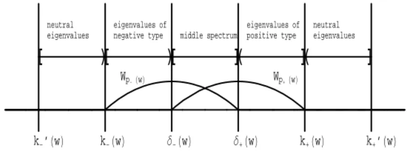
δ+(w) = sup Wp−(w). Notice that the inequalities k−0 (w) ≤ k−(w) ≤ δ−(w) ≤ δ+(w) ≤ k+(w) ≤ k0
+(w) hold for all two-parameter
op-erator pencils of waveguide type Only one inequality is not obvious:
δ−(w) ≤ δ+(w). Its proof for one-parameter, bounded operator pencils of waveguide type may be found in [2] (p. 1279). These inequalities will lead us to the distribution and a classification of real eigenvalues as in Figure 1. k-’HwL k-HwL ∆-HwL ∆+HwL k+HwL k+’HwL neutral eigenvalues neutral eigenvalues eigenvalues of negative type eigenvalues of positive type middle spectrum Wp- HwL Wp+ HwL
@
L@
L@
DH
DH
D
Fig 1. The distribution of the real eigenvalues.
Evidently, all mixed-type eigenvalues belong to the middle spectrum. The end intervals [k0
−(w), k−(w)) and (k+(w), k0+(w)] contain only
res-onance waves. All waves in [k−(w), δ−(w)) are outgoing, and all waves
in (δ+(w), k+(w)] are incoming. The middle interval [δ−(w), δ+(w)] may contain any kind of wave. The following theorem is about the structure of frequencies for a fixed real k.
Theorem 2.2. Let us fix k ∈ R. Then the following facts hold: 1) There are a countable number of real frequencies denoted by w±
n(k), which lie in the intervals [pζ + c2
0k2, +∞) and (−∞, −
p
ζ + c2 0k2]. 2) All real frequencies are described by
(2.2) w2n(k) = min L⊂H dim L=n max u∈L u6=0 (L(k)u, u) (Ru, u) , n = 1, 2, ..., where L(k) := A + kB + k2C.
3) w±n(k) → ±∞ for k → ±∞, and w+n(k)
λn → 1 for n → ∞. The
numbers λn, n = 1, 2, ..., are eigenvalues of the generalized eigenvalue problem Au = λRu.
Proof. 1) It follows from the statement 2) of Theorem 1.1.
2) In this case, eigenvalue problem (2.1) reduces to the generalized eigenvalue problem L(k)u = w2Ru. Therefore (2.2) is the Poincar´e-Ritz
principle for this problem, taking into account the fact that the domain of the operator pencil L(k) is the Sobolev space H.
3) We have L(k, w) ≥ (c2
0k2+ζ)R (see Remark 1.1). Then (L(k,w)u,u)(Ru,u) ≥
(c2
0k2+ ζ), and it follows from this inequality that wn±(k) → ±∞ for k → ±∞. Finally, by Proposition 1.1 we obtain that the spectra of the
operator pencils L(k, w) and A−12L(k, w)A−12 coincide. On the other
hand, the pencil A−12L(k, w)A−12 is a compact perturbation of the
op-erator A, and that is why wn+(k)
λn → 1 for n → ∞. (See [6, Chapter V],
[15, Theorem 13.1] and [9]). ¤
We remark that Figure 1 characterizes the distribution of real eigen-values for all regular waveguides, not just the half-cylinder (see [15] for similar results for abstract waveguides). However, for a specific problem one can obtain more results. For example, in our case all operators A, C and R transform real-valued functions to real-valued functions. But op-erator B maps real-valued functions to complex-valued functions. Using this fact we can simplify the problem as follows.
Let us consider a propagating wave v(t, x, x2, x3) = u(x2, x3)ei(wt−kx1).
There are two possible cases:
A) The function u(x2, x3) is a real-valued function in H;
B) The function u(x2, x3) a complex-valued.
For case A), it follows from the eigenvalue problem (2.1) that (2.3)
½
Au + k2Cu = w2Ru Bu = 0,
where u ∈ H and k, w ∈ R. One can therefore pose the following problem in the real-valued space H: find solutions to equation (1.1) of the form v(t, x, x2, x3) = u(x2, x3) cos(wt − kx1) and v(t, x, x2, x3) = u(x2, x3) sin(wt − kx1), where u ∈ H and k, w ∈ R. This problem is
equivalent to that posed in (2.3).
Our first observation for The case A), is given in the following theo-rem.
Theorem 2.3. a) (Bu, u) = 0 for an arbitrary real-valued function u ∈ H,
b) δ+(u, w) = δ−(u, w) = 0;
c) there are only a finite number of real eigenvalues for a fixed real w; all positive (negative) eigenvalues are of positive type (negative type), and arranged as
±k1±(w) ≥ ±k2±(w) ≥ ... ≥ ±k±n(w),
respectively. d) k0
−(w) = k−(w) and k+0 (w) = k+(w); i.e., [k0−(w), k−(w)) = ∅ and
(k+(w), k0+(w)] = ∅;
e) The only neutral (resonance) eigenvalue permitted is k = 0. Zero will be a neutral eigenvalue only if w2 is an eigenvalue of the generalized eigenvalue problem Au = w2Ru.
Proof. a) Using the integration by-parts in the space H = W01,2(Ω) ⊕
W01,2(Ω) ⊕ W01,2(Ω) yields (Bu, u) = −i(λ + µ) hZ Ω ¡ ∂u2 ∂x2 + ∂u3 ∂x3 ¢ u1dx2dx3+ Z Ω ∂u1 ∂x2u2dx2dx3+ Z Ω ∂u1 ∂x3 u3dx2dx3 i = −i(λ + µ) hZ Ω −∂u1 ∂x2 u2dx2dx3−∂u1 ∂x3 u3dx2dx3+ Z Ω ∂u1 ∂x2 u2dx2dx3+ Z Ω ∂u1 ∂x3 u3dx2dx3 i = 0. b) It follows from a) that
p±(u, w) = ±
s ¡
(w2R − A)u, u¢
(Cu, u) .
Hence, p+(u, w) ≥ 0 and p−(u, w) ≤ 0. By the definition of δ±(w), we obtain
δ+(w) = sup Wp− = sup{p−(u, w)|u ∈ G(w)} ≤ 0
and
δ−(w) = inf Wp+ = inf{p+(u, w)|u ∈ G(w)} ≥ 0.
On the other hand, δ−(w) ≤ δ+(w). Consequently, δ−(w) = δ+(w) = 0.
c) By Theorem 1.1, all eigenvalues of problem (2.3) belong to the in-terval h − √ w2−ζ c0 , √ w2+ζ c0 i
and σw(L) is discrete. These facts mean that
there is no finite concentration point of the spectrum σw(L). Conse-quently, there are only a finite number of eigenvalues in
h − √ w2−ζ c0 , √ w2+ζ c0 i .
The fact that all positive (negative) eigenvalues are of positive type (neg-ative type), respectively, follows from (L0(k)u, u) = (Bu, u)+2k(Cu, u) =
2k(Cu, u).
d) According to Figure 1 we have Lw(k) ≥ 0 for k ∈ [k0−(w), k−(w)) ∪
(k+(w), k+0 (w)]. Thus, the inequality
kLw(k)uk2≤ (Lw(k)u, u)kLw(k)k
holds. It follows from this inequality that all values of the functionals
p±(u, w) in the intervals [k0−(w), k−(w)) and (k+(w), k0+(w)] consist of
neutral eigenvalues. On the other hand, (L0
w(k)u, u) = 2k(Cu, u) 6= 0 for k 6= 0. Hence, there are no neutral eigenvalues on (−∞, 0) and (0, +∞).
This proves d).
e) This statement has already been proved in c). ¤
More generally, considering cases A) and B) together, we obtain the following result.
Theorem 2.4. a) All eigenvalues in [k−(w), δ−(w)), arranged in an
increasing order, are described by the following two principles ki−(w) = min L⊂G− dim L=i max u∈L p−(u, w), i = 1, 2, ..., n. ki−(w) = max L⊂H dim L=i−1 inf u∈G− u⊥L p−(u, w) i = 1, 2, ..., n,
where G−(w) = {u|u ∈ G(w), p−(u, w) < δ−(w)} . Similar formulas hold for the eigenvalues in (k+(w), k0+(w)].
b) For a fixed w ∈ R, the spectral set σw(L) is nonempty and k±(w) ∈ σw(L). Thus, at least two propagating waves always exist.
Proof. a) By Proposition 1.1, the pencil we are studying is a waveguide type operator pencil. Variational principles for real eigenvalues in the intervals [k−(w), δ−(w)) and (k+(w), k+0 (w)] have already been studied
for this case in [1,2], and [7]. Thus, a) holds.
b) Let us show that k−(w) is an eigenvalue. By definition k−(w) =
inf Wp−(w), there is a u−n ∈ G(w), un−= 1 such that p−(u−n, w) → k−(w).
Since ku−
nk = 1, there is a weakly convergent subsequence u−nm of u
− n.
Thus, u−
nm * u for m → ∞. Using the definition of p−(u, w), we get
0 ≤¡Lw(k−(w))u−nm, u − nm ¢ =¡(Lw(k−(w)) − Lw(p−(u−nm)))u − nm, u − nm ¢ ≤ kLw(k−(w)) − Lw(p−(u−nm, w))k. Hence, ¡ Lw(k−(w))u−nm, u − nm ¢ → 0 for
m → ∞ by continuity of Lw(k). On the other hand, since Lw(k−(w)) ≥ 0, we obtain kLw(k−(w))u−nmk 2 ≤¡L w(k−(w))u−nm, u − nm ¢ kLw(k−(w))k.
Taking the limit for m → ∞, we find that Lw(k−(w))u−nm → 0 and
consequently Lw(k−(w))u = 0. Thus, ∃u−nm, ku
−
nmk = 1, u
−
nm * u
and Lw(k−(w))u = 0. Evidently, u 6= 0; otherwise, k−(w) would be a point of continuous spectrum of the operator pencil Lw(k). But by
Theorem 1.1, the spectrum σw(L) is discrete. This contradiction means that u 6= 0 and Lw(k−(w))u = 0; i.e., k−(w) is an eigenvalue. By the
same argument, one can establish that k+(w) is an eigenvalue. ¤
3. Eigenvalues in the interval [δ−(w), δ+(w)]: A critical point
approach
In this section, we study eigenvalues in the interval [δ−(w), δ+(w)].
This part of the spectrum is known as the middle spectrum. We are not aware of any prior results from the literature in this spectral zone, which contains all mixed-type eigenvalues (but not only this type). First, we note that classical variational theory does not work in the zone [δ−(w), δ+(w)]. We suggest two methods. The first is to transform
this problem into an eigenvalue problem for a self-adjoint operator in a Krein space. Then, by using the methods given in [4], some eigenval-ues in [δ−(w), δ+(w)] may be found. The second way is to transform
problem (2.1) into an eigenvalue problem for a nonlinear operator in a real Hilbert space, and then apply Ljusternik- Schnirelman critical point theory (see [14]) to find neutral pairs in [δ−(w), δ+(w)]. In this paper, we take the second approach.
Recall that for a fixed w, a pair (k, u) is said to be a neutral pair if (3.1) Au + kBu + k2Cu = w2Ru and (L0(k)u, u) = 0, 0 6= u ∈ H, where L(k) := Au + kBu + k2Cu.
First, we are going to set the problem in a real-valued Hilbert space. Let (k, w) ∈ R × R and 0 6= u ∈ H satisfy (3.1). Setting u(x2, x3) = u1(x2, x3) + iu2(x2, x3) and B = iB0 into (3.1), where
B0= −(λ + µ) D02 D02 D03 D3 0 0 ,
we obtain
A(u1+ iu2) + ikB0(u1+ iu2) + k2(Cu1+ iCu2) = w2(Ru1+ iu2).
Consequently,
Au1− kB0u2+ k2Cu
1 = w2Ru1 Au2+ kB0u1+ k2Cu2 = w2Ru2.
This system may be written in the following operator-matrix form: µ A 0 0 A ¶ · u1 u2 ¸ + k µ 0 −B0 B0 0 ¶ · u1 u2 ¸ + k2 µ C 0 0 C ¶ · u1 u2 ¸ = w2 µ R 0 0 R ¶ · u1 u2 ¸ . Put ˜A = µ A 0 0 A ¶ , ˜B = µ 0 −B0 B0 0 ¶ , ˜C = µ C 0 0 C ¶ and ˜R = µ R 0 0 R ¶ and u = · u1 u2 ¸
. We then obtain a two-parameter spectral prob-lem in the form
(3.2) Au + k ˜˜ Bu + k2C = w˜ 2Ru,˜
where u ∈ H ⊕ H. In what follows, we assume that H consists of real-valued functions. We therefore have ˜A∗ = ˜A, ˜C∗ = ˜C, and ˜R∗ = ˜R.
Further, ˜B is a symmetric operator, since B∗
0 = −B0. All statements
(I-IV) given in Proposition 1.1 hold. Thus, we have a two-parameter, waveguide-type eigenvalue problem in the real Hilbert space X = H⊕H. Let (k, w) be a neutral eigen-pair for problem (3.2), corresponding to an eigenvector u. It follows from ( ˜L0(k)u, u) = 0 that k = −( ˜Bu,u)
2( ˜Cu,u).
Substituting this value into (3.2), we arrive at the nonlinear generalized eigenvalue problem in the form
(3.3) ( ˜Bu, u)2 4( ˜Cu, u)2Cu −˜
( ˜Bu, u)
2( ˜Cu, u)Bu + ˜˜ Au = w 2Ru.˜
Clearly, the F-derivative of the functional G(u) = 1
2[( ˜Au, u) − ( ˜Bu,u)2 4( ˜Cu,u)] is G0(u) = ( ˜Bu,u)2 4( ˜Cu,u)2Cu −˜ ( ˜Bu,u)
2( ˜Cu,u)Bu + ˜˜ Au. We also have F
0(u) = ˜Ru,
where F (u) = ( ˜Ru,u)2 . Thus, problem (3.3) is equivalent to the problem of finding the critical points of the functional F (u) restricted to the
level set N1 = {x¯¯G(u) = 1}. More precisely, we obtain the eigenvalue problem (3.4) F0(u) = 1 w2G0(u), u ∈ N1 or (3.5) F0(u) = λG0(u), u ∈ N1, where λ = 1 w2.
Our next step is based on the Ljusternik- Schnirelman critical point theory (see [14], Chapter 44 and Theorem 44.A). We are now going to give a simple description of this theory from the point of view of our problem. We start with the following definition.
Definition 3.1. Let X and Y be Banach spaces and A : X → Y be an operator (linear or nonlinear). We say that
i) The operator A is strongly continuous iff un * u implies Aun → Au, where un* u denotes weak convergence in X, and
ii) The operator A is bounded if A maps bounded sets into bounded sets.
Now consider F, G : X → R and F0, G0: X → X∗, where X∗ denotes
the adjoint of X. We give some basic properties of the functionals and their F-derivatives.
Proposition 3.2. The functionals F and G belong to C1(X, R); F and F0 are strongly continuous; G0 is bounded and uniformly continuous on bounded sets in X.
Proof. All of these properties can easily be checked using the properties of the operators A, B, C and R given in Proposition 1.1, Definition 3.1, and the fact that the embedding W01,2(Ω) ,→ L2(Ω) is compact. ¤
By Km denote the class of all compact, symmetric subsets K of N1 such that genK ≥ m. Here genK is defined as the smallest natural number n ≥ 1 for which there exists an odd and continuous function
f : K → Rn\ {0} (see [14] and [12]). Let
cm = sup L⊂Km
inf
u∈LF (u) m = 1, 2, ...
Now we use the Ljusternik-Schnirelman theory to show that cm > 0, m =
1, 2, ... and that all these numbers are eigenvalues of problem (3.5), i.e, that there exists um ∈ N1 such that
Moreover, we have F (um) = cm, which means that the numbers cm are critical levels for the functional F on N1.
Set critN1,cF := {u ∈ N1
¯ ¯
¯F0u = c G0u and F (u) = c}.
We start with the Palais-Smale condition, which is crucial to this the-ory. First define the tangential mapping T FN1(u) at the vector u ∈ N1 by hT F (u), hi := hF0(u), hi for all h ∈ T N
1(u), where T N1(u) denotes
the set of all vectors h tangent to N1 at the point u ∈ N1.
Definition 3.3. Let F, G ∈ C1(X, R) and N 1 = {u
¯ ¯
¯G(u) = 1}. We say
that the functional F satisfies the Palais-Smale condition with respect to N1 at a point c ∈ R if un ∈ N1, F (un) → c and kT F (un)k → 0 implies that un has a convergent subsequence in X.
It is known that (see [14], p.289, Theorem 43.C) under the conditions given in Proposition 3.1, we have T N1(u) = Ker(G0(u)). Now we are
ready to prove the following Proposition.
Proposition 3.4. The functional F (u) = ( ˜Ru,u)2 satisfies the Palais-Smale condition with respect to N1 at each 0 6= c ∈ R.
Proof. By definition T F (u) is a functional, which is defined only on
T N1(u). We extend this functional from T N1(u) to the whole space X
by
Du := F0(u) − F (u)G0(u). Evidently, hDu, hi = hF0(u), hi = hT F (u), hi, h ∈ T N
1(u); i.e., Du is
an extension of T F (u). Here, Du ∈ X∗ and hDu, hi (or hF0(u), hi, hT F (u), hi) denotes the value of functional Du (or F0(u), T F (u)) at
h ∈ X. In particular, this fact means that kT F (u)k ≤ kDuk. We
can also prove that kT F (u)k = |Duk. Indeed, hDu, ui = 0, u ∈ N1. Let P be the orthogonal projection from X to G0(u). Then a vector x ∈ X may be written in the form x = cu + P x. Therefore,¯¯hDu, xi¯¯ =
¯
¯hDu, P xi¯¯ = ¯¯hT F (u), P xi¯¯ ≤ kT F (u)k.kP xk ≤ kT F (u)k.kxk, i, e.,
kDuk ≤ kT F (u)k and consequently kDuk = kT F (u)k. Now let un ∈ N1, Dun → 0, and F (un) → c for c 6= 0. We need to prove that
un has a convergent subsequence in X. By Proposition 1.1, we have
(L(k)u, u) ≥ ckuk2
X for all u ∈ X and k ∈ R. On the other hand,
³
L¡−2(Cu,u)(Bu,u) ¢u, u
´
= hG0(u), ui = 2G(u). Thus, G(u) ≥ ckuk2
X for all u ∈ X. It immediately follows from this inequality that unis a bounded
sequence in X. Since X is a reflexive Banach space, we find that un has a weakly convergent subsequence: unk * u for some u ∈ ¯coN1, the
convex hull of N1. Now it follows from the strong continuity of F0 that F0(u
nk) → F0(u) as k → ∞. By Proposition 3.1, G0(un) is also bounded.
It follows from Dun= F0(un) − F (un)G0(un) that G0(un) = F 0(u n) − D(un) F (un) → F0(u) c .
Hence, we have unk * u and G0(unk) →
F0(u)
c . To prove that unk → u,
it is enough to show that kunkk → kuk. For the sake of simplicity, we
check it for the case u = 0. Thus, unk * 0 and G0(unk) →
F0(0)
c =
0. Again by Proposition 1.1, (L(k)u, u) ≥ ckuk2X for all u ∈ X and
k ∈ R. On the other hand,
³
L¡−2(Cu,u)(Bu,u) ¢u, u
´
= hG0(u), ui. This yields hG0(u), ui ≥ ckuk2X for all u ∈ X. Now, putting into this inequality
u = unk, we get hG0(unk), unki ≥ ckunkk2X. Finally, taking the limit as
k → ∞, we get kunkkX → 0. ¤
The next step in nonlinear eigenvalue problems is to prove the exis-tence of ”deformations”.
Definition 3.5. A set M ⊂ X allows Ljusternik-Schnirelman deforma-tions with respect to F and c ∈ R iff for each open set U in X such that critN1,cF ⊂ U , there exists a number ε(U ) > 0 and a contiuous mapping d : M × [0, 1] → M such that
i) d(u, 0) = u, u ∈ M , and
ii) F (u) ≥ c − ε, u ∈ M \ U implies F (d(u, 1)) ≥ c + ε.
It is known that the Palais-Smale condition for c 6= 0 guarantees this fact. Thus as a consequence of Proposition 3.2 (see [14], p. 331, Corollary 44.30), we have
Corollary 3.6. For each c 6= 0, the level set N1 allows Ljusternik-Schnirelman deformations d(u, t) : N1 × [0, 1] → N1 with respect to c and F . Further, d is odd; i.e., d(−u, t) = −d(u, t).
Another important corollary of Palais-Smale condition is the following fact.
Corollary 3.7. The set critN1,cF is compact for all c > 0.
Proof. By definition critN1,cF := {u ∈ N1
¯ ¯
¯F0(u) = c G0(u) and F (u) =
c}. Let un ∈ critN1,cF . Then we have F (un) = c and T F (un) = 0.
It follows from the Palais-Smale condition that un has a convergent
To end the paper, we present our main theorem.
Theorem 3.8. Let cm = supL⊂Kminfu∈LF (u), m = 1, 2, · · · . Then:
i) critN1,cmF 6= ∅; i.e., there exists um ∈ N1 and λm ∈ R such that
F0(um) = λmG0(um) m = 1, 2, ..., ii) λm= cm, m = 1, 2, · · · .
Proof. Let critN1,cmF = ∅. Clearly, cm > 0, m = 1, 2, ..., since
F (u) > 0, u ∈ N1. Then by Proposition 3.2, F satisfies the Palais-Smale
condition with respect to N1 and cm. By Corollary 3.1, N1 allows con-tinuous and odd deformations d : N1× [0, 1] → R. We can choose U = ∅
in Definition 3.3, because we assume critN1,cmF = ∅. Then by Corollary
3.1, there exists an odd and continuous function d : N1× [0, 1] → R such
that F (u) ≥ cm− ε, u ∈ N1 implies F (d(u, 1) ≥ cm+ ε. By definition cm = supL⊂Kminfu∈LF (u), m = 1, 2, .... Thus, there exists K ⊂ Km,
such that F (u) ≥ cm− ε, u ∈ K. By statement ii) of Definition 3.3 and
Corollary 3.1, we get F (d(K, 1)) ≥ cm+ ε and d(K, 1) ∈ Km because d is odd and continuous. Let d(K, 1) = K1. Then we have infK1F (u) ≥ cm + ε. This fact means that supL⊂Kminfu∈LF (u) ≥ cm + ε, which
contradicts cm = supL⊂Kminfu∈LF (u), m = 1, 2, · · · .
ii) We have F0(u
m) = λmG0(um) and um∈ N1. Then hF0(um), umi = λmhG0(um), umi. Consequently, F (um) = λmG(um). Since F (um) = cm
and G(um) = 1, we obtain cm = λm. ¤
Finally, recall that we have concentrated our attention on the problem
F0(u) = λG0(u), u ∈ N1.
But the problem of finding of neutral pairs (k, u) for an operator pencil ˜
Lw(k) at fixed w ∈ R is described by the equation
(3.6) ( ˜Bu, u)2 4( ˜Cu, u)2Cu −˜
( ˜Bu, u)
2( ˜Cu, u)Bu + ˜˜ Au = w 2Ru.˜
This is the same as
F0(u) = 1
w2G0(u), u ∈ N1.
Using the connection λ = w12 and (3.4), we can state the following.
Corollary 3.9. Problem (3.6) has infinitely many eigenvalues w2 mwhich correspond to eigenvectors um such that
a) w12
m = cm= supL⊂Kminfu∈LF (u),
b) F (um) = w12
c) w2 m→ ∞. d) ³ −( ˜Bum,um) 2( ˜Cum,um), um ´
will be a neutral eigen-pair for problem 3.2 at w = wm.
References
[1] Y. Abramov, Two parameter operator pencils of waveguide type, Dokl. Math. 286 (1986), no. 4, 777–781.
[2] Y. Abramov, Pencils of waveguide type and related extremal problems, J. Soviet
Math. 64 (1993), no. 6, 1278–1289.
[3] R. A. Adams and J. J. F. Fournier, Sobolev Spaces, Elsevier/Academic Press, Amesterdam, 2003.
[4] P. Binding, R. Hryniv and B. Najman, A variational principle in Krein space II.
Integral Equations Operator Theory 51 (2005), no. 4, 477–500.
[5] M. I. Gil, Operator Functions and Localization of Spectra, Lecture Notes in Math-ematics, 1830. Springer-Verlag, Berlin, 2003.
[6] I.Gohberg and M. Krein, Introduction to the Theory of Linear Non-Selfadjoint Operators in Hilbert Space, Izdat, Moscow, 1965.
[7] M. Hasanov, Spectral problems for operator pencils in non-separated root zones,
Turk. J. Math. 31 (2007) 43-52.
[8] M. Hasanov, Basis problems for matrix valued functions, J. Math. Anal. Appl. 342 (2008) 766-772.
[9] T. Kato, Perturbation Theory for Linear Operators, Springer-Verlag, Berlin, 1995.
[10] A. G. Kostyuchenko and M. B. Orazov, The problem of oscillations of an elastic half cylinder and related selfadjoint quadratic pencils, J. Soviet Math. 33 (1986) 1025–1065.
[11] A. A. Shkalikov, On perturbation theory for points of the discrete spectrum of dissipative operator functions, Differ. Equ. 45, (2009), no. 4, 580-590.
[12] M. Struwe, Variational Methods, Applications to Nonlinear Partial Differential Equations and Hamiltonian Systems, Fourth Edition, Springer-Verlag, 2008. [13] H. Voss and B. Werner, A minimax principle for nonlinear eigenvalue problems
with applications to nonoverdamped systems, Math. Methods Appl. Sci. 4 (1982), 415–424.
[14] E. Zeidler, Nonlinear Functional Analysis and its Applications, Vol III., Varia-tional Methods and Optimization, Springer-Verlag, 1985.
[15] A. Zilbergleit and Y. Kopilevich, Spectral Theory of Guided Waves, IOP Pub-lishing, Bristol, 1996.
Mahir Hasansoy
Department of Mathematics, Dogus University, Acibadem/Kadik¨oy, Istanbul, Turkey Email: [email protected]