C om mun. Fac. Sci. U niv. A nk. Ser. A 1 M ath. Stat. Volum e 67, N umb er 1, Pages 310–316 (2018) D O I: 10.1501/C om mua1_ 0000000852 ISSN 1303–5991
http://com munications.science.ankara.edu.tr/index.php?series= A 1
ANALYSIS OF TWO DIMENSIONAL PARABOLIC EQUATION WITH PERIODIC BOUNDARY CONDITIONS
VILDAN GÜLKAÇ AND ·IREM BA ¼GLAN
Abstract. In this paper two dimensional parabolic equation with Dirichlet type boundary condition is considered. The existence and uniqueness of so-lution are shown. Also we construct an iteration algorithm for the numerical solution of this problem.
1. Introduction Consider the following mixed problem:
@u @t = @2u @x2 + @2u @y2 + f (x; y; t) ; (1) (x; y; t) : = f0 < x < ; 0 < y < ; 0 < t < T g u(0; y; t) = u( ; y; t) = 0 ; t [0; T ] (2) u(x; 0; t) = u(x; ; t) = 0 ; t [0; T ] (3) u(x; y; 0) = '(x; y) ; x [0; ] (4)
for a two dimensional parabolic equation with the Dirichlet type boundary con-dition. The function '(x; y) and f (x; y; t) are given functions on [0; ] and respectively. Denote the solution of problem (1)-(4) by u(x; y; t):
Two dimensional parabolic equation arise in many areas of science and engineer-ing and wide scope and applications in heat conduction [5, 6, 7] .Srivastava et al [1] discuss analytical solutions of two-dimensional rectangular heat equation. The description of various numerical and other methods with useful bibliography may be found in the surveys of [8, 2, 3] .Compact di¤erence scheme for solving wave equations in two-space dimensions is discussed in [4] .
In this study we prove the existence,uniqueness of the solution and we constract an iteration algorithm for the numerical solution . We will use Fourier method for the considered problem (1)-(4) .
Received by the editors: May 05, 2016; Accepted: May 30, 2017. 2010 Mathematics Subject Classi…cation. 35K55, 35K70, 65N30.
Key words and phrases. Parabolic equation, Dirichlet problem, iteration algorithm.
c 2 0 1 8 A n ka ra U n ive rsity C o m m u n ic a tio n s d e la Fa c u lté d e s S c ie n c e s d e l’U n ive rs ité d ’A n ka ra . S é rie s A 1 . M a th e m a t ic s a n d S t a tis t ic s .
The paper is organized as follows. In Section 2, the existence and the uniqueness of the solution of the problem are proved by using the Fourier method and iteration method. In Section 3, stability of method for the solution is shown. In Section 4, stability of method for the solution is given. In Section 5, the numerical procedure for the solution of the problem is given.
2. Existence and uniqueness of the solution
The main result on the existence and uniqueness of the solution of problems(1)-(4) is presented as follows.
We have the following assumptions on the data of problems (1)-(4).
(F 1) Let the function f (x; y; t) be continuous with respect to all arguments in and f (x; y; t) L2([0; ] [0; ]) :
(F 2) '(x; y) C ([0; ] [0; ]) :
By applying the standard procedure of the Fourier method, we obtain the fol-lowing representation for the solution of (1)-(3).
u(x; y; t) = 1 X m;n=1 Cmnsin mx sin ny Cmn(t) = 'mne ( m2+n2)t + t Z 0 Z 0 Z 0 e (m2+n2)(t )f ( ; ; ) sin mx sin ny d d d u(x; y; t) = 1 X m;n=1 'mne (m 2+n2)t sin mx sin y + 1 X m;n=1 0 @ t Z 0 fmn( )d 1 A sin mx sin ny (5) where 'mn= 42 Z 0 Z 0
'(x; y) sin mx sin nydxdy;
fmn=
Z
0
Z
0
e (m2+n2)(t )f ( ; ; ) sin mx sin nyd d :
Under the assumptions (F 1) and (F 2) ,the solution u(x; y; t) of the problems (1)-(4) is a unique solution.
3. Continuous dependence upon the data
The following result on continuously dependence on the data of the solution of (1)–(4) holds.
Theorem 1. = f'; fg satisfy the assumptions (F 1)-(F 2) of theorem 1 then the solution of the problem (1)-(4) depends continuously upon the data f; ':
Proof. Let = f'; fg and = '; f be two sets of the data, which satisfy the assumptions (F 1)-(F 2): Let us denote k k = (k'kC2;2([0; ]X[0; ])+ kfkC2;2;0( )): u u = 1 X m;n=1 ('mn 'mn) e (m 2+n2)t sin mx sin ny + 1 X m;n=1 0 @ t Z 0 Z 0 Z 0 e (m2+n2)(t ) f ( ; ; ) f ( ; ; ) sin mx sin ny d d d 1 A sin mx sin ny ku uk p1 6 k' 'k + T f f where T > 0: ku uk p1 6 For ! then u ! u:
4. Fully Implicit Backward-Difference Scheme
Consider the following advection-dispersion equation with forcing function f (x; y; t) : Using …ve point di¤erence scheme and fully implicit backward-di¤erence equa-tion, we obtain the following discrete form for (1)-(4).
un+1i;j = t h2
n
u(n+1)i 1;j + u(n+1)i+1;j + u(n+1)i;j 1 + u(n+1)i;j+1 o + h 2 t 4 u (n) i;j + h2f (n) i;j
and than this equation can be write ru(n+1)i 1;j + 1 2+ 2r u (n+1) i;j ru (n+1) i+1;j ru (n+1) i;j 1 + 1 2+ 2r u (n+1) i;j ru (n+1) i;j+1 = u(n)i;j + h2fi;j(n) (6)
and equation (6) can be written matrix form as, let (i) = (j) = 0 B B B B B B @ r 12+ 2r r 0 ::: 0 r 12 + 2r r 0 .. . . .. 0 ::: r 1 2+ 2r r u(n+1)0;j u(n+1)1;j .. . u(n+1)N;j 1 C C C C C C A + 0 B B B B B B @ r 12+ 2r r 0 ::: 0 r 12+ 2r r 0 .. . . .. 0 ::: r 12+ 2r r u(n+1)0;j u(n+1)1;j .. . u(n+1)N;j 1 C C C C C C A = u(n)i;j + h2fi;j(n) Aun+1i + Aun+1j = u(n)i;j + h2fi;j(n)
A[un+1i + un+1j ] = u(n)i;j + h2fi;j(n) (7) and with boundary conditions
u(0; y; t) = u( ; y; t) = u(x; 0; t) = u(x; ; t) = equation (7) can be written as
[un+1i + un+1j ] = A 1u(n)i;j + A 1h2fi;j(n)
from superposition principle equation (7) is equivalent to the (8) equation
un+1i + un+1j = u(n+1)i;j (8) Computationally, the implicit method de…ned by (8) can now solved by the following iterative scheme. At time t = tn+1:
Step 1: Solve the problem in the x direction for each …xed yjto obtain an
intermediate solution un+
1 2
i;j :
Step 2: Then solve it in the y direction for each …xed xi:
The initial and boundary conditions for numerical solution un+1i;j and uni;j are de…ned from the given initial and boundary conditions.
5. Stability of Method
Theorem 2. (Gerschgorin’s Theorem) The largest eigenvalues of the square matrix A module does not exceed the total of any row or column modules for any of the terms.
Proof. Let i be an eigenvalue of the N N matrix A, and xi the corresponding
eigenvector with components 1; 2; :::; s:Then the equation
Axi= xi in detail, is a1;1v1+ a1;2v2+ + a1;nvn = iv1 a2;1v1+ a2;2v2+ + a2;nvn = iv .. . as;1v1+ as;2v2+ + as;nvn = ivs .. . an;1v1+ an;2v2+ + an;nvn = ivn
Let vsbe largest in modulus of v1; v2; :::; vn. Select the sth equation and divide by
vs, giving i= as;1( v1 vs ) + as;2( v2 vs ) + + as;n( vn vs ) therefore vi vs 1 i = 1; 2; :::; n:
Theorem 3. (Brauer’s Theorem) Let Ps be sum of the moduli of the terms along
the sth row excluding the diagonal element as;s Then every eigenvalue of A lies
inside or on the boundary of at least one of the circles. j as;sj = Ps:
Proof. The proof of the Gerschgorin’s theorem
i= as;1( v1 vs ) + as;2( v2 vs ) + + as;s+ as;n( vn vs ) hence j i as;sj = as;1( v1 vs ) + as;2( v2 vs ) + + 0 + as;n( vn vs ) j i as;sj jas;1j + jas;2j + ::: + 0 + ::: + jas;nj j i as;sj Ps
this completes the proof.
Application of Brauer’s theorem to this A matrix with as;s= r and Ps= 2r
shows that its eigenvalues lie on or within the circle j j Ps
using Fig.1. 1 = r( + 2) and 2= r( + 2) and for stability j 1j 1 and
j 2j 1:
For j 1j 1
1 r( + 2) 1 ) r 1
For j 2j 1
r 1
( + 2) For overall stability r 1
( +2):
The …nite di¤erence equations will be stable when the modulus of every eigen-value of A 1 does not exceed one, that is when
1
1 ) 1
1
proving that the equations are unconditionally stable as 1 for all values of r.
6. Numerical Examples
If we consider the advection-dispersion equation (1)-(4) with initial conditions u(x; y; 0) = Si nx: Si ny:(1 x)2:(1 y)2; x; y 2 [0; ] x [0; ]
and forcing function
f (x; y; t) = (1 + 2xy) e tx3y3:6 and Dirichlet boundary conditions on [0; ] x [0; ] in the form
u(0; y; t) = u( ; y; t) = 0 u(x; 0; t) = u(x; ; t) = 0 for all t 0:
The exact solution to this two-dimensional advection-dispersion equation is where u(x; y; t) = etSi nx: Si ny:(1 x)2:(1 y)2
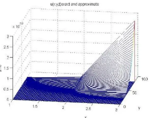
Figure 1 shows exact solutions and numerical solutions with t = 10001 ; h = 50 for t 2 [0; 1] :
From Figure 1 ,it can be seen that the numerical results are in good agreement with theoretical results. Speci…cally, for homogeneous Dirichlet boundary condi-tions , we have
un+10;j = u(0; yj; tn+1) = 0; un+1m;j = u( ; yj; tn+1) = 0
Figure 1. Exact solutions and numerical solutions with t =
1
1000; h = 50 for t 2 [0; 1] :
References
[1] Srivastava, H.M., K.Y. Kung and K.-J.Wang, Analytical solution of a two-dimensional recten-gular heat equation, Russian Journal of Mat. Physics,14,115-119, 2007.
[2] Furzeland, R.M., A comparative study of numerical methods for moving boundary problems, J.Ins.Math.Appl., 26, 411, 1980.
[3] Crank, J., Numerical methods in heat transfer, John Wiley, 9, 1981.
[4] Ran, M. and Zhang, C., Computers Math.with Appl.,Compact di¤erence scheme for a class of fractional in-space nonlinear damped wave equations in two space dimen-sions,71,1151,1162,2016.
[5] Cannon J.R., The solution of the heat conduction sub ject to the speci…cation of energy, Quart. Appl. Math., Vol.21, 155-160, 1983.
[6] Choi Y.S. and Chan K.Y., A parabolic equation with a nonlocal boundary condition arising from electrochemistry, Nonlinear Analysis, Vol.18,317-331,1992.
[7] Sharma P.R. and Methi G., Solution of two dimensional parabolic equation sub ject to Non-local conditions using homotopy Perturbation method, Jour. of App.Com. Sci., Vol.1, 12-16, 2012.
[8] Sak¬nc I., Numerical Solution of a Quasilinear Parabolic Problem with Periodic Boundary Condition, Hacettepe, Journal of Mathematics and Statistics, 39(2), 183-189, 2010.
Current address : Vildan Gülkaç: Kocaeli Uni.,Science and Arts Fac.,Department of Math.41380 Kocaeli TURKEY
E-mail address : [email protected]
ORCID: http://orcid.org/0000-0001-6284-1057
Current address : ·Irem Ba¼glan: Kocaeli Uni.,Science and Arts Fac.,Department of Math.41380 Kocaeli TURKEY
E-mail address : [email protected]