RECEIVER DESIGN AND PERFORMANCE
ANALYSIS FOR CODE-MULTIPLEXED
TRANSMITTED-REFERENCE ULTRA-WIDEBAND
SYSTEMS
a thesis
submitted to the department of electrical and
electronics engineering
and the institute of engineering and sciences
of bilkent university
in partial fulfillment of the requirements
for the degree of
master of science
By
Mehmet Emin Tutay
August 2010
I certify that I have read this thesis and that in my opinion it is fully adequate, in scope and in quality, as a thesis for the degree of Master of Science.
Asst. Prof. Dr. Sinan Gezici (Supervisor)
I certify that I have read this thesis and that in my opinion it is fully adequate, in scope and in quality, as a thesis for the degree of Master of Science.
Prof. Dr. Orhan Arıkan
I certify that I have read this thesis and that in my opinion it is fully adequate, in scope and in quality, as a thesis for the degree of Master of Science.
Asst. Prof. Dr. ˙Ibrahim K¨orpeo˘glu
Approved for the Institute of Engineering and Sciences:
Prof. Dr. Levent Onural
ABSTRACT
RECEIVER DESIGN AND PERFORMANCE
ANALYSIS FOR CODE-MULTIPLEXED
TRANSMITTED-REFERENCE ULTRA-WIDEBAND
SYSTEMS
Mehmet Emin Tutay
M.S. in Electrical and Electronics Engineering
Supervisor: Asst. Prof. Dr. Sinan Gezici
August 2010
In transmitted-reference (TR) and frequency-shifted reference (FSR) ultra-wideband (UWB) systems, data and reference signals are shifted relative to each other in time and frequency domains, respectively. The main advantage of these systems is that they remove strict requirements of channel estimation. In order to implement TR UWB systems, an analog delay line, which is difficult to build in an integrated fashion, is needed. Although FSR systems require frequency conversion at the receiver, which is much simpler in practice, they have data rate limitations. Instead, a code-multiplexed transmitted-reference (CM-TR) UWB system that transmits data and reference signals using two distinct orthogonal codes can be considered. This system requires a simpler receiver and has better performance than TR and FSR.
In the first part of the thesis, CM-TR systems are investigated and proba-bility of error expressions are obtained. For the single user case, a closed-form expression for the exact probability of error is derived. For the multiuser case, a closed-form expression is derived based on the Gaussian approximation, and the
results are compared in different scenarios. In the second part of the thesis, some optimal and suboptimal receivers are studied. First, low complexity receivers, such as the blinking receiver (BR) and the chip discriminator, are presented. The requirements for these types of receivers are explained, and the conditions under which their performance can be improved are discussed. Then, an analytical analysis of the linear minimum mean-squared error (MMSE) receiver and the re-quirements to implement this MMSE receiver are provided. Lastly, the optimal maximum-likelihood (ML) detector is derived, which has higher computational complexity and more strict requirements than the other receivers. Finally, sim-ulation results are presented in order to verify the theoretical results and to compare the performance of the receivers.
Keywords: Ultra-wideband (UWB), impulse radio (IR), multiple-access inter-ference (MAI), transmitted-reinter-ference (TR), frequency-shifted reinter-ference (FSR), coded-multiplexed transmitted-reference (CM-TR), blinking receivers (BR), chip discriminator, linear MMSE, maximum-likelihood (ML).
¨
OZET
KOD C
¸ O ˘
GULLAMALI VE REFERANS ˙ILET˙IML˙I C
¸ OK GEN˙IS
¸
BANTLI S˙ISTEMLER ˙IC
¸ ˙IN ALICI TASARIMI VE
PERFORMANS ANAL˙IZ˙I
Mehmet Emin Tutay
Elektrik ve Elektronik M¨
uhendisli˘
gi B¨
ol¨
um¨
u Y¨
uksek Lisans
Tez Y¨
oneticisi: Asst. Prof. Dr. Sinan Gezici
A˘
gustos 2010
Referans iletimli ve frekans kaydırmalı ¸cok geni¸s bantlı sistemlerde veri ve refer-ans i¸saretleri birbirlerine g¨ore zaman ve frekans b¨olgelerinde kaymı¸s bi¸cimdedir.
Bu sistemlerin en b¨uy¨uk avantajı, kanal tahmini ile ilgili zorlu isterlerin
kaldırılmasıdır. Referans iletimli ¸cok geni¸s bantlı sistemlerde, t¨umdevrelerde kullanılması zor olan analog gecikme hattına ihtiya¸c duyulmaktadır. Frekans kaydırmalı referans sistem alıcılarında ise pratikte ¸cok daha basit olan frekans ¸cevrimi i¸slemi gerekmesine ra˘gmen, bu sistemlerde veri hızı ile ilgili sınırlamalar
bulunmaktadır. Bunun yerine, veri ve referans i¸saretlerini iki ayrı dikgen
kod kullanarak ileten, kod ¸co˘gullamalı referans iletimli ¸cok geni¸s bantlı sistem d¨u¸s¨un¨ulebilir. Bu sistem, daha basit bir alıcı gerektirmekte ve referans iletimli ve frekans kaydırmalı sistemlere g¨ore daha iyi performans sa˘glamaktadır.
Tezin ilk kısmında kod ¸co˘gullamalı referans iletimli ¸cok geni¸s bantlı
sis-temler incelenmekte ve hata olasılı˘gı ifadeleri elde edilmektedir. Tek
kul-lanıcılı durumda, hata olasılı˘gının tam olarak hesaplanmasını sa˘glayan bir ifade ¸cıkarılmaktadır. C¸ ok kullanıcılı durumda ise, Gauss yakla¸sımı temelli bir ifade
elde edilmekte ve sonu¸clar farklı senaryolar i¸cin kıyaslanmaktadır. Tezin ik-inci kısmında, optimal olan ve olmayan bazı alıcılar ¸calı¸sılmaktadır. ¨oncelikle, yanıp s¨onen alıcılar ve ¸cip ayırta¸c gibi ¸cok karma¸sık olmayan alıcılar
sunul-maktadır. Bu alıcılar i¸cin gereksinimler ve daha iyi performans sa˘glamaları
i¸cin gerekli ko¸sullar tartı¸sılmaktadır. Daha sonra, do˘grusal en d¨u¸s¨uk ortalama karesel hatalı alıcı ve bunu ger¸cekle¸stirmek i¸cin gereksinimler sunulmaktadır. Son olarak, hesaplama karma¸sıklı˘gı en ¸cok olan ve di˘ger alıcılardan daha ¸cok gereksinimi olan, optimal en b¨uy¨uk olabilirlik sezicisi elde edilmektedir. Ku-ramsal sonu¸cları onaylamak ve alıcıların performansını kıyaslamak i¸cin benzetim sonu¸cları ger¸cekle¸stirilmektedir.
Anahtar Kelimeler: C¸ ok geni¸s bant, d¨urt¨u ileti¸sim, ¸coklu eri¸sim giri¸simi, refer-eans iletim, frekans kaydırmalı referans, kod ¸co˘gullamalı referans iletimi, yanıp s¨onen alıcılar, ¸cip ayırta¸c, do˘grusal en d¨u¸s¨uk ortalama karesel hata, en b¨uy¨uk olabilirlik.
ACKNOWLEDGMENTS
I would like to express my appreciation to my supervisor Asst. Prof. Dr. Sinan Gezici for his time, patience, understanding and encouragement. Also I would
like to thank Prof. Orhan Arıkan and Asst. Prof. Dr. ˙Ibrahim K¨orpeo˘glu for
Contents
1 Introduction 1
1.1 Objectives and Contributions of the Thesis . . . 1
1.2 Organization of the Thesis . . . 4
2 Performance Analysis of Conventional Receiver in Multipath Fading Channels 5 2.1 Signal Model . . . 6
2.2 Receiver Structure . . . 7
2.3 Performance Analysis . . . 9
2.3.1 Formulation . . . 9
2.3.2 Single User Case . . . 12
2.3.3 Multiuser Case . . . 18
3 Optimal and Suboptimal Receivers 20 3.1 Blinking Receiver (BR) . . . 21
3.3 Linear MMSE . . . 23 3.4 Maximum-Likelihood (ML) Detector . . . 27 4 Simulation Studies 30 5 Conclusions 49 APPENDIX 51 A Chi-Square Distribution 51
B Proof of Lemmas 2.1 and 2.2 54
C Proof of Lemma 3.1 58
D Proof of Lemma 3.2 61
List of Figures
2.1 BEP versus SNR for a single user system with Nf = 4 and E1 = 1. 15
2.2 BEP versus SNR for a single user system with Nf = 8 and E1 = 1. 15
2.3 BEP versus SNR for a single user system with Nf = 16 and E1 = 1. 16
2.4 BEP versus SNR for a single user system with Nf = 32 and E1 = 1. 16
2.5 BEP versus SNR for a single user system with Nf = 64 and E1 = 1. 17
3.1 BEP versus M for the conventional and the optimal receivers for
the single user scenario [1]. . . 29
4.1 A UWB pulse with Tc = 1ns. . . 31
4.2 BEP versus|Γ| for a 2-user system for CM1 with Nf = 4, Nc = 250
and Ek= 1 for k = 1, 2. . . . 32
4.3 BEP versus|Γ| for a 2-user system for CM2 with Nf = 4, Nc = 250
and Ek= 1 for k = 1, 2. . . . 33
4.4 BEP versus|Γ| for a 2-user system for CM3 with Nf = 4, Nc = 250
4.5 BEP versus|Γ| for a 2-user system for CM4 with Nf = 4, Nc = 250
and Ek= 1 for k = 1, 2. . . . 34
4.6 BEP versus |Γ| for a 2-user system for CM1 with Nf = 4, Nc =
250, E1 = 1 and E2 = 2. . . 34
4.7 BEP versus |Γ| for a 2-user system for CM2 with Nf = 4, Nc =
250, E1 = 1 and E2 = 2. . . 35
4.8 BEP versus |Γ| for a 2-user system for CM3 with Nf = 4, Nc =
250, E1 = 1 and E2 = 2. . . 35
4.9 BEP versus |Γ| for a 2-user system for CM4 with Nf = 4, Nc =
250, E1 = 1 and E2 = 2. . . 36
4.10 BEP versus Eh/N0 for a 2-user system for CM1 with Nf = 4,
Nc = 250 and Ek= 1 for k = 1, 2. . . . 37
4.11 BEP versus Eh/N0 for a 2-user system for CM1 with Nf = 4,
Nc = 250, E1 = 1 and E2 = 2. . . 38
4.12 BEP versus Eh/N0 for a 2-user system for CM2 with Nf = 4,
Nc = 250 and Ek= 1 for k = 1, 2. . . . 38
4.13 BEP versus Eh/N0 for a 2-user system for CM2 with Nf = 4,
Nc = 250, E1 = 1 and E2 = 2. . . 39
4.14 BEP versus Eh/N0 for a 2-user system for CM3 with Nf = 4,
Nc = 250 and Ek= 1 for k = 1, 2. . . . 39
4.15 BEP versus Eh/N0 for a 2-user system for CM3 with Nf = 4,
Nc = 250, E1 = 1 and E2 = 2. . . 40
4.16 BEP versus Eh/N0 for a 2-user system for CM4 with Nf = 4,
4.17 BEP versus Eh/N0 for a 2-user system for CM4 with Nf = 4, Nc = 250, E1 = 1 and E2 = 2. . . 41
4.18 BEP versus|Γ| for a 3-user system for CM1 with Nf = 4, Nc = 250
and Ek= 1 for k = 1, 2, 3. . . . 43
4.19 BEP versus|Γ| for a 3-user system for CM2 with Nf = 4, Nc = 250
and Ek= 1 for k = 1, 2, 3. . . . 43
4.20 BEP versus|Γ| for a 3-user system for CM3 with Nf = 4, Nc = 250
and Ek= 1 for k = 1, 2, 3. . . . 44
4.21 BEP versus|Γ| for a 3-user system for CM4 with Nf = 4, Nc = 250
and Ek= 1 for k = 1, 2, 3. . . . 44
4.22 BEP versus Eh/N0 for a 3-user system for CM1 with Nf = 4,
Nc = 250 and Ek= 1 for k = 1, 2, 3. . . . 46
4.23 BEP versus Eh/N0 for a 3-user system for CM2 with Nf = 4,
Nc = 250 and Ek= 1 for k = 1, 2, 3. . . . 46
4.24 BEP versus Eh/N0 for a 3-user system for CM3 with Nf = 4,
Nc = 250 and Ek= 1 for k = 1, 2, 3. . . . 47
4.25 BEP versus Eh/N0 for a 3-user system for CM4 with Nf = 4,
List of Tables
3.1 Optimal threshold values for CM1, CM2, CM3 and CM4 channel
models in a 2-user system (E1 = 1 and E2 = 2) with Tc = 1 ns
and SNR = 12 dB. . . 23
4.1 TH sequence sets for CM1, CM2, CM3 and CM4 channel models. 31
4.2 Optimal integration intervals for CM1, CM2, CM3 and CM4
chan-nel models in a 2-user system (Ek = 1, for k = 1, 2) with 12 dB
SNR value. All the quantities are in nanosecond (ns). . . 36
4.3 Optimal integration intervals for CM1, CM2, CM3 and CM4
chan-nel models in a 2-user system (E1 = 1 and E2 = 2) with 12 dB
SNR value. All the quantities are in nanosecond (ns). . . 37
4.4 Optimal integration intervals for CM1, CM2, CM3 and CM4
chan-nel models in a 3-user system (Ek = 1 for k = 1, 2, 3) with 12 dB
Chapter 1
Introduction
1.1
Objectives and Contributions of the Thesis
Since the US Federal Communications Commission (FCC) allowed the limited use of ultra-wideband (UWB) technology [2], it has been regarded as a new alternative in communication systems. A UWB signal possesses a bandwidth larger than 500 MHz and can use the bands allocated to other systems due its low power spectral density. Due to their large bandwidth and high time resolution, UWB signals are considered as suitable for high-speed data transmission [3], and accurate range and location estimation [4, 5]. In addition, UWB systems can be used for low-to-medium data rate communication with low cost receivers.
In order to implement UWB systems, impulse radio (IR) systems can be employed [6]-[10]. In IR systems, a train of pulses with durations on the order of nanoseconds are transmitted. Each pulse resides in an interval called “frame”, and a number frames are employed for each information symbol. The information symbol can be carried by the positions or amplitudes of pulses [11]. In multiple access environments, in order to prevent collisions and increase robustness against interfering users, pulses of each user are transmitted according to a time-hopping
(TH) sequence, which aims to decrease the probability of collision between pulses of different users [6]. In addition to data modulation scheme, each pulse has a polarity randomization code that provides additional robustness against multiple access interference and eliminates spectral lines that violates UWB spectral mask [2, 12].
In practice, each UWB pulse can reach a receiver via tens or even hundreds of paths in a multipath environment. Hence, to collect energy from multipath components, Rake receivers can be employed [13]. Due to the large number of fingers [14, 15] and high sampling requirements, implementation of Rake receivers is challenging for UWB systems. This complexity of the Rake receiver has mo-tivated researchers to come up with an alternative solution that does not need strict channel estimation requirements.
In order to ease the strict requirements of channel estimation, transmitted-reference (TR) UWB systems are proposed [16]-[18]. In these types of systems, one reference pulse and one data pulse are sent in each frame. The reference pulse contains no information and its channel response is used at the receiver. On the other hand, the data pulse is modulated by the information symbol and separated by a time delay of D from the reference pulse. To estimate the transmitted information symbol, the receiver employs the received signal r(t) and
its time shifted version r(t− D). However, the required analog delay element is
commonly made by a coaxial cable and it is difficult to build it in a low power integrated receiver. For example, 20 ft of cable is needed for 20 nanoseconds of time delay [19].
Since TR UWB leads to miniaturization problems, another modulation scheme, which provides orthogonalization of data and reference signals in the frequency domain, namely frequency-shifted reference (FSR) UWB is proposed [20]. In FSR systems, frequency conversion is needed at the receiver instead of analog time delay. Hence, the receiver is significantly simpler than that in TR
systems. However, in order for the reference signal to serve as a reference for the data signal, the frequency shift between data and reference signals must be less than the coherence bandwidth [20]. Thus, FSR systems are employed for low data rate systems.
Since FSR systems have a data rate limitation, code-orthogonalized trans-mitted reference (COTR) or code-multiplexed transtrans-mitted-reference (CM-TR) UWB systems are proposed [21], [22]. In these types of systems, reference and data signals are transmitted with two distinct orthogonal codes. This feature also avoids detailed channel estimation and provides low complexity receivers similar to FSR. In addition there is no data rate limitation in these systems.
In Chapter 2 of this thesis, CM-TR systems are investigated and error prob-abilities for single and multiple user cases are computed. First, energy obtained from each frame is represented by chi-square random variables. Then, the deci-sion rule for the information symbol reduces to the sign detection of the difference between two chi-square random variables. In the single user case, the pulses are
transmitted in only Nf/2 frames. Hence, the problem reduces to the difference
of two chi-square random variables, where one is a central and the other is a noncentral chi-square random variable. Then, a closed form expression for the probability of error is derived. In the multi-user case, it is difficult to obtain a closed form expression for the exact probability of error using the same approach. Instead, the fact that a chi-square random variable is the sum of the square of Gaussian random variables is exploited and for large values of degrees of freedom, a closed form expression is obtained based on the central limit theorem (CLT).
In Chapter 3 of this thesis, some optimal and suboptimal receivers are an-alyzed. First, low complexity receivers such as blinking receiver (BR) and chip
discriminator are studied. These types of receivers discard (some) colliding
pulses and estimate transmitted information based on uncorrupted or lightly corrupted pulses [23]-[24]. The conditions under which these receivers perform
well are discussed. Then, a linear MMSE receiver is analyzed, and its implemen-tation requirements are discussed. Finally, as an optimal receiver, the maximum-likelihood (ML) detector is obtained, which minimizes the probability of error. This receiver is the most complex receiver among the studied ones and mainly serves as a reference for the other receivers.
In Chapter 4 of this thesis, simulation results are presented to verify the theoretical results. The channel statistics are taken from the IEEE 802.15.4a
models, CM1, CM2, CM3, and CM4. For each channel model, the optimal
integration interval is found and the simulations are performed by using those optimal intervals.
1.2
Organization of the Thesis
The organization of the thesis is as follows. In Chapter 2, CM-TR UWB systems are investigated and error probability expressions are computed. In the single user case, an exact error probability is obtained, while for the multi-user case an approximate closed form expression is derived.
In Chapter 3, some optimal and suboptimal receivers are analyzed and their implementation requirements are investigated.
In Chapter 4, in order to verify the theoretical results and t compare perfor-mance of various receivers, simulation results are presented.
Chapter 2
Performance Analysis of
Conventional Receiver in
Multipath Fading Channels
In this chapter, CM-TR UWB systems are investigated and performance of the conventional receiver is analyzed. First, a generic signal model that reduces to TR, FSR and CM-TR UWB systems in special cases is provided (Section 2.1). Then, the receiver structure is introduced and it is discussed that a CM-TR UWB system can be modeled as a generalized non-coherent pulse-position modulated system [1] (Section 2.2). Finally, the performance of the conventional receiver is analyzed and a closed form expression of the exact error probability is obtained for the single user case. Since it is difficult to derive an exact error probability for the multiuser case using the same approach, a closed form expression is obtained based on the Gaussian approximation (Section 2.3).
2.1
Signal Model
First, a generic signal structure that reduces to TR, FSR and CM-TR UWB signals in special cases is defined. The transmitted signal corresponding to the kth user is given as [1] s(k)(t) = √ Ek 2Nf N∑f−1 j=0 [ a(k)j w ( t− jTf − c (k) j Tc ) + b(k)a(k)j w ( t− jTf − c (k) j Tc− Td ) x(t) ] , (2.1)
where Tf and Tc are, respectively, the frame and chip intervals, Nf is the number
of frames per symbol, Ek is the symbol energy for user k, w(t) is the UWB pulse
with unit energy, and b(k)∈ {−1, +1} is the binary information symbol for user
k. In order to increase robustness against multiple access interference (MAI) and avoid spectral lines [12], pulses are modulated by polarity randomization codes a(k)j ∈ {−1, +1}, where a(k)j and a(l)i are independent for (k, j) ̸= (l, i). In order to prevent catastrophic collisions between pulses of different users, a time-hopping code c(k)j ∈ {0, 1, . . . , Nc− 1} is assigned to each user. Note that c(k)j and c
(l)
i are
independent for (k, j)̸= (l, i).
The signal model in (2.1) reduces to TR, FSR and CM-TR systems for
spe-cific values assigned to Td and x(t). For TR systems, Td is time delay between
the data pulse and the reference pulse, and x(t) = 1. For FSR systems, the or-thogonalization is provided in the frequency domain and time shift is not needed.
Hence, Td = 0 and x(t) = √2 cos(2πfot) are considered. For CM-TR systems,
Td= 0 and x(t) is given by x (t) = N∑f−1 j=0 ˜ d(k)j p (t− jTf) , (2.2)
where p(t) = 1 for t ∈ [0, Tf] and p(t) = 0 otherwise, and ˜d
(k)
j ∈ {−1, +1} is the jth element of the code that provides orthogonalization of the data bearing signal and the reference signal for kth user.
From (2.2), (2.1) can be expressed as s(k)(t) = √ Ek 2Nf N∑f−1 j=0 a(k)j (1 + b(k)d˜(k)j ) w(t− jTf − c(k)j Tc) . (2.3)
Assume that the signal in (2.3) passes through an L-path channel. The
channel impulse response can be written as hc(t) =
L ∑
l=1
αlδ(t− τl) , (2.4)
where δ(t) is the Dirac delta function, and αl and τl represent, respectively, the channel coefficient and delay of the lth path.
Considering K users and Gaussian noise, the received signal for the kth user can be expressed as rk(t) = √ Ek 2Nf N∑f−1 j=0 a(k)j (1 + b(k)d˜(k)j ) ˜w(t− jTf − c (k) j Tc) + n(t) , (2.5)
where ˜w (t) = w(t)∗hc(t), and n(t) is zero mean Gaussian noise with flat spectral
density of σ2 over the system bandwidth.
2.2
Receiver Structure
In order to estimate the transmitted information symbol corresponding to the kth user, b(k), from the received signal in (2.3), the conventional receiver can
be used. The transmitted information symbol for the kth user employing the conventional receiver can be found as
ˆb(k) = sgn Ts ∫ 0 r2(t)x(t)dt , (2.6)
where sgn{·} represents the sign operator and Ts is the symbol interval. From
(2.2), (2.6) can also be expressed as
ˆb = sgn N∑f−1 j=0 ˜ d(k)j (j+1)Tf∫ jT r2(t)dt . (2.7)
Let Sk and ¯Sk represent the sets of frame indices for which ˜d (k) j = 1 and ˜ d(k)j =−1, respectively; i.e., Sk={j ∈ F | ˜d (k) j = 1} (2.8) ¯ Sk={j ∈ F | ˜d(k)j =−1} (2.9)
where F = {0, 1, . . . , Nf − 1} is the set of frame indices [1]. Note that, in (2.3), the orthogonalization codes for the reference pulses are set to 1 for all frames. Hence, in order to achieve orthogonality condition between reference and data signals, the condition
|Sk| = | ¯Sk| = Nf/2 , (2.10)
where Sk∪ ¯Sk=F, must be satisfied.
From (2.5), it is observed that, for b(k)= 1, we transmit pulses in the frames
indexed by Sk and the frames indexed by ¯Sk contain no pulses. Similarly, for
b(k) =−1, we transmit pulses in the frames indexed by ¯S
kand the frames indexed
by Sk contain no pulses.
From (2.8) and (2.9), (2.7) can be expressed as ∑ j∈Sk ∫ Γj r2(t)dt ˆ b(k)=+1 > < ˆ b(k)=−1 ∑ j∈ ¯Sk ∫ Γj r2(t)dt , (2.11)
which can be considered as a non-coherent detector for binary pulse position modulation (PPM) [1]. Note that, in (2.7), the integration over which the energy is calculated taken as Tf, whereas a generic expression is used in (2.11). If the TH sequence for the user of interest is known, then the integration interval can be chosen in an optimal manner, which will be discussed later.
2.3
Performance Analysis
2.3.1
Formulation
The expression in (2.11) can be written as the difference of two chi-square random variables as D = ∑ j∈Sk ∫ Γj r2(t)dt− ∑ j∈ ¯Sk ∫ Γj r2(t)dt ˆb(k)=+1 > < ˆb(k)=−1 0 . (2.12)
Due to the presence of K users in the system, the received signal r(t) can be expressed as r(t) = K ∑ k=1 rk(t) + n(t) , (2.13)
where n(t) is white Gaussian noise and rk(t) denoted the received signal for the kth user, which is given by
rk(t) = √ Ek 2Nf N∑f−1 j=0 a(k)j (1 + b(k)d˜(k)j ) ˜w(t− jTf − c (k) j Tc) . (2.14)
Without loss of generality, user 1 is considered as the user of interest. Also, for b(1) ∈ {−1, 1} with equal probability, the probability of error can be expressed
from (2.12) as Pe= 1 2P { D > 0|b(1) =−1}+ 1 2P { D≤ 0|b(1) = 1} . (2.15) Assuming that the data bits are equally likely to be−1 or 1 for all users, the probability of error can be expressed as
Pe = 1 2K ∑ ˜ b∈{±1}K−1 ( P { D > 0|b(1) =−1 & ˜b } + P { D≤ 0|b(1) = 1 & ˜b }) , (2.16) where ˜ b= [b∆ (2)· · · b(K)]T b= [b∆ (1)· · · b(K)]T . (2.17)
It is also possible to express Pe in (2.16) in terms of the conditional cumulative
distribution function (CDF) of D, namely, P{D ≤ 0|b} = FD|b(0) and P{D >
0|b} = 1 − FD|b(0).
Let ˜r(t) =∑Kk=1rk(t) represent the sum of the received signals from all users. Then, (2.12) can be written as
D =∑ j∈S ∫ Γj (˜r(t) + n(t))2dt−∑ j∈ ¯S ∫ Γj (˜r(t) + n(t))2dt . (2.18) Note that no subscripts are used with S and ¯S for convenience, and S1 and ¯S1
are implied unless stated otherwise.
For a given set of information symbols b, ˜r(t) is a deterministic quantity.
Therefore, if we define random variables D1 and D2 as
D1 = ∑ j∈S ∫ Γj (˜r(t) + n(t))2dt and D2 = ∑ j∈ ¯S ∫ Γj (˜r(t) + n(t))2dt , (2.19) then they are conditionally independent assuming that the noise realizations at different integration intervals are independent, which is approximately true in practice [1].
Since n(t) is zero mean Gaussian noise with a flat spectral density of σ2 over
the system bandwidth, the energy samples from jth frame∫
Γj
(˜r(t) + n(t))2dt can
be shown to be distributed as chi-square random variables [25]. Therefore, (2.18) can be represented as D =∑ j∈S χ2M(θj(b))− ∑ j∈ ¯S χ2M(θj(b)) , (2.20)
where χ2M(·) denotes a chi-square distributed random variable with M degrees
of freedom, M is the approximate dimensionality of the signal space, which is
obtained from the time-bandwidth product, and θj(b) is the signal energy in the
b. From (2.13) (2.14) and (2.18), θj(b) can be obtained as θj(b) = ∫ Γj ( K ∑ k=1 √ Ek 2Nf a(k)j (1 + b(k)d˜(k)j ) ˜w(t− jTf − c (k) j Tc) )2 dt = K ∑ k1=1 K ∑ k2=1 √ Ek1Ek2 2Nf a(k1) j a (k2) j ( 1 + b(k1)d˜(k1) j ) ( 1 + b(k2)d˜(k2) j ) × Rj ˜ w ( (c(k1) j − c (k2) j )Tc ) , (2.21)
where the last term Rjw˜(·) can be considered as the correlation function between
user k1 and user k2 in the jth frame and is defined as
Rjw˜ ( (c(k1) j − c (k2) j )Tc ) = ∫ Γj ˜ w(t− jTf − c (k1) j Tc) ˜w(t− jTf − c (k2) j Tc) dt . (2.22)
It follows from the definition of the chi-square distribution that the sum of in-dependent chi-square random variables is also chi-square distributed. Therefore, (2.20) can be written as D = D1 − D2 = χ2Nf M 2 ( ∑ j∈S θj(b) ) − χ2 Nf M 2 ∑ j∈ ¯S θj(b) , (2.23)
since |S| = | ¯S| = Nf/2. For a given set of information symbols b, the CDF of D can be found as P{D ≤ 0|b} = P {D1 ≤ D2|b} = ∫ P{D1 ≤ x|b}fD2|b(x)dx = ∫ FD1|b(x)fD2|b(x) dx , (2.24)
where fD2|b(x) denotes the conditional probability density function (PDF) of D2 given b. Define ˜M = M Nf/2, ˜θ1 = ∑ j∈S θj(b) and ˜θ2 = ∑ j∈ ¯S
θj(b). Then, the conditional
CDF of D1can be obtained after some manipulation (see Appendix A) as follows:
FD1|b(x) = ∞ ∑ j=0 e−˜θ1/(2σ2)(˜θ1/(2σ 2))j j! γ(j + ˜M /2 , x/(2σ2)) Γ(j + ˜M /2) , (2.25)
where Γ(n) = (n− 1)! for positive integer n is the gamma function [26], and γ(k, z) is the lower incomplete gamma function [27]. Similarly, the conditional
PDF of D2 is calculated as fD2|b(x) = 1 2σ2e −(x+ ˜θ2) 2σ2 ( x ˜ θ2 )M˜ 4− 1 2 IM /2˜ −1 (√ ˜ θ2x σ2 ) , (2.26)
where Iv(z) for z ≥ 0 is the vth order modified Bessel function of the first kind
[27].
Note that if ˜θ1 = 0 and ˜θ2 = 0, then D1 and D2 are distributed as central
chi-square random variables, and the expressions above reduce, respectively, to FD1|b(x) =
γ( ˜M /2, x/2σ2)
Γ( ˜M /2) and fD2|b(x) =
xM /2˜ −1e−x/2σ2
σM˜2M /2˜ Γ( ˜M /2) . (2.27)
2.3.2
Single User Case
In the single user case, b = b(1) and the probability of error can be expressed as
Pe = 1 2P{D1 > D2|b (1) =−1} + 1 2P{D1 ≤ D2|b (1) = 1} , (2.28)
where b(1) ∈ {−1, +1} with equal probability and D1 and D2 are as given in
(2.19) with ˜r(t) = r1(t).
Note that, for b(1) =−1, we transmit the pulses in the frames indexed by ¯S,
and the other frames contain no pulses. Thus, using (2.21), one can obtain
θj(−1) = 0 , if j ∈ S θ , if j ∈ ¯S (2.29) where θ , 2E1 Nf ∫ Γj ˜ w2(t)dt = 2E1Ew˜ Nf . (2.30)
Then, from (2.23), D1 and D2 are distributed as follows:
D1 ∼ χ2M Nf
2
(0) and D2 ∼ χ2M Nf
2
Similarly, for b(1) = 1, D1 ∼ χ2M Nf 2 (θNf/2) and D2 ∼ χ2M Nf 2 (0) . (2.32)
From (2.31) and (2.32), the probability of error can be calculated based on (2.25)-(2.27) as Pe = P{D1 > D2|b(1) =−1} = ∫ P{D1 > x|b(1) =−1}P {D2 = x|b(1) =−1} dx = ∫ ( 1− γ( M Nf 4 , x 2σ2) Γ(M Nf 4 ) ) 1 2σ2 e −(x+θNf/2)/2σ2 × ( x θNf/2 )M Nf 8 − 1 2 IM Nf 4 −1 (√ xθNf/2 σ2 ) dx . (2.33)
Note that Pe = P{D1 > D2|b(1) = −1} is used since P {D1 > D2|b(1) = −1} =
P{D1 ≤ D2|b(1) = 1} in (2.28) due to symmetry.
The probability of error expression in (2.33) can be evaluated numerically, for example, in MATLAB. Although it provides an accurate expression for the probability of error, a simpler approximate expression can also be useful in some cases. To that aim, the Gaussian approximation is employed in the following in order to obtain a simpler expression.
Lemma 2.1: In a single user system, for a given binary symbol b(1) ∈
{−1, +1}, D1 and D2 are Gaussian distributed as follows:
b(1) =−1 ⇒ D1 ∼ N ( σ2 NfM 2 , σ 4N fM ) D2 ∼ N ( σ2 NfM 2 + θNf/2, σ 4N fM + 2σ2θNf ) b(1) = 1 ⇒ D1 ∼ N ( σ2 NfM 2 + θNf/2, σ 4N fM + 2σ2θNf ) D2 ∼ N ( σ2 NfM 2 , σ 4N fM ) . (2.34)
Note that for a given binary information symbol b(1), D
1−D2 is also Gaussian
distributed based on the results in Lemma 2.1 as follows: b(1) =−1 ⇒ D1− D2 ∼ N ( −θNf/2, 2σ4NfM + 2σ2θNf ) (2.35) b(1) = 1 ⇒ D1− D2 ∼ N ( θNf/2, 2σ4NfM + 2σ2θNf ) (2.36)
Thus, from (2.28), the probability of error can be expressed as
Pe ≈ Q ( θNf/2 √ 2σ2N f(M σ2+ θ) ) , (2.37)
which can also be stated, based on (2.29), as
Pe ≈ Q ( E1Ew˜ √ 2σ2(N fM σ2+ 2E1Ew˜) ) . (2.38)
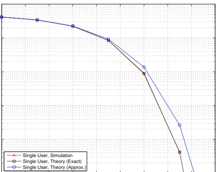
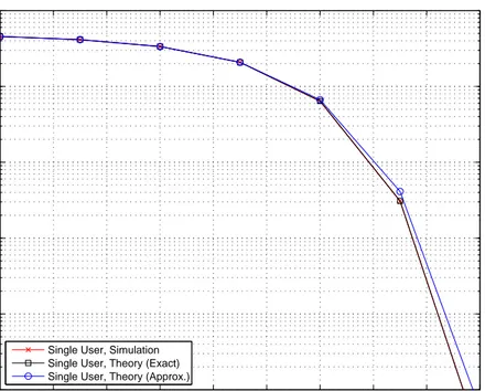
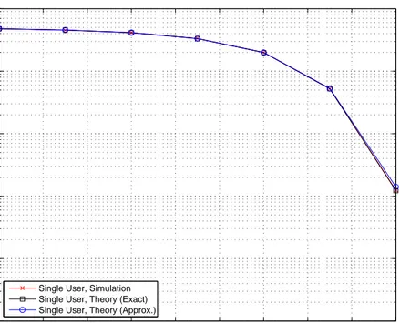
In order to compare the expressions in (2.33) and (2.38), some numerical evaluations are performed. Figures 2.1–2.5 plot the bit error probability (BEP)
versus the signal-to-noise ratio (SNR) for different numbers of frames Nf. From
the plots, it is observed that, for a constant symbol energy, the performance of the receiver degrades as Nf increases, which is expected from (2.38). Intuitively, the receiver collects more noise as Nf increases for a constant symbol energy. In addition, there is a good agreement between the exact theoretical results and the simulation results. However, the approximate theoretical results match closely
to the simulation results only for large values of Nf. This can be explained by
the fact that the Gaussian approximation assumes get accurate for large values of M Nf/2.
0 2 4 6 8 10 12 14 16 18 10−5 10−4 10−3 10−2 10−1 100 SNR (dB)
Bit Error Probability
Single User, Simulation Single User, Theory (Exact) Single User, Theory (Approx.)
Figure 2.1: BEP versus SNR for a single user system with Nf = 4 and E1 = 1.
0 2 4 6 8 10 12 14 16 18 10−5 10−4 10−3 10−2 10−1 100 SNR (dB)
Bit Error Probability
Single User, Simulation Single User, Theory (Exact) Single User, Theory (Approx.)
0 2 4 6 8 10 12 14 16 18 10−5 10−4 10−3 10−2 10−1 100 SNR (dB)
Bit Error Probability
Single User, Simulation Single User, Theory (Exact) Single User, Theory (Approx.)
Figure 2.3: BEP versus SNR for a single user system with Nf = 16 and E1 = 1.
0 2 4 6 8 10 12 14 16 18 10−5 10−4 10−3 10−2 10−1 100 SNR (dB)
Bit Error Probability
Single User, Simulation Single User, Theory (Exact) Single User, Theory (Approx.)
0 2 4 6 8 10 12 14 16 18 10−5 10−4 10−3 10−2 10−1 100 SNR (dB)
Bit Error Probability
Single User, Simulation Single User, Theory (Exact) Single User, Theory (Approx.)
Figure 2.5: BEP versus SNR for a single user system with Nf = 64 and E1 = 1.
In Figures 2.1–2.5, a single path channel is considered for simplicity, and the results are presented to verify the theoretical results (realistic multipath channels are considered in Chapter 4). Since a single path scenario is considered in the figures, the integration interval is taken as one pulse duration. Therefore, the degrees of freedom for the chi-square random variable in each frame is small since it is determined by the time duration and the bandwidth product. Therefore, the
Gaussian approximation gets accurate only for large Nf values since the degrees
of freedom of the decision variables are given by M Nf/2 as shown in (2.31) and
(2.32). In practical UWB channels, there can be a large number of multipath components; hence, a larger integration interval is employed. Therefore, the Gaussian approximation can get more accurate in practice.
2.3.3
Multiuser Case
In this section, the performance of the conventional receiver is analyzed for in multiuser environments. Although it is difficult to obtain a reasonable expression of the exact probability of error, a closed form expression can be obtained based on the Gaussian approximation as in [28].
Without loss of generality, user 1 is assumed as the user of interest in a K-user system. Assuming equiprobable information symbols for all users, the probability of error can be expressed as
Pe = 1 2K ∑ ˜ b∈{±1}K−1 ( P { D1− D2 ≥ 0 | b(1) =−1, ˜b } + P { D1 − D2 < 0| b(1) =−1, ˜b } ) , (2.39)
where ˜b = [b(2)· · · b(K)]T, and D1 and D2 are given as
D1 = ∑ j∈S χ2M(θj(b)) and D2 = ∑ j∈ ¯S χ2M(θj(b)) . (2.40)
Note that χ2M(θj(b)) is a noncentral chi-square random variable with M degrees
of freedom and a noncentrality parameter of θj(b). Here, M is the approximate
dimensionality of the signal space, which is obtained from the time-bandwidth
product, and θj(b) denotes the energy obtained from jth frame (in the absence
of noise) for information bits b = [b(1)· · · b(K)]T (see (2.21)).
In the following lemma, the asymptotical normality of D1 and D2 is shown
similarly to [28].
Lemma 2.2: As M Nf → ∞ , D1 and D2 are Gaussian distributed as
follows: D1 ∼ N ( ∑ j∈S (σ2M + θj(b)) , ∑ j∈S (2M σ4+ 4σ2θj(b)) ) , D2 ∼ N ∑ j∈ ¯S (σ2M + θj(b)) , ∑ j∈ ¯S (2M σ4+ 4σ2θj(b)) . (2.41)
Proof : Please see Appendix B.
Since |S| = | ¯S| = Nf/2, and the difference of two Gaussian random variables
is also Gaussian, the term D1− D2 is normally distributed as
D1− D2 ∼ N ∑ j∈S θj(b)− ∑ j∈ ¯S θj(b) , 2σ4M Nf + 4σ2 N∑f−1 j=0 θj(b) . (2.42)
Then, the probability of error can be calculated from (2.39) as
Pe = 1 2K ∑ ˜ b∈{±1}K−1 Q ∑ j∈ ¯S θj(˜b, b(1) =−1) − ∑ j∈S θj(˜b, b(1) =−1) √ 2σ4M N f + 4σ2 N∑f−1 j=0 θj(˜b, b(1) =−1) + Q ∑ j∈S θj(˜b, b(1) = 1)− ∑ j∈ ¯S θj(˜b, b(1) = 1) √ 2σ4M N f + 4σ2 N∑f−1 j=0 θj(˜b, b(1) = 1) (2.43)
Note that for the single user case; that is, b = b(1), the expression above reduces
Chapter 3
Optimal and Suboptimal
Receivers
In this chapter, some optimal and suboptimal receivers are studied for CM-TR UWB systems. First, low complexity receivers such as the blinking receiver (BR) and the chip discriminator are discussed (Section 3.1 and 3.2). The main idea behind these types of receivers is to discard some of the colliding pulses of the user of interest and to estimate the transmitted information symbol based on uncorrupted or slightly corrupted pulses. If the number of pulses with slight or no collision is sufficiently high per information symbol, these two receivers perform quite well. In addition to those receivers, a linear MMSE receiver is analyzed and discussed (Section 3.3). This MMSE receiver needs some partial channel knowledge and it is more complex than the previously discussed receivers. Lastly, the ML detector is investigated and its exact and approximate calculations are discussed (Section 3.4). Although, the ML detector is more complex and impractical in many cases, it is optimal and serves as a reference.
3.1
Blinking Receiver (BR)
The BR estimates the transmitted information symbol of the user of interest (user 1) based on the set of energy samples obtained from different frames with no collision of pulses [23]. In this case, the transmitted information symbol for user 1 can be estimated as follows:
∑ j∈S1 ˜ βjyj ∑ j∈S1 ˜ βj ˆb(1)=+1 > < ˆb(1)=−1 ∑ j∈ ¯S1 ˜ βjyj ∑ j∈ ¯S1 ˜ βj , (3.1)
where yj is the energy sample from the jth frame, S1 and ¯S1 are as in (2.8) and
(2.9), respectively, and the coefficients ˜βj are given by
˜ βj = 1 , if |c(1)j − c(k)j | ≥ Tds/Tc 0 , otherwise , (3.2)
with Tds denoting the delay spread of the channel and Tc being the chip interval. Note that this receiver requires the knowledge of collisions between the pulses of the user of interest and those of the interfering users. Therefore, this receiver is more complex than the conventional receiver. Note also that this receiver discards colliding pulses irrespective of the interference level. Thus, for channels with large delay spreads, this receiver may perform poorly. In the formulation, it is assumed that there occurs no inter-frame interference (IFI).
3.2
Chip Discriminator
In practice, there can be hundreds of echoes from multipath components and the channel delay spread can be significantly larger than the pulse duration in a UWB system. In such cases, the blinking receiver might be very inefficient, since it does not have any information about the energies of interferers. Instead, the chip discriminator can be considered. In the chip discriminator, the transmitted
information symbol for user 1 can be found as ∑ j∈S1 ˜ βjyj ∑ j∈S1 ˜ βj ˆb(1)=+1 > < ˆb(1)=−1 ∑ j∈ ¯S1 ˜ βjyj ∑ j∈ ¯S1 ˜ βj , (3.3)
where yj is the energy obtained from the jth frame and the coefficients ˜βj are
given by ˜ βj = 1 if |c(1)j − c(k)j | ≥ ∆c or AAk1 ≤ T 0 otherwise , (3.4)
where ∆c is the threshold for the difference between the time-hoping (TH) codes
of user-1 and user-k, and T is the threshold for the ratio between the amplitude of the kth user (Ak) and the user of interest (A1). By setting threshold values
T and ∆c, the colliding pulses with strong interferers are eliminated. In other words, the pulses with low levels of interference are taken into account as well.
It should be noted that depending on the number of frames (Nf), ∆c and T
values, the terms ∑j∈Sβ˜j or ∑
j∈ ¯Sβ˜j in (3.3) might be zero in some cases. In such scenarios, the conventional receiver ( ˜βj = 1, j = 0, . . . , Nf − 1) might be
used. Then, if the number of pulses per information symbol, Nf/2, is low, this
receiver might perform closely to the conventional receiver.
In order to implement this receiver, only TH sequences and symbol energies of all users are needed and two threshold levels must be determined. The per-formance of this detector can be improved by setting threshold T based on the interfering energy. However, this requires detailed channel information, hence, a more complex receiver structure.
In Table 3.1, the optimal threshold values are shown for an example two-user
scenario, in which the user energies are E1 = 1 and E2 = 2. The channel models
Table 3.1: Optimal threshold values for CM1, CM2, CM3 and CM4 channel
models in a 2-user system (E1 = 1 and E2 = 2) with Tc = 1 ns and SNR = 12
dB.
CM1 CM2 CM3 CM4
Optimal value of ∆c 25 25 12 20
3.3
Linear MMSE
In this section, the linear MMSE receiver is obtained. Let yj =
∫
Γj
r2(t)dt, j =
0, 1, . . . , Nf−1, represent the set of energy samples obtained from the Nf frames.
Assuming user 1 as the user of interest, yj can be expressed as
yj = ∫ Γj [r1(t) + rI(t) + n(t)] 2 dt = ∫ Γj [r1(t)]2dt + 2 ∫ Γj r1(t) [rI(t) + n(t)]2dt + ∫ Γj [rI(t) + n(t)]2dt , (3.5) where n(t) is the Gaussian noise and rI(t) is the sum of all interfering signals given by rI(t) = K ∑ k=2 rk(t) . (3.6)
The received signal from user-k during the jth frame can be expressed as
rjk(t) = √ Ek 2Nf a(k)j (1+b(k)d˜(k)j ) ˜w(t−jTf−c (k) j Tc) for t∈ [jTf, (j + 1)Tf) . (3.7)
From (3.7), (3.5) can be written as yj = E1 2Nf (2 + 2b(1)d˜(1)j ) ∫ Γj ˜ w2(t− jTf − c (1) j Tc)dt + 2 √ E1 2Nf a(1)j (1 + b(1)d˜(1)j ) ∫ Γj ˜ w(t− jTf − c (1) j Tc)[rI(t) + n(t)]dt + ∫ Γj [rI(t) + n(t)] 2 dt .
To simplify the notation, the expression above can be written as yj = E1γ (1) j Nf + b(1)αj+ nj , (3.8) where γj(1) = ∫ Γj ˜ w2(t− jTf − c (1) j Tc)dt (3.9) αj = E1γj(1) Nf ˜ d(1)j + √ 2E1 Nf a(1)j d˜(1)j ∫ Γj ˜ w(t− jTf − c (1) j Tc)[rI(t) + n(t)]dt (3.10) nj = √ 2E1 Nf a(1)j ∫ Γj ˜ w(t− jTf − c (1) j Tc)[rI(t) + n(t)]dt + ∫ Γj [rI(t) + n(t)]2dt . (3.11) It should be noted that γj(1) = Ew˜ if Γj includes all the multipaths.
Considering all the frames from 0 to Nf − 1, (3.8) can be generalized as
y = k + b(1)α + n , (3.12) where k, E1 Nf [ γ0(1)· · · γN(1) f−1 ]T (3.13) α, [α0· · · αNf−1] T (3.14) n , [n0· · · nNf−1] T . (3.15)
In the linear MMSE receiver, the information symbol is estimated as [30] ˆb(1) = sgn{θT
MMSEy
}
where
θMMSE = arg min
θ E {( θTy− b(1))2 } =(E{yyT})−1E{α} =(kkT + E{n} kT + kE{nT}+ E{ααT}+ E{nnT})−1E{α} . (3.17) The closed-form expressions for the terms in (3.17) are obtained in the following lemmas.
Lemma 3.1: Let the polarity randomization codes, a(k)j , k = 2, . . . , K be i.i.d. random variables that take values ±1 with equal probability. Then, E {nj} can be obtained as E{nj} = K ∑ k=2 Ek Nf χj,k+|Γj| 2Bσ2 , (3.18)
where |Γj| denotes the length of the integration interval in the jth frame, and χj,k , ∫ Γj [ ˜ w ( t− jTf − c(k)j Tc )]2 dt . (3.19)
Proof : Please see Appendix C.
Lemma 3.2: Let the polarity randomization codes, a(k)j , k = 2, . . . , K be i.i.d. random variables that take values±1 with equal probability. Then, E {njnl} can be expressed as E{njnl} = 4B2σ4|Γ|2 ( 1 + B1|Γ| ) + K ∑ k=2 E2 k N2 f ( 1 + d(k)j d(k)l ) χj,k1χl,k2 +2Bσ2|Γ|∑K k=2 Ek Nf (χj,k+ χl,k) + ∑ k1̸=k2 Ek1Ek2 N2 f χj,k1χl,k2 , j ̸= l 4B2σ4|Γ|2( 1 + 1 B|Γ| ) + K ∑ k=2 2E2 k N2 f (χj,k)2+ 4σ2 K ∑ k=2 Ek Nf (B|Γ| + 1) χj,k + ∑ k1̸=k2 Ek1Ek2 N2 f ( χj,k1χj,k2 + 2 [ Rjw˜((c(k1) j − c (k2) j )Tc) ]2) +2E1 Nf [∑K k=2 Ek Nf [ Rwj˜((c(1)j − c(k)j )Tc) ]2 + σ2γ(1) j ] , j = l (3.20)
where |Γ| denotes the common integration interval for all the frames.
Proof : Please see Appendix D.
Lemma 3.3: Let the polarity randomization codes, a(k)j , k = 2, . . . , K be i.i.d. random variables that take value ±1 with equal probability. Then, E {αjαl} can be found as E{αjαl} = E2 1 N2 f γj(1)γl(1)d(1)j d(1)l , j ̸= l E2 1 N2 f (χj,k) 2 +2E1 Nf [∑K k=2 Ek Nf [ Rwj˜((c(1)j − c(k)j )Tc) ]2 + σ2γ(1) j ] , j = l (3.21)
Proof : Please see Appendix E.
Note that E{yyT}in (3.17) can be estimated from the previous observations
in practice. Also, for polarity randomization codes a(k)j ∈ {−1, +1} being equally likely, E{αj} = E1γ (1) j Nf ˜ d(1)j , (3.22)
where γj(1) is given in (3.9). Thus, in order to implement this MMSE receiver,
the symbol energy, the TH sequence and the orthogonalization codes of the user
of interest (user 1) and γj(1) must be known. Moreover, the implementation of
this receiver requires a matrix inversion. Therefore, the MMSE receiver is more complex than the BR, the chip discriminator, and the conventional receiver.
Note also that the information symbol can be estimated based on Lemmas 3.1–3.3 for the theoretical evaluation of the MMSE receiver. In this case, the knowledge of the symbol energies, the TH sequences and the orthogonalization codes for all users is required. In addition, the channel state information, the bandwidth of the receive filter and the integration interval should be known for those theoretical evaluations.
3.4
Maximum-Likelihood (ML) Detector
In order to compare the receivers discussed previously, the maximum-likelihood (ML) detector is chosen as a reference. This receiver might be considered as
impractical, since it searches over 2K hypotheses. However, it minimizes the
probability of error and serves as an optimal receiver. In the ML detector, the set of information symbols b = [b(1)...b(K)]T is estimated as
ˆ
b = arg max
b pb(y) = arg maxb
N∏f−1
j=0
pb(yj) . (3.23)
Taking the logarithm, we obtain ˆ
b = arg max
b log (pb(y)) = arg maxb
N∑f−1
j=0
log (pb(yj)) , (3.24)
where pb(yj) is non-central chi-square distributed and given by
pb(yj) = 1 2σ2 ( yj θj(b) )M 4− 1 2 e− (θj (b)+yj) 2σ2 IM 2−1 (√ θj(b)yj σ2 ) . (3.25)
Note that, for a given set of binary information symbols b, if the signal energy (in the absence of noise) is zero; that is, θj(b) = 0, then yj is central chi-square distributed and pb(yj) given above reduces to
pb(yj) = y M 2 −1 j e yj 2σ2 σM2m2Γ(M/2) . (3.26)
From (3.25), (3.24) can be expressed as
arg max b N∑f−1 j=0 ( M 4 − 1 2 ) [log yj − log (θj(b))] − (θj(b) + yj) 2σ2 + log { IM 2−1 (√ θj(b)yj σ2 )} . (3.27)
The expression in (3.27) provides an exact expression for the ML detector. How-ever, the objective function can be computationally complex to evaluate. There-fore, the Gaussian approximation is used to provide a simpler alternative solution.
In Chapter 2, it has been observed that the Gaussian approximation can be
employed for large values of M . Hence, the PDF of yj can be written as
pb(yj) = 1 √ 2πσj e− (yj −µj )2 2σ2j , (3.28)
where µj and σj are given respectively by
µj = σ2M + θj(b) , (3.29)
σj = 2M σ4+ 4σ2θj(b) . (3.30)
Thus, (3.24) can be expressed alternatively as
arg max
b log (pb(y)) = arg maxb
N∑f−1 j=0 log (pb(yj)) = arg min b N∑f−1 j=0 { log(√2πσj) + (yj − µj)2 2σ2 j } . (3.31)
Note that in order to implement this detector, the channel state information, the TH sequences, the polarity and orthogonalization codes for all users must be known. This ML receiver is the most complex receiver among all the receivers discussed in this study and serves as a reference.
As a special case, the ML detector can be investigated in a single user scenario. In this case, (3.24) reduces to the Bayes decision rule, which, for equiprobable information symbols and uniform cost assignment, can be expressed as [1]
∏ j∈S y 1 2− M 4 j IM2−1 (√ θyj σ2 )ˆb=+1 > < ˆ b=−1 ∏ j∈ ¯S y 1 2− M 4 j IM2−1 (√ θyj σ2 ) . (3.32)
Note that the Bayes rule in (3.32) also gives the minimum probability of error due to the assumption of uniform cost assignment [31]. In [1], it is shown that for large M values, the conventional receiver has nearly the same performance as the optimal receiver in (3.32). As an example, Figure 3.1 plots the BEP versus M for the conventional and the optimal receivers. From the plot, it is observed that
degrees of freedom parameter, M , is determined by the product of the bandwidth
and integration interval (Γj). In practice, due to a large number of multipath
components, B|Γj| ≫ 1 and the condition of M ≥ 8 is commonly satisfied.
1 2 3 4 5 6 7 8 9 10−6 10−5 10−4 10−3 10−2 10−1 100 log2M BER Conventional Optimal θ = 10 N f = 10 θ = 25 Nf = 4
Figure 3.1: BEP versus M for the conventional and the optimal receivers for the single user scenario [1].
Chapter 4
Simulation Studies
In this chapter, simulation results are presented in order to verify the theoretical results and to compare the performance of the receivers considered in the previous chapters. The UWB pulse w(t) is chosen as the second order derivative of the Gaussian pulse [32]; that is,
w(t) = ( 1− 4πt 2 ζ2 ) e− 2πt2 ζ2 /√E p , (4.1)
where Ep is a scalar chosen to set w(t) to unit energy and ζ = Tc/2.5 determines
the pulse width. An example of a unit energy pulse with Tc = 1 ns is illustrated
in Figure 4.1. The bandwidth of the receive filter is 5 GHz and the channel statistics are taken from the IEEE 802.15.4a models CM1, CM2, CM3 and CM4 [29]. For the considered CM-TR UWB system, the system parameters are chosen
as Nf = 4 and Nc = 250, which correspond to a data rate of Rb = 1 Mbit/s data
rate.
In order to prevent catastrophic collisions between pulses of different users,
TH sequences are employed for each user in each case. To avoid
inter-frame interference (IFI), the TH sequences are chosen uniformly from the set {0, 1, . . . , Nc− Nw}, where Nw = ⌈ Tw(i) Tc ⌉ , (4.2)
with Tw(i) being the duration of channel response to the pulse given in 4.1 for the ith channel model, Tc is chip duration (equal to 1 ns in the simulations) and ⌈·⌉ is the ceiling function. Table 4.1 indicates the values of Nw for different channel models and the sets from which the TH sequences are chosen to avoid IFI.
Table 4.1: TH sequence sets for CM1, CM2, CM3 and CM4 channel models. Channel Model Nw TH set CM1 120 c(k)j ∈ {0, 1, . . . , 130} CM2 140 c(k)j ∈ {0, 1, . . . , 110} CM3 90 c(k)j ∈ {0, 1, . . . , 160} CM4 80 c(k)j ∈ {0, 1, . . . , 170} −0.5 −0.4 −0.3 −0.2 −0.1 0 0.1 0.2 0.3 0.4 0.5 −1.5 −1 −0.5 0 0.5 1 1.5 2 2.5 3x 10 4 Time (ns) Amplitude
Due to the highly dispersive channel responses, the duration of the
inte-gration interval |Γ| is critical and can affect the performance of the receivers
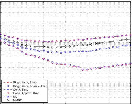
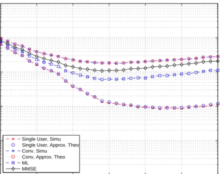
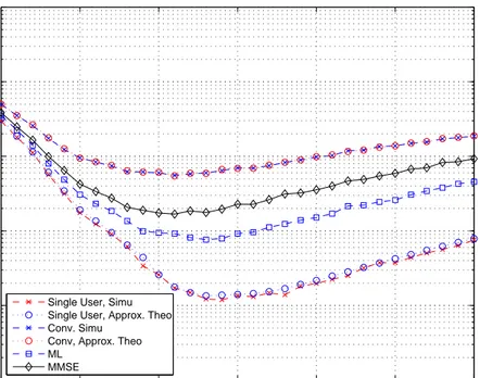
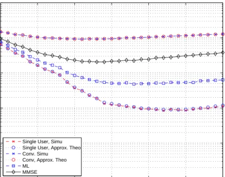
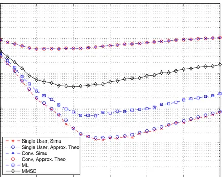
significantly1. Figures 4.2–4.5 plot the BEP versus the integration interval |Γ|
for a two-user system for channel models CM1, CM2, CM3, and CM4, respec-tively. The integration intervals for the minimum probability of error is given in Table 4.2. From the plots and the table, it is observed that the performances
of receivers are highly dependent on the integration interval |Γ| and its optimal
value is different for different receivers. Figures 4.6–4.9 plot the BEP versus the integration interval Γ, where the symbol energy of the interfering user is equal to 2. The integration intervals for the minimum probability of error are given in Table 4.3. 10 20 30 40 50 60 70 10−5 10−4 10−3 10−2 10−1 100 Integration interval (ns)
Bit Error Probability
Single User, Simu Single User, Approx. Theo Conv. Simu
Conv, Approx. Theo ML
MMSE
Figure 4.2: BEP versus |Γ| for a 2-user system for CM1 with Nf = 4, Nc = 250
and Ek = 1 for k = 1, 2.
10 20 30 40 50 60 70 10−5 10−4 10−3 10−2 10−1 100 Integration interval (ns)
Bit Error Probability
Single User, Simu Single User, Approx. Theo Conv. Simu
Conv, Approx. Theo ML
MMSE
Figure 4.3: BEP versus |Γ| for a 2-user system for CM2 with Nf = 4, Nc = 250
and Ek = 1 for k = 1, 2. 10 20 30 40 50 60 70 10−5 10−4 10−3 10−2 10−1 100 Integration interval (ns)
Bit Error Probability
Single User, Simu Single User, Approx. Theo Conv. Simu
Conv, Approx. Theo ML
MMSE
Figure 4.4: BEP versus |Γ| for a 2-user system for CM3 with Nf = 4, Nc = 250
10 20 30 40 50 60 70 10−5 10−4 10−3 10−2 10−1 100 Integration interval (ns)
Bit Error Probability
Single User, Simu Single User, Approx. Theo Conv. Simu
Conv, Approx. Theo ML
MMSE
Figure 4.5: BEP versus |Γ| for a 2-user system for CM4 with Nf = 4, Nc = 250
and Ek = 1 for k = 1, 2. 10 20 30 40 50 60 70 10−5 10−4 10−3 10−2 10−1 100 Integration interval (ns)
Bit Error Probability
Single User, Simu Single User, Approx. Theo Conv. Simu
Conv, Approx. Theo ML
MMSE
Figure 4.6: BEP versus |Γ| for a 2-user system for CM1 with Nf = 4, Nc = 250,
10 20 30 40 50 60 70 10−5 10−4 10−3 10−2 10−1 100 Integration interval (ns)
Bit Error Probability
Single User, Simu Single User, Approx. Theo Conv. Simu
Conv, Approx. Theo ML
MMSE
Figure 4.7: BEP versus |Γ| for a 2-user system for CM2 with Nf = 4, Nc = 250,
E1 = 1 and E2 = 2. 10 20 30 40 50 60 70 10−5 10−4 10−3 10−2 10−1 100 Integration interval (ns)
Bit Error Probability
Single User, Simu Single User, Approx. Theo Conv. Simu
Conv, Approx. Theo ML
MMSE
Figure 4.8: BEP versus |Γ| for a 2-user system for CM3 with Nf = 4, Nc = 250,
10 20 30 40 50 60 70 10−5 10−4 10−3 10−2 10−1 100 Integration interval (ns)
Bit Error Probability
Single User, Simu Single User, Approx. Theo Conv. Simu
Conv, Approx. Theo ML
MMSE
Figure 4.9: BEP versus |Γ| for a 2-user system for CM4 with Nf = 4, Nc = 250,
E1 = 1 and E2 = 2.
Table 4.2: Optimal integration intervals for CM1, CM2, CM3 and CM4 channel
models in a 2-user system (Ek = 1, for k = 1, 2) with 12 dB SNR value. All the
quantities are in nanosecond (ns). Channel Model Single User, Simu. Single User, Theo. Conv. Rec., Simu. Conv. Rec., Theo. MMSE Re-ceiver ML Detec-tor CM1 48 48 32 32 38 32 CM2 54 54 42 42 38 38 CM3 22 22 18 18 18 18 CM4 36 36 32 32 32 36
Table 4.3: Optimal integration intervals for CM1, CM2, CM3 and CM4 channel
models in a 2-user system (E1 = 1 and E2 = 2) with 12 dB SNR value. All the
quantities are in nanosecond (ns). Channel Model Single User, Simu. Single User, Theo. Conv. Rec., Simu. Conv. Rec., Theo. MMSE Re-ceiver ML Detec-tor CM1 48 48 18 18 26 48 CM2 54 54 32 32 36 46 CM3 22 22 10 10 18 22 CM4 36 36 20 20 30 36 −5 0 5 10 15 20 10−5 10−4 10−3 10−2 10−1 100 Eh/No (dB)
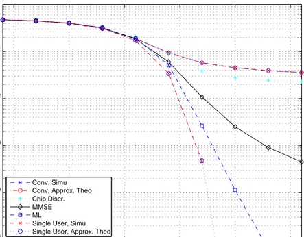
Bit Error Probability
Conv. Simu Conv, Approx. Theo Chip Discr. MMSE ML
Single User, Simu Single User, Approx. Theo
Figure 4.10: BEP versus Eh/N0 for a 2-user system for CM1 with Nf = 4,
−5 0 5 10 15 20 10−5 10−4 10−3 10−2 10−1 100 Eh/No (dB)
Bit Error Probability
Conv. Simu Conv, Approx. Theo Chip Discr. MMSE ML
Single User, Simu Single User, Approx. Theo
Figure 4.11: BEP versus Eh/N0 for a 2-user system for CM1 with Nf = 4,
Nc = 250, E1 = 1 and E2 = 2. −5 0 5 10 15 20 10−5 10−4 10−3 10−2 10−1 100 Eh/No (dB)
Bit Error Probability
Conv. Simu Conv, Approx. Theo Chip Discr. MMSE ML
Single User, Simu Single User, Approx. Theo
Figure 4.12: BEP versus Eh/N0 for a 2-user system for CM2 with Nf = 4,
−5 0 5 10 15 20 10−5 10−4 10−3 10−2 10−1 100 Eh/No (dB)
Bit Error Probability
Conv. Simu Conv, Approx. Theo Chip Discr. MMSE ML
Single User, Simu Single User, Approx. Theo
Figure 4.13: BEP versus Eh/N0 for a 2-user system for CM2 with Nf = 4,
Nc = 250, E1 = 1 and E2 = 2. −5 0 5 10 15 20 10−5 10−4 10−3 10−2 10−1 100 Eh/No (dB)
Bit Error Probability
Conv. Simu Conv, Approx. Theo Chip Discr. MMSE ML
Single User, Simu Single User, Approx. Theo
Figure 4.14: BEP versus Eh/N0 for a 2-user system for CM3 with Nf = 4,
−5 0 5 10 15 20 10−5 10−4 10−3 10−2 10−1 100 Eh/No (dB)
Bit Error Probability
Conv. Simu Conv, Approx. Theo Chip Discr. MMSE ML
Single User, Simu Single User, Approx. Theo
Figure 4.15: BEP versus Eh/N0 for a 2-user system for CM3 with Nf = 4,
Nc = 250, E1 = 1 and E2 = 2. −5 0 5 10 15 20 10−5 10−4 10−3 10−2 10−1 100 Eh/No (dB)
Bit Error Probability
Conv. Simu Conv, Approx. Theo Chip Discr. MMSE ML
Single User, Simu Single User, Approx. Theo
Figure 4.16: BEP versus Eh/N0 for a 2-user system for CM4 with Nf = 4,
![Figure 3.1: BEP versus M for the conventional and the optimal receivers for the single user scenario [1].](https://thumb-eu.123doks.com/thumbv2/9libnet/5986779.125626/43.892.279.700.278.608/figure-bep-versus-conventional-optimal-receivers-single-scenario.webp)