Modelling and robust controller design for a multi-axis micro-milling machine

MODELLING AND ROBUST CONTROLLER

DESIGN FOR A MULTI-AXIS

MICRO-MILLING MACHINE

a thesis submitted to

the graduate school of engineering and science

of bilkent university

in partial fulfillment of the requirements for

the degree of

master of science

in

mechanical engineering

By

M¨

umtazcan Karag¨

oz

September 2016

MODELLING AND ROBUST CONTROLLER DESIGN FOR A MULTI-AXIS MICRO-MILLING MACHINE

By M¨umtazcan Karag¨oz

September 2016

We certify that we have read this thesis and that in our opinion it is fully adequate, in scope and in quality, as a thesis for the degree of Master of Science.

Melih C¸ akmakcı(Advisor)

Yi˘git Karpat

Ulu¸c Saranlı

Approved for the Graduate School of Engineering and Science:

Levent Onural

ABSTRACT

MODELLING AND ROBUST CONTROLLER DESIGN

FOR A MULTI-AXIS MICRO-MILLING MACHINE

M¨umtazcan Karag¨oz

M.S. in Mechanical Engineering

Advisor: Melih C¸ akmakcı

September 2016

In the current era of miniaturization, micro manufacturing had became one of the most popular topics. Even tough there are new promising methods such as laser sintering and 3D printing; conventional manufacturing methods continue to hold a unique and irreplaceable position. This thesis aims to design a robust con-trol algorithm for a three axis micro-machining system. In order to synthesize the controller, first the system is modeled. After the modeling, a system identification due to non-linearities is also performed. X, Y and Z axis’s identified using pre-pared Sum of sines identification input. Verification data shows these identified transfer functions represent the physical system well while avoiding over-fit.

Us-ing these identified transfer functions, a robust H∞ controller is synthesized with

designed weighting functions. In simulations, this robust H∞ controller showed

significantly better performance with or without disturbance. Machining experi-ments are also done in order to compare the performance of robust controller with the PID controller. According to results of experiments, robust controller showed similar tracking performance with improved surface quality and less oscillations vibrations.

¨

OZET

¨

UC

¸ BOYUTLU M˙IKRO ˙IS

¸LEME C˙IHAZI

MODELLENMES˙I VE G ¨

URB ¨

UZ KONTROLC ¨

U

TASARIMI

M¨umtazcan Karag¨oz

Makine M¨uhendisli˘gi, Y¨uksek Lisans

Tez Danı¸smanı: Melih C¸ akmakcı

Eyl¨ul 2015

˙I¸cinde bulundu˘gumuz bu minyat¨urle¸sme ¸ca˘gında, mikro ¨uretim en pop¨uler ara¸stırma konularından biri haline gelmi¸stir. Her ne kadar 3 Boyutlu yazıcılar

ve laser sinterleme gibi yeni ¨uretim teknolojileri gelecek vaat ediyor olsa da,

con-vensiyonel ¨uretim teknolojileri hala yeri doldurulamaz bir pozisyondadır. Bu tez

¨

u¸c boyutlu bir mikro i¸sleme sistemi i¸cin g¨urb¨uz bir kontrolc¨u tasarlamayı

hede-flemektedir. Kontrolc¨un¨un sentezlenmesi i¸cin ilk olarak sistem modellenmi¸stir.

Ancak daha sonra sistem modelinin, sistem tanılama metodu ile elde edilmesi

kararla¸stırılmı¸stır. X, Y ve Z eksenlerinin transfer fonksiyonları, sin¨usler toplamı

girdisi kullanılarak hesaplanmı¸stır. Do˘grulama deneylerinin sonu¸clarına g¨ore elde

edilen transfer fonksiyonları sistemi yansıtmaktadır. Elde edilen bu transfer

fonksiyonları ve tasarlanan a˘gırlık fonksiyonlarının yardımı ile g¨urb¨uz bir H∞

kon-trolc¨u tasarlanmı¸stır. Simulasyon ¸cıktılarına g¨ore tasarlanan bu g¨urb¨uz kontrolc¨u

hem disturbans girdisi varken hem de yokken PID kontrolc¨us¨une g¨ore belirgin bir

¸sekilde daha iyi performans g¨ostermi¸stir. Son b¨ol¨umde tasarlanan bu g¨urb¨uz

kon-tolc¨u ile PID kontrolc¨us¨u kesme testlerinde kar¸sıla¸stırılmı¸stır. Bu testlere g¨ore,

PID kontrolc¨us¨u ve g¨urb¨uz kontrolc¨u benzer bir izleme performansı g¨osterse de,

g¨urb¨uz kontrolc¨u ile daha iyi bir y¨uzey kalitesi elde edilebilirken aynı zamanda

¨

uretim sırasında daha az titre¸sim olu¸smaktadır.

Acknowledgement

First of all, I would like to thank my thesis advisor Prof. Melih C¸ akmakcı for his

motivation, patience, enthusiasm, and immense knowledge. His guidance helped me in all the time of research and writing of this thesis. I could not have imagined having a better advisor and mentor for my study.

I also thank my fellow office mates Serhat Kerimo˘glu, Bu˘gra T¨ureyen, Atakan

Arı and Alper Tiftik¸ci for priceless companion and all the fun we have had in the last three years.

Also, I thank my elder brother Korhan Karag¨oz for his endless support and being

there for me anytime and everytime.

Finally, I must express my very profound gratitude to my parents Vedat and

Pervin Karag¨oz for providing me with limitless support and continuous

encour-agement throughout my study and through the process of researching and writing this thesis.

This accomplishment would not have been possible without all of you. Thank you.

Contents

1 Introduction 1

2 System Modeling and System Identification 4

2.1 Mathematical Modeling . . . 4

2.2 System Identification . . . 5

2.2.1 Identification Inputs . . . 6

2.2.2 Identified Transfer Functions . . . 10

3 Robust Controller Synthesis 21 3.1 H∞ Problem . . . 21

3.2 Loop Shaping . . . 22

3.3 H∞ Controller Synthesis For Micro-Machining System . . . 22

3.3.1 Weighting Functions . . . 23

3.3.2 Synthesized Robust Controllers . . . 28

CONTENTS vii

3.4.1 Simulation Design . . . 29

3.4.2 Simulation Results- Without Disturbance . . . 31

3.4.3 Simulation Results - With Disturbance . . . 41

4 Micro-machining Experiments 48 4.1 PID with CCC Controller . . . 49

4.1.1 Circular Cutting Test . . . 49

4.1.2 Square Cutting Test . . . 53

4.2 Robust Controller . . . 57

4.2.1 Circular Cutting Test . . . 57

4.2.2 Square Cutting Test . . . 58

5 Conclusion 59

List of Figures

2.1 Model of a Individual Axis . . . 5

2.2 Identification Input of X axis in Time Domain . . . 7

2.3 Verification Input of X axis in Time Domain . . . 7

2.4 Identification Input of X axis in Time Domain . . . 8

2.5 Verification Input of X axis in Time Domain . . . 8

2.6 Identification Input of X axis in Time Domain . . . 9

2.7 Verification Input of X axis in Time Domain . . . 9

2.8 Measured vs Simulated Response in Frequency Domain: X axis . 11 2.9 Measured vs Simulated Verification Response in Frequency Do-main: X axis . . . 11

2.10 Measured vs Simulated Response: X axis . . . 12

2.11 Measured vs Simulated Verification Response: X axis . . . 13

LIST OF FIGURES ix

2.13 Measured vs Simulated Verification Response in Frequency

Do-main: Y axis . . . 15

2.14 Measured vs Simulated Response in Time Domain: Y axis . . . . 16

2.15 Measured vs Simulated Verification Response in Time Domain: Y axis . . . 16

2.16 Measured vs Simulated Response in Frequency Domain: Z axis . . 18

2.17 Measured vs Simulated Verification Response in Frequency Do-main: Z axis . . . 19

2.18 Measured vs Simulated Response in Time Domain: Z axis . . . . 20

2.19 Measured vs Simulated Verification Response in Time Domain: Z axis . . . 20

3.1 General Control Problem Structure for H∞. . . 21

3.2 Weight Function: Ws of X Axis . . . 24

3.3 Weight Function: Wt of X Axis . . . 24

3.4 Weight Function: Ws of Y Axis . . . 25

3.5 Weight Function: Wt of Y Axis . . . 26

3.6 Weight Function: Ws of Z Axis . . . 27

3.7 Weight Function: Wt of Z Axis . . . 27

3.8 Simulation Setup With PID Controller . . . 29

LIST OF FIGURES x

3.10 Geometric Relations Of Contour Error . . . 31

3.11 Desired Output . . . 32

3.12 Desired Output vs Simulation Output with PID Controller: X vs Y 33 3.13 Desired Output vs Simulation Output with PID Controller: Y vs Z 33 3.14 Error vs Time with PID Controller: X axis . . . 34

3.15 Error vs Time with PID Controller: Y axis . . . 34

3.16 Error vs Time with PID Controller: Z axis . . . 35

3.17 Desired Output vs Simulation Output with Robust Controller: X vs Y . . . 37

3.18 Desired Output vs Simulation Output with Robust Controller: Y vs Z . . . 38

3.19 Error vs Time with Robust Controller: X axis . . . 39

3.20 Error vs Time with Robust Controller: Y axis . . . 39

3.21 Error vs Time with Robust Controller: Z axis . . . 40

3.22 Error vs Time with PID Controller: X axis . . . 42

3.23 Error vs Time with PID Controller: Y axis . . . 42

3.24 Error vs Time with PID Controller: Z axis . . . 43

3.25 Error vs Time with Robust Controller: X axis . . . 45

3.26 Error vs Time with Robust Controller: Y axis . . . 45

LIST OF FIGURES xi

4.1 Micro-Machining System . . . 49

4.2 Input Signal: Z vs Y axis . . . 50

4.3 Input Signal: Y vs Time . . . 51

4.4 Input Signal: Z vs Time . . . 51

4.5 Input Signal: X vs Time . . . 52

4.6 Optical Microscope Image Of the Circular Cut . . . 52

4.7 Input Signal: Z vs Y axis . . . 53

4.8 Input Signal: Y vs Time . . . 54

4.9 Input Signal: Z vs Time . . . 55

4.10 Input Signal: X vs Time . . . 55

4.11 Input Signal: X vs Time . . . 56

4.12 Optical Microscope Image Of the Square Cut . . . 56

4.13 Optical Microscope Image Of the Circular Cut . . . 57

List of Tables

2.1 Poles and Zeros: Gxx . . . 12

2.2 Poles and Zeros: Gyy . . . 17

2.3 Poles and Zeros: Gzz . . . 20

3.1 PID Parameters . . . 32

3.2 Rms Errors: PID Controller . . . 36

3.3 Rms Errors: Robust Controller . . . 41

3.4 Rms Errors with Disturbance Input: PID Controller . . . 44

Chapter 1

Introduction

Starting from the early 1960’s by the efforts of Feynman[1], the most prominent trend in manufacturing and engineering in the search of more efficent, more pow-erful and less cost devices is the miniaturization.[2] In the current era of miniatur-ization, micro manufacturing had became one of the most popular topics. Even tough there are new promising methods such as laser sintering and 3D printing; conventional manufacturing methods continue to hold a unique and irreplaceable position. The aim of this thesis is to design a robust control algorithm for a three axis micromachining system. In order to successfully manufacture micro scaled parts, the micromachining system need to be both precise and robust. Precision requirement emerges because of the nature of micro manufacturing ; furthermore robustness is required because of the nonlinear cutting forces [3], possibility of chatter vibration and other environmental disturbances such as electrical noise and ground vibration. The motivation of this thesis, is to design a robust mod-ular controller algorithm which satisfy the performance metrics and compare its operation to conventional controllers such as a CC PID controller.

In literature, there are studies and applications of different robust controller algo-rithms such as µ synthesis or ARC to the manufacturing systems such as milling machines.

Stephans and Knospe showed that µ synthesis could be used in order to synthesize a robust controller for machining spindles. [4]. It shown that, the robust controller synthesized using µ synthesis could result in an improved cutting performance while reducing chatter vibration. But it must be noted that, high order models used in the modeling of the spindle result in a high order robust controller (>50). Lee and Tomizuka showed that robust controllers could be used in high accuracy motion positioning systems. [5] The proposed controller have 4 components, a friction compensator either in the feedforward or feedback loop, a disturbance observer in the velocity loop, a feedback controller in the position loop, and a feedforward controller. It is shown that the controller has better performance compared to other digital controllers such as; ZP or ZPFC controllers.

Kashani et. al showed that H∞synthesis could be used in machining and turning

processes to increase surface texture.[6] Using the modeled dynamics of a turning process and simulations using MATLAB and SIMULINK, Kashani et. al. showed that active vibration control could result in a major improvement to the surface texture.

Tsao and Tsu-Chin showed that robust adaptive controllers could be used for non-circular machining.[7] Firstly, a system identification is carried for hydraulic servos. Then a robust adaptive repetitive controller is designed and implemented. Yao et al. showed that using an ARC (adaptive robust controller), friction mod-eling could be eliminated since the controller can cope with larger parameter variance.[8] Moreover, it is shown that resulting controller is considerably simpler and have a better tracking performance compared to the conventional controllers. Also, control saturation is avoided because of the built in anti-windup properties of ARC.

Moradi et al. showed that using H∞ controller, chatter vibration can be

sig-nificantly reduced. [9] Moreover it is shown that, as the parameter variance in-creases the effort needed to supress the chatter vibration is also inin-creases. Also, the difference between the actual system and modeled system greatly effects the

performance of the robust controller.

This thesis includes, system modeling, the system identification, robust controller synthesis and the cutting experiments of the system using the synthesized robust controller.

One of the key points of the controller design is the correct mathematical repre-sentation of the system. In this thesis, first the system modeling is carried out, but then it is decided to carry out a system identification procedure to represent the system mathematically better while avoiding over complexity. The procedure

of the system identification is explained in the 2nd chapter throughly.

In chapter 3, a robust controller is synthesized using the identified transfer func-tions. The synthesis of the robust controller requires design of weight functions, which effect the closed loop system dynamics dramatically. Then, synthesized robust controller is simulated using SIMULINK software and compared to the conventional PID controller.

Finally in chapter 5, the cutting tests performed by PID and Robust controllers. The performance of the two controllers are compared using the optical microscope images of the manufactured parts.

Chapter 2

System Modeling and System

Identification

In order to synthesize the robust controller, first the system must be mathe-matically represented. In the following section the modeling of the system is explained.

2.1

Mathematical Modeling

First approach to modeling of the system is to model the system as a 3 separate, identical single axis subsystems. Each of these single axis subsystems can be modeled as a linear DC motor system.

Using the model transfer function is calculated as: X(s) E(s) = kf LmS3_{+ (Rm + bL)s}2_{+ (Rb + k} bkf)s (2.1)

Even tough this model could be used to calculate a robust controller there are several problems regarding the model. First of all, this model uses a Coloumb friction model whereas the micro-machining system shows stick-slip behavior.

Figure 2.1: Model of a Individual Axis

Moreover, usage of a more advanced friction model may end up in a complex system model. Secondly, this model assumes that X, Y and Z axis are identical and have exactly the same transfer functions, which is not the actual case ac-cording to the identification results. Lastly, un-modeled dynamics could have a significant effect on the system response. So because of that reasons, it is decided to conduct a system identification procedure to achieve a better system model.

2.2

System Identification

System Identification is the procedure of measuring input and output data of any given system and using this input-output data to calculate a system model corresponding to the actual response of the system. Moreover, one must carefully select the identification input since both it need to be complex enough to extract meaningful information(persistent excitation) and also band-limited to the sam-pling frequency of the system. Furthermore, the identified system needs to be fit closely to the actual system while avoiding over-fit.

The measurement for the system identification tests are taken by using Heiden-hain LIP481R linear optical encoders with adaptive correction and look-up table based interpolation method. Ulu et al. showed that using that method and Heidenhain LIP481R linear optical encoders resolutions as high as 10nm can be achieved. [10]

Three axis’s of the system (X,Y and Z) excited by the identification input sepa-rately, gathering X,Y and Z data. As a result, the transfer function matrix could be calculated from this data. But it is seen that cross effect between the axis’s are extremely small which can safely omitted. For each data set, (identification and verification data sets) the identification tests repeated 5 times with different starting points. In transfer function identification and verification, the averaged data of these repetitions is used.

2.2.1

Identification Inputs

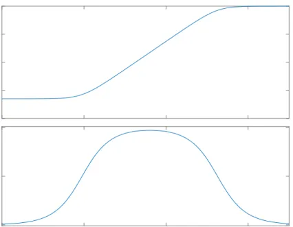
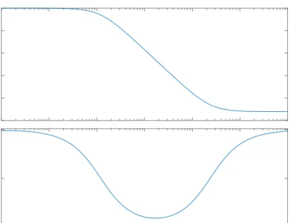
There are several options for system identification inputs such as sweep, random or sum of harmonic signals. Each of these inputs have their own advantages. For this application, sum of sines input is selected. Because, sweep signal is not feasible since the working range of the system is limited and system tends to drift because of the stick-slip friction, random signal is not feasible since each of the axis’s are identified individually therefore repeatability is an important factor. As it can be seen from the figures below, the identification input is selected as sum of sines with different frequency’s. As a result, the final identification signal is a highly complicated periodical signal in time domain.

For verification purposes, a signal with the same frequency content but with a different magnitude is used. The transfer functions calculated from the input signal data is compared to the verification signal data. The identification and verification signals used for each axis is given below.

2.2.1.1 X axis 0 5 10 15 20 25 30 Time(s) -0.8 -0.6 -0.4 -0.2 0 0.2 0.4 0.6 0.8 Amplitude

Figure 2.2: Identification Input of X axis in Time Domain

0 5 10 15 20 25 30 Time(s) -0.8 -0.6 -0.4 -0.2 0 0.2 0.4 0.6 0.8 Amplitude

2.2.1.2 Y axis 0 2 4 6 8 10 12 14 Time(s) -0.6 -0.4 -0.2 0 0.2 0.4 Amplitude

Figure 2.4: Identification Input of X axis in Time Domain

0 2 4 6 8 10 12 14 Time(s) -0.6 -0.4 -0.2 0 0.2 0.4 0.6 Amplitude

Figure 2.5: Verification Input of X axis in Time Domain

2.2.1.3 Z axis

The magnitude of this identification signals differ for each axis. The reason of this, is to span all available work range while avoiding hitting the limits of working range.

0 2 4 6 8 10 12 14 Time(s) -1.5 -1 -0.5 0 0.5 1 1.5 Amplitude

Figure 2.6: Identification Input of X axis in Time Domain

0 2 4 6 8 10 12 14 Time(s) -1.5 -1 -0.5 0 0.5 1 1.5 Amplitude

2.2.2

Identified Transfer Functions

X,Y and Z axis’s are exited individually and separately while logging the

posi-tion data of all axis’s. Then using this data transfer funcposi-tions Gxx, Gyy, Gzz are

identified. The fit of identified transfer function and the measured data set is calculated with normalized root mean square method, using the 2.2;

f it(%) = 100 × (1 − x − ˆx

x − mean(x)) (2.2)

where x is measured data and ˆx is the simulated output of the identified transfer

function.

2.2.2.1 X axis

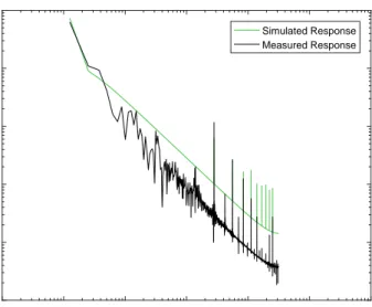
Using the gathered system output of X axis and prepared identification input, system model is calculated via the Matlab’s System Identification Toolbox. In Frequency domain, simulated system output fits to the measured system out-put % 86.34 . Also, it is also extremely crucial to show that system is not over fitted using a validation data set. Using the validation data set, simulated system output fit to the measured system output %84.2. So, it is safe to conclude that an acceptable fit is acquired while avoiding over fit. Transfer function is also validated in time domain in the following section.

10-2 10-1 100 101 102 103 104 Frequency (rad/s) 101 102 103 104 105 106 Amplitude Simulated Response Measured Response

Figure 2.8: Measured vs Simulated Response in Frequency Domain: X axis

10-2 ₁₀-1 ₁₀0 ₁₀1 ₁₀2 ₁₀3 ₁₀4 Frequency (rad/s) 101 102 103 104 105 106 Amplitude Simulated Response Measured Response

Figure 2.9: Measured vs Simulated Verification Response in Frequency Domain: X axis

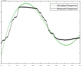
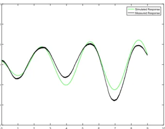
Time Domain Validation 0 5 10 15 20 25 30 35 40 45 50 Time -2 -1 0 1 2 3 4 Position (micrometers) ×104 Simulated Response Measured Response

Figure 2.10: Measured vs Simulated Response: X axis

As is show in the figure 2.10, simulated system output and measured system output are fairly close. Moreover the fit is calculated as %71.92 which can be considered to be good enough while avoiding the possibility of over fit.

Furthermore, as shown on the figure simulated response also fit to the measured verification data fairly well. The fit is calculated as %68.23.

Identified transfer function is;

Gxx =

5.693 × 104_{s + 1389}

s2_{+ 0.2268s + 0.002058} (2.3)

As shown in the table 2.1 all zeros and poles of the identified transfer function

Poles Zeros

-0.2173 -0.0244

-0.0095

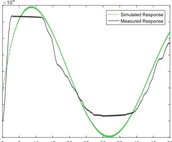
0 5 10 15 20 25 30 35 40 45 50 Time -0.5 0 0.5 1 1.5 2 2.5 3 3.5 Position (micrometers) ×104 Simulated Response Measured Response

Figure 2.11: Measured vs Simulated Verification Response: X axis

are in the left domain, therefore the identified transfer function is stable and minimum phase.

2.2.2.2 Y axis

Using the gathered system output of Y axis and prepared identification input, system model is calculated via the Matlab’s System Identification Toolbox. In Frequency domain, simulated system output fits to the measured system out-put % 80.13 . Also, it is also extremely crucial to show that system is not over fitted using a validation data set. Using the validation data set, simulated system output fit to the measured system output %68.21 So, it is safe to conclude that an acceptable fit is acquired while avoiding over fit. Transfer function is also validated in time domain in the following section.

10-2 10-1 100 101 102 103 104 Frequency (rad/s) 100 101 102 103 104 105 106 Amplitude Simulated Response Measured Response

10-2 ₁₀-1 ₁₀0 ₁₀1 ₁₀2 ₁₀3 ₁₀4 Frequency (rad/s) 100 101 102 103 104 105 106 Amplitude Simulated Response Measured Response

Figure 2.13: Measured vs Simulated Verification Response in Frequency Domain: Y axis

Time Domain Validation

As is show in the figure 2.14, simulated system output and measured system output are fairly close. Moreover the fit is calculated as %77.69 which can be considered to be good enough while avoiding the possibility of over fit.

Also as shown on the figure, simulated response also fit to the measured verifica-tion data fairly well. The fit is calculated as %64.78. Identified transfer funcverifica-tion is;

Gyy =

5.48 × 105_{s + 1.367 × 10}4

0 1 2 3 4 5 6 7 8 9 10 Time -1.5 -1 -0.5 0 0.5 1 Position (micrometers) ×104 Simulated Response Measured Response

Figure 2.14: Measured vs Simulated Response in Time Domain: Y axis

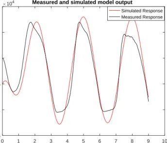
0 1 2 3 4 5 6 7 8 9 10 Time -1.5 -1 -0.5 0 0.5 1 Position(micrometers)

×104 Measured and simulated model output

Simulated Response Measured Response

Figure 2.15: Measured vs Simulated Verification Response in Time Domain: Y axis

As shown in the table 2.2, all zeros and poles of the identified transfer function are in the left domain, therefor the identified transfer function is stable and minimum phase.

Poles Zeros

-0.8181 ± 2.7415i -0.0249

2.2.2.3 Z axis

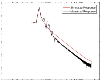
Using the gathered system output of Y axis and prepared identification input, system model is calculated via the Matlab’s System Identification Toolbox. In Frequency domain, simulated system output fits to the measured system out-put % 67.44 . Also, it is also extremely crucial to show that system is not over fitted using a validation data set. Using the validation data set, simulated system output fit to the measured system output %72.03 So, it is safe to conclude that an acceptable fit is acquired while avoiding over fit. Transfer function is also validated in time domain in the following section.

10-2 10-1 100 101 102 103 104 Frequency (rad/s) 10-2 100 102 104 106 Amplitude Simulated Response Measured Response

10-2 10-1 100 101 102 103 104 Frequency (rad/s) 10-2 100 102 104 106 Amplitude Simulated Response Measured Response

Figure 2.17: Measured vs Simulated Verification Response in Frequency Domain: Z axis

Time Domain Validation

As is show in the figure 2.18 , simulated system output and measured system output are fairly close. Moreover the fit is calculated as %67.89 which can be considered to be good enough while avoiding the possibility of over fit.

Furthermore, as shown on the figure simulated response also fit to the measured verification data fairly well. The fit is calculated as %72.04

Identified transfer function is;

Gzz =

3.556 × 105_{s + 5.468 × 10}6

s3_{+ 607.5s}2_{+ 344s + 2643} (2.5)

Using these identified transfer functions, robust controller is synthesized in the following chapter.

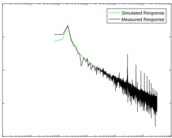
0 1 2 3 4 5 6 7 8 9 10 Time (s) -3000 -2000 -1000 0 1000 2000 3000 Position (Micrometers) Simulated Response Measured Response

Figure 2.18: Measured vs Simulated Response in Time Domain: Z axis

Poles Zeros

-0.2798 ± 2.0679i -15.37

-606.91

Table 2.3: Poles and Zeros: Gzz

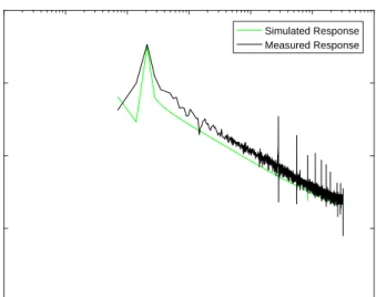
0 1 2 3 4 5 6 7 8 9 10 Time (s) -3000 -2000 -1000 0 1000 2000 3000 Position (Micrometers) Simulated Response Measured Response

Figure 2.19: Measured vs Simulated Verification Response in Time Domain: Z axis

Chapter 3

Robust Controller Synthesis

3.1

H

Problem

Figure 3.1: General Control Problem Structure for H∞.

The general H∞ control structure is give above; where w, z, u and y are external

inputs, outputs, Control signals and measured variables respectively.

Defining Fl(G, K) = Tzwas the transfer matrix from external inputs (w) to output

The H∞ optimization problem is to find a stabilizing controller K which will

minimize the infinity norm of the Tzw which can be expressed mathematically as

equation 3.2 ; min K∈H∞ kTzwk∞= min K∈H∞ { sup Re(s)>0 ¯ σ[Tzw(s)]} (3.2)

3.2

Loop Shaping

Generally desired Tzw has distinct behaviors on distinct frequency bands. Two

most commonly used performance measures are sensitivity (S) and complemen-tary sensitivity (T ) functions. (Whereas S + T = I) So if weight functions such

as Ws and Wt are implemented then the problem becomes;

kTzwk∞ = w w w w w w WsS WtT w w w w w w < γ (3.3)

Ws and Wt are constructed to achieve desired goals and desired frequency bands.

For instance, generally S is minimized at low frequencies to achieve better track-ing and disturbance attenuation where T is minimized at high frequencies to achieve robust stability in the presence of sensor noise, variations in the system parameters and un-modeled high-order dynamics.

3.3

H

Controller Synthesis For Micro-Machining

System

As identified on the previous chapter, the transfer function of x,y and z axis’s are as follows. Gxx = 5.693104_{s + 1389} s2_{+ 0.2268s + 0.002058} (3.4) Gyy = 5.48105_{s + 1.36710}4 s3 _{+ 1.644s}2 _{+ 8.198s + 0.06571} (3.5) Gzz = 3.5561005s + 5.468e06 s3_{+ 607.5s}2_{+ 344s + 2643} (3.6)

3.3.1

Weighting Functions

In order to synthesize H∞controller for the system, first of all the weight functions

need to be designed. Even tough there are some guidelines for the weight function design, fine tuning using the simulations is necessary. The weight function form used to synthesize the controller is proposed by Allgower. [11]. Such as;

Ws = W1 = s M + ω0 s + ω0A (3.7) W2 = 1 max co (3.8) Wt= W3 = ω0 M + s As + ω0 (3.9)

where; ω0 is the desired bandwidth; M is the sensitivity peak; A is the steady

state error;

These weight functions tuned manually using simulations. Moreover during the fine tuning of the weight functions, guidelines specified by Bibel [12] and Beaven [13] are followed. Final weighting functions for the axis’s are given below;

3.3.1.1 X Axis

For X axis weight functions; the parameters chosen as; A = 0.001, M = 2 and

ω0 = 160 which gives weight function as follows;

Ws = W1 = 0.5 s + 320 s + 0.16 (3.10) W2 = 1 10 (3.11) Wt = W3 = 1000 s + 80 s + 1.6 × 105 (3.12)

-20 0 20 40 60 Magnitude (dB) 10-2 10-1 100 101 102 103 104 -90 -45 0 Phase (deg) Frequency (rad/s)

Figure 3.2: Weight Function: Ws of X Axis

-20 0 20 40 60 Magnitude (dB) 100 102 104 106 0 45 90 Phase (deg) Frequency (rad/s)

3.3.1.2 Y Axis

For Y axis weight functions; the parameters chosen as; A = 0.001, M = 2,

ωs0 = 150 and ωt0= 180 which gives weight function as follows;

Ws = W1 = 0.5 s + 300 s + 0.15 (3.13) W2 = 1 10 (3.14) Wt = W3 = 1000 s + 90 s + 1.8 × 105 (3.15) -20 0 20 40 60 Magnitude (dB) 10-2 10-1 100 101 102 103 104 -90 -45 0 Phase (deg) Frequency (rad/s)

-20 0 20 40 60 Magnitude (dB) 100 102 104 106 0 45 90 Phase (deg) Frequency (rad/s)

Figure 3.5: Weight Function: Wt of Y Axis

3.3.1.3 Z Axis

For Z axis weight functions; the parameters chosen as; A = 0.01, M = 2 and

ω0 = 120 which gives weight function as follows;

Ws = W1 = 0.5 s + 240 s + 1.2 (3.16) W2 = 1 10 (3.17) Wt= W3 = 100 s + 60 s + 1.2 × 104 (3.18)

-10 0 10 20 30 40 Magnitude (dB) 10-2 10-1 100 101 102 103 104 -90 -45 0 Phase (deg) Frequency (rad/s)

Figure 3.6: Weight Function: Ws of Z Axis

-10 0 10 20 30 40 Magnitude (dB) 100 101 102 103 104 105 106 0 45 90 Phase (deg) Frequency (rad/s)

3.3.2

Synthesized Robust Controllers

Using the weight functions presented in the previous section, robust H∞

con-trollers are designed using Matlabs hinfsyn command for the each individual axis. These synthesized controllers are, then implemented in the simulation and actual system to measure performance and improvements compared to the CC PID controller.

3.3.2.1 X Axis

The synthesized H∞ controller for the X axis is:

Gxx = 5.2563105×

(s + 1.6104_{)(s + 0.2173)(s + 0.009474)}

(s + 5.693107_{)(s + 5.26610}4_{)(s + 1.6)(s + 0.0244)} (3.19)

3.3.2.2 Y Axis

The synthesized H∞ controller for the Y axis is:

Gyy = 2881.1

(s + 1.8 × 105)(s + 0.008028)(s2+ 1.636s + 8.185)

(s + 1.773 × 105_{)(s + 3.09 × 10}4_{)(s + 420.1)(s + 0.15)(s + 0.02494)}

(3.20)

3.3.2.3 Z Axis

The synthesized H∞ controller for the Z axis is:

Gyy = 2881.1

3.8912 × 105_{(s + 1.2 × 10}4_{)(s + 606.9)(s}2_{+ 0.5597s + 4.354)}

(s + 3.892 × 104_{)(s + 15.38)(s + 1.2)(s}2_{+ 2.957 × 10}4_{s + 3.585 × 10}8₎

3.4

Simulations

3.4.1

Simulation Design

In order to carry out the simulations, a system model with X, Y and Z axis’s is created in Simulink software. In this model, transfer functions identified in

chapter (Gxx, Gyy and Gzz) is used. Then either CC PID or synthesized robust

controller is added to the system model. Furthermore the input signals of X, Y and Z axis’s are created using S curves with a Matlab script offline. That input signal is fed into the simulation setup and output data is logged.

Cross Coupled PID Controller

The PID controller used in the simulations and experiments are CC PID Con-troller. The Control diagram of the controller is given in the figure 3.9.

Figure 3.9: CC PID Controller

Cross-Coupled PID used over conventional PID to decrease the contouring error. The Cross-Coupled controller algorithm for the positioning system designed by Erva Ulu.[14] But in order to use that controller for the micro-milling system, the CC PID controller parameters is re-tuned manually.

Contour Error

Contour error can be calculated using geometrical relations of error vectors. This vectorial approach can be explained using the geometrical relations in the given

figure. In the given figure, ~e is the tracking error vector, ~ˆε is estimated contour

error vector, ~ε is contour error vector, ~t is normalized tangential vector, ~n is

Then the contouring error ~ε can defined as the vector from the actual position to the nearest point on the line which passes through the reference position tangen-tially with direction ~t . [18]

Figure 3.10: Geometric Relations Of Contour Error

3.4.2

Simulation Results- Without Disturbance

For this simulation, the simulation setup run shown in the previous section run without any disturbance input. The desired shape is an inclined circle with a diameter of 5 mm and an incline angle of 45 deg.

3.4.2.1 CC PID Controller

In this simulation an inclined circle is tracked by system using PID controllers. In total, there are 4 PID controllers; X, Y, Z and CC controller. The parameters of PID controller are given at the table 3.1.

-5000 -4000 2000 -3000 0 1000

Z Position (in micrometers)

-2000

-1000

Y Position (in micrometers)

-1000

0 _-2000

X Position (in micrometers)

0

-1000 -3000

-4000 -2000

-5000

Figure 3.11: Desired Output

PID Paramters P I D N

X 1 0.01 0.0005 100

Y 1.5 0.01 0.0005 100

Z 1 0.01 0.0005 100

CC 0.4 0.005 0.0005 100

-5000 -4000 -3000 -2000 -1000 0

X Position (in micrometers)

-3000 -2000 -1000 0 1000 2000

Y Position (in micrometers)

Simulation Output Desired System Response

Figure 3.12: Desired Output vs Simulation Output with PID Controller: X vs Y

-2000 -1000 0 1000 2000 3000

Y Position (in micrometers)

-5000 -4000 -3000 -2000 -1000 0

Z Position (in micrometers)

Simulation Output Desired System Response

0 2 4 6 8 10 12 14 16 18 20 Time (seconds) -200 -150 -100 -50 0 50 100 150

Error in X axis (micrometers)

Figure 3.14: Error vs Time with PID Controller: X axis

0 2 4 6 8 10 12 14 16 18 20 Time (seconds) -100 -80 -60 -40 -20 0 20 40 60 80 100

Error in Y axis (micrometers)

0 2 4 6 8 10 12 14 16 18 20 Time (seconds) -200 -150 -100 -50 0 50 100 150

Error in Z axis (micrometers)

Rms Errors (micrometers)

Ex 53.29

Ey 34.61

Ez 53.28

Ec 26.24

Table 3.2: Rms Errors: PID Controller

The desired and simulated outputs of xy and yz planes are given. Moreover, the error signals of the each axis is also given. In this not-disturbed simulation PID

controller achieved acceptable results. The rms values of the Ex, Ey, Ez and Ec

signals are given in the table.

3.4.2.2 Robust Controller

In this simulation the same inclined circle is tracked by system using Robust con-trollers. There are 3 robust controllers; X, Y and Z concon-trollers. The Controllers are as follows; Gxx = 5.2563105 (s + 1.6104_{)(s + 0.2173)(s + 0.009474)} (s + 5.693107_{)(s + 5.26610}4_{)(s + 1.6)(s + 0.0244)} (3.22) Gyy = 2881.1 (s + 1.8 × 105)(s + 0.008028)(s2+ 1.636s + 8.185) (s + 1.773 × 105_{)(s + 3.09 × 10}4_{)(s + 420.1)(s + 0.15)(s + 0.02494)} (3.23) Gyy = 2881.1 (3.8912 × 105)(s + 1.2 × 104)(s + 606.9)(s2+ 0.5597s + 4.354) (s + 3.892 × 104_{)(s + 15.38)(s + 1.2)(s}2_{+ 2.957 × 10}4_{s + 3.585 × 10}8₎ (3.24)

-5000 -4500 -4000 -3500 -3000 -2500 -2000 -1500 -1000 -500 0

X Position (in micrometers)

-2500 -2000 -1500 -1000 -500 0 500 1000 1500 2000 2500

Y Position (in micrometers)

Simulation Output Desired System Response

Figure 3.17: Desired Output vs Simulation Output with Robust Controller: X vs Y

-2500 -2000 -1500 -1000 -500 0 500 1000 1500 2000 2500

Y Position (in micrometers)

-5000 -4500 -4000 -3500 -3000 -2500 -2000 -1500 -1000 -500 0

Z Position (in micrometers)

Simulation Output Desired System Response

Figure 3.18: Desired Output vs Simulation Output with Robust Controller: Y vs Z

0 5 10 15 Time (seconds) -60 -50 -40 -30 -20 -10 0 10

Error in X axis (micrometers)

Figure 3.19: Error vs Time with Robust Controller: X axis

0 5 10 15 Time (seconds) -40 -30 -20 -10 0 10 20 30

0 5 10 15 Time (seconds) -60 -50 -40 -30 -20 -10 0 10

Error in Z axis (micrometers)

Rms Errors - Robust Controller (micrometers) Improvement Over PID Controller

Ex 25.32 %52.49

Ey 6.60 %80.93

Ez 28.88 %45.8

Ec 32.09 -%18.23

Table 3.3: Rms Errors: Robust Controller

When the error values of Robust Controller compared to PID controller, it could be concluded that even without a disturbance signal robust controller improve tracking. But also, it must be noted that the rms of contour error is higher when using the robust controller(26.24 to 32.09 micrometers) This is caused by the lack of a separate contour controller. It is safe to assume that, contouring error could be effectively decreased with the addition of a robust contour controller.

3.4.3

Simulation Results - With Disturbance

For this simulation, the simulation setup run shown in the previous section run with sinusoidal disturbance input in each axis. The amplitude of the disturbance is 100 micrometers and the frequency is 75 rad/s. This position disturbance is injected to system after the plant. The desired shape is again an inclined circle with a diameter of 5 mm and an incline angle of 45 deg.

3.4.3.1 CC PID Controller

In this simulation an inclined circle is tracked by system using PID controllers. There are 4 PID controllers. X, Y, Z and CC controller. The error signals of the X, Y and Z axis’s are given below.

0 2 4 6 8 10 12 14 Time (seconds) -400 -300 -200 -100 0 100 200 300 400

Error in X axis (micrometers)

Figure 3.22: Error vs Time with PID Controller: X axis

0 2 4 6 8 10 12 14 Time (seconds) -300 -200 -100 0 100 200 300

Error in Y axis (micrometers)

0 2 4 6 8 10 12 14 Time (seconds) -400 -300 -200 -100 0 100 200 300 400

Error in Z axis (micrometers)

Error values increased substantially with the addition of the disturbance input. Moreover the error of X, Y and Z axis’s often crosses the disturbance signals amplitude of 100 micrometers which shows that the disturbance rejection property is not acceptable with the CC PID controller. The rms values of the errors are given in the table 3.4. Also, it must be noted that the rms value of X and Y error signals are bigger than the disturbance inputs maximum amplitude, which clearly show that the disturbance rejection of th CC PID controller is sub par.

Rms Errors - PID Controller

Ex 146.69

Ey 138.82

Ez 146.7

Ec 108.32

Table 3.4: Rms Errors with Disturbance Input: PID Controller

3.4.3.2 Robust Controller

In this simulation an inclined circle is tracked by system using Robust controllers. There are 3 PID controllers. X, Y and Z controllers. The Controllers are as follows; Gxx = 5.2563105 (s + 1.6104_{)(s + 0.2173)(s + 0.009474)} (s + 5.693107_{)(s + 5.26610}4_{)(s + 1.6)(s + 0.0244)} (3.25) Gyy = 2881.1 (s + 1.8 × 105_{)(s + 0.008028)(s}2_{+ 1.636s + 8.185)} (s + 1.773 × 105_{)(s + 3.09 × 10}4_{)(s + 420.1)(s + 0.15)(s + 0.02494)} (3.26) Gyy = 2881.1 (3.8912 × 105)(s + 1.2 × 104)(s + 606.9)(s2+ 0.5597s + 4.354) (s + 3.892 × 104_{)(s + 15.38)(s + 1.2)(s}2_{+ 2.957 × 10}4_{s + 3.585 × 10}8₎ (3.27) The error signals of the X, Y and Z axis’s are given below.

0 5 10 15 Time (seconds) -100 -50 0 50

Error in X axis (micrometers)

Figure 3.25: Error vs Time with Robust Controller: X axis

0 5 10 15 Time (seconds) -150 -100 -50 0 50 100 150

0 5 10 15 Time (seconds) -120 -100 -80 -60 -40 -20 0 20 40 60 80

Error in Z axis (micrometers)

Figure 3.27: Error vs Time with Robust Controller: Z axis

Rms Errors - Robust Controller (micrometers) Improvement Over PID Controller

Ex 42.12 %72.29

Ey 74.76 %46.15

Ez 52.13 %64.46

Ec 69.02 %36.28

The significant decrease of the rms errors show that robust controller’s distur-bance rejection property is far greater than CC PID controller. Also, none of the axis’s rms error value is greater than the amplitude of disturbance signal. More-over, when the improvements are examined, the least improvement is %36.28. So it is safe to say that, according to the simulations robust controller is far more suited to a machining system where many unavoidable disturbance signals present.

Chapter 4

Micro-machining Experiments

Micro-machining system consists of a 3-axis positioning system and spindle. 3 axis-positioning system is controlled using CC PID controller or synthesized ro-bust controllers. Spindle has its own controller, which can be set between 1 and 60k rpm’s. In the connection of 3-axis positioning system and the lab PC NI card’s used. Implementation of the controllers done in the Labview program. A photo of the system is given in Figure 4.1

In order to evaluate the performance of the micro-machining system, several experiments conducted using both the robust and PID controller. Results of these tests, with PID and Robust controller and the comparison of the two is given in the following sections respectively.

Figure 4.1: Micro-Machining System

4.1

PID with CCC Controller

Firstly, micro-machining experiments carried out with PID-CCC controller. For this experiments several input signals (cutting paths) are generated. These input signals are generated using S-Curves in order to limit the jerk to have a smooth path for the positioning system. The usage of S-curve also minimizes the effects of cross-coupling.

4.1.1

Circular Cutting Test

For this test, a circular cut is performed in order to test both the tracking per-formance while machining and the disturbance rejection to the cutting forces of the system. The diameter of the circle is designed to be 1 cm. The Input signals and the optical microscope image are given in the following figures. In this test a cutting speed of 35 krpm/min and a feed rate of 4mm/min is used. A depth of 150 micrometers is designed for circular cutting test, but because of the manual homing of the system, final depth of the manufacturing is error prone.

-5000 -4500 -4000 -3500 -3000 -2500 -2000 -1500 -1000 -500 0

Y axis position (micrometers)

-2500 -2000 -1500 -1000 -500 0 500 1000 1500 2000 2500

Z axis position (micrometers)

Figure 4.2: Input Signal: Z vs Y axis

According to the Optical microscope image of the circular cut, the diameter of the cut is 5021 micrometers. So the error in the diameter of the cut is %0.4. But it must be noted that, because of the cutting forces an oscillation is observed which degrades the surface quality. Also there is a major artifact produced because of that oscillation. (This artifact shown in the Figure 4.6 with red circle) Measured depth is 145 micrometers.

0 50 100 150 200 250 300 350 400 Time (s) -5000 -4500 -4000 -3500 -3000 -2500 -2000 -1500 -1000 -500 0

Y axis Position (Micrometers)

Figure 4.3: Input Signal: Y vs Time

0 50 100 150 200 250 300 350 400 Time (s) -2500 -2000 -1500 -1000 -500 0 500 1000 1500 2000 2500

0 0.2 0.4 0.6 0.8 1 1.2 1.4 1.6 1.8 2 Time (s) 0 50 100 150

X axis Position (Micrometers)

Figure 4.5: Input Signal: X vs Time

4.1.2

Square Cutting Test

The final cutting test is the square cutting test. For this test, a square cut is performed in order to test both the tracking performance while machining and the disturbance rejection to the cutting forces of the system. It must be noted that since square shape has sharp turns at corners, the disturbance caused by the cross axis effects has a larger effect compared to the circular cutting test. The length of a side of the square to be cut is 5mm’s. The Input signals and the optical microscope image are given in the following figures. A depth of 200 micrometers is designed for square cutting test, but because of the manual homing of the system, final depth of the manufacturing is error prone.

0 1000 2000 3000 4000 5000

Y axis position (micrometers)

-5000 -4000 -3000 -2000 -1000 0

Z axis Position (Micrometers)

Figure 4.7: Input Signal: Z vs Y axis

According to the Optical microscope image of the square cut, the side lengths of the square are 5047 and 5058 micrometers. So the error in the side length of the cut is %1.16. But it must be noted that, similar to the circular cutting test there are oscillations during machining. Because of the oscillations, there are

0 50 100 150 200 250 300 Time (s) 0 1000 2000 3000 4000 5000 6000

Y axis Position (Micrometers)

Figure 4.8: Input Signal: Y vs Time

quality can be easily seen in the optical microscopy image. Measured depth is 190 micrometers.

0 50 100 150 200 250 300 Time (s) -6000 -5000 -4000 -3000 -2000 -1000 0

Z axis Position (Micrometers)

Figure 4.9: Input Signal: Z vs Time

0 50 100 150 200 250 Time (s) 1000 2000 3000 4000 5000 6000 7000 8000

6 8 10 12 14 16 Time (s) 7100 7150 7200 7250 7300 7350

X axis Position (Micrometers)

Figure 4.11: Input Signal: X vs Time

4.2

Robust Controller

4.2.1

Circular Cutting Test

Circular cutting experiment is carried out with robust controller. The input signals for this circular cutting test is same with the PID test input signals. The optical microscopy image is given below.

Figure 4.13: Optical Microscope Image Of the Circular Cut

According to the optical microscopy image the error in the radius is %2.38. In contrast to CC PID controller the error in radius is higher. On the other hand, the surface quality is significantly better. Moreover, there aren’t any artifacts which do exist in CC PID controller. Also, it must be noted that oscillations, do not occur in robust controller opposed to CC PID controller. Measured depth is 123 micrometers.

4.2.2

Square Cutting Test

Square cutting experiments carried out with robust controller. The input signals for this square cutting test is same with the PID test input signals. The opti-cal microscopy image of the square cut is given below. Measured depth is 182 micrometers.

Figure 4.14: Optical Microscope Image Of the Square Cut

According to the optical microscopy image the error in the side length is %0.07 (The error in the side length was %1.16 with PID controller). In contrast to CC PID controller the error in side length is significantly smaller. Even with a smooth S-curve the square cutting test has sharp turns at the edges. These sharp turns, increase the effect of cross-coupling which could be the reason of this dramatic decrease in side length error in robust controller. Furthermore, the surface is better compared to the CC PID Controller. Also, it must be noted that the oscillations, do not occur in robust controller opposed to CC PID controller.

Chapter 5

Conclusion

As a result of the miniaturization, micro-manufacturing has became one of the most popular topics. Even tough there are new promising micro manufacturing techniques, micro machining will not be obsolete any time soon. This theses has aimed to develop a robust controller algorithm for a three-axis micro machining system.

In chapter II, first of all, the system is identified and modeled in order to synthe-size the controller. It must be noted that these identified transfer function should be representing the system without over-fit. Moreover these identified transfer functions are verified using similar but different identification inputs.

In chapter III, H∞ robust controllers for X,Y and Z axis’s are synthesized using

both the identified transfer functions and designed weighting functions. Simula-tion results showed significant improvements on both with disturbance or without the disturbance case. Especially, in the disturbed case, there are improvements up to %70, on the tracking performance.

At last but not least, in chapter V the synthesized controller implemented on the micro machining system to conduct cutting experiments. According to ex-periment results, robust controller showed similar dimensional performance with

improved stability. But it must be noted that even tough the dimensional per-formance is similar in circular manufacturing test there is a significant decrease in the error in square cutting test(%0.07 with Robust Controller %1.16 with PID controller). The most prominent improvement is the lack of oscillations while manufacturing. Furthermore, there are significantly less artifacts on the manufactured parts with the robust controller.

For further research, design and implantation of a CC robust controller could be examined. According to results of this thesis, it is safe to assume that, a CC robust controller will be have better tracking capabilities compared to PID or (non-CC) robust controller while maintaining stability. Moreover, identified transfer functions could be improved by using filters to cut high frequency noise in the acquired data sets. At last but not least, for all tests, the micro-manufacturing system assumed to be rigid and having very low manufacturing tolerances. The actual deflections in the system while manufacturing may increasing the error. So tests about the systems deflections and rigidity while manufacturing, could be very used to reduce the total error.

Bibliography

[1] R. Feynman, “There’s plenty of room at the bottom: An invitation to enter a new physics,” Engineering and Science, Caltech, February 1960.

[2] T.-R. Hsu, “Miniaturization: A paradigm shift in advanced manufacturing and education,” Microsystems Design and Packaging Laboratory Depart-ment of Mechanical and Aerospace Engineering San Jose, California, USA. [3] K. A. M. Adem, R. Fales, and A. S. El-Gizawy, “Identification of cutting force

coefficients for the linear and nonlinear force models in end milling process using average forces and optimization technique methods,” The International Journal of Advanced Manufacturing Technology, vol. 79, no. 9, pp. 1671– 1687, 2015.

[4] L. S. Stephens and C. R. Knospe, “µ-synthesis based, robust concontrol design for amb machinig spindles,” in Fifth International Symposium on Magnetic Bearings, August 1996.

[5] H. S. Lee and M. Tomizuka, “Robust motion controller design for high-accuracy positioning systems,” IEEE Transactions on Industrial Electronics, vol. 43, pp. 48–55, Feb 1996.

[6] A. R. Kashani, J. W. Sutherld, K. Moon, and J. Michler, “A robust control scheme for improved machinig surface texture,” NAMRI/SME, vol. XXI, pp. 429–434, 1993.

track-Journal of Dynamic Systems, Measurement, and Control, vol. 116, pp. 24– 32, March 1994.

[8] B. Yao, M. Al-Majed, and M. Tomizuka, “High-performance robust motion control of machine tools: An adaptive robust control approach and com-parative experiments,” IEEE/ASME Transactions on Mechatronics,, vol. 2, pp. 63–76, June 1997.

[9] H. Moradi, G. Vossoughi, and M. d R. Movahhedy, “Robust control of regen-erative chatter in peripheral milling process,” Centre of Excellence in Design, Robotics and Automation (CEDRA), Department of Mechanical Engineer-ing, Sharif University of Technology, Tehran, Iran.

[10] N. G. Ulu, E. Ulu, and M. Cakmakci, “Adaptive correction and look-up table based interpolation of quadrature encoder signals,” in ASME 2012 5th Annual Dynamic Systems and Control Conference joint with the JSME 2012 11th Motion and Vibration Conference, vol. 2, pp. 543–552, American Society of Mechanical Engineers, 2012.

[11] F. Allgower, “H-infinity control,” Universitat Stuttgart. Institut f¨ur

Sys-temtheorie und Regelungstechnik.

[12] J. E. Bibel and D. S. Malyevic, “Guidelines for the selection of weighting functions for h-infinity control,” January 1992.

[13] R. Beaven, M. Wright, and D. Seaward, “Weighting function selection in the

h∞ design process,” Control Eng. Practice, vol. 4, no. 5, pp. 625–633, 1996.

[14] N. G. Ulu, E. Ulu, and M. Cakmakci, “Learning based cross-coupled control for multi-axis high precision positioning systems,” in ASME 2012 5th Annual Dynamic Systems and Control Conference joint with the JSME 2012 11th Motion and Vibration Conference, vol. 2, pp. 535–541, American Society of Mechanical Engineers, 2012.

[15] MATLAB, version 9.10.0 (R2015b). Natick, Massachusetts: The

[16] T. M. Inc., Control System Toolbox: User’s Guide. Natick, Massachusetts, 10.0 ed., 2016.

[17] L. Ljung, System Identification Toolbox: User’s Manual. The MathWorks Inc., Natick, Massachusetts, 10.0 ed., 2016.

[18] S.-S. Yeh and P.-L. Hsu, “Estimation of the contouring error vector for the cross-coupled control design,” IEEE/ASME transactions on mechatronics, vol. 7, no. 1, pp. 44–51, 2002.

Appendix A

Block Diagram

Block Diagram of the System given in the following pages. Because of the size, block diagram cannot be given in a single page, block diagram can be formed by placing the following pages together.