Modeling for green growth: environmental policy in a dualistic peripheral economy

Macroeconomics of Climate Change in a Dualistic Economy Copyright © 2018 Elsevier Inc.

http://dx.doi.org/10.1016/B978-0-12-813519-8.00004-2 All rights reserved. ₉₃

Modeling for Green Growth:

Environmental Policy in a

Dualistic Peripheral Economy

The main methodological apparatus of this study is now introduced. The overall characteristics of this quantitative and analytical approach and ini-tially introduced, and its salient features are discussed in contrast to alter-native modeling techniques that have been reported in the literature. This modeling framework rests on the theoretical basis of general equilibrium with various economic activities across many markets, as interplayed by diverse actors, households, producers, governmental bodies, and the foreign economy.

Thus the focus of this chapter is on the nature and consequences of the dynamic interplay of general equilibrium interactions. It is set within the context of structural characteristics of a developing economy (i.e., Turkey) to reveal regional stratification and duality. The analytical approach is based on the methodology of applied general equilibrium distinguished as the folklore of computable general equilibrium (CGE). The methodological rationale is based on the urgent need to improve understanding of the com-plex trade-offs between attaining sustainable development, mitigating the threat of climate change, and enhancing social welfare. The need to identify an analytical resolution for ranking alternative policy instruments and inter-actions from the point of view of social welfare and economic well-being will also be addressed.

The CGE modeling methodology is the most conducive analytical ap-paratus for capturing these diverse objectives and policy trade-offs within the discipline of general equilibrium theory. Embedded in the theoretical realm of the Walrasian equilibrium, the CGE framework provides a coher-ent system of data managemcoher-ent and scenario analyses to simultaneously address issues of sustainability and mitigation.

The concept of developmental sustainability is a fairly recent phenom-enon that came into development economics through the 1987 report of the World Commission on Environment and Development led by the Brundtland Commission. The Brundtland report succinctly summarized the concept as

“… development which meets the needs of the present without compro-mising the ability of future generations to meet their own needs.” Sustain-ability has since become one of the most influential phrases of the environ-mental policy agenda.

Thus what is needed is a coherent analysis of the systemic relations sur-rounding the energy–economy–environment (3E) nexus. Thus the CGE framework is utilized as a social laboratory tool for addressing policy ques-tions over the 3E realm.

4.1 THE CGE FOLKLORE

The CGE methodology is an applied approach to the Walrasian economic system. It is Walrasian in the sense that it brings behavioral assumptions, pro-duction technologies, and market institutions together within the discipline of general equilibrium. Along with equilibrium production processes, it also brings factors of production (i.e., capital, labor, and energy aggregate input) within a dynamically adjusting technological pathway.

Commensurate with production activities, incomes are generated through wages, profits, and other factor payments. Income remunerations are channeled to the households whose role in the system is to dispose of the generated factor income through (private) consumption expenditure on commodities or (private) savings. Saving funds are, in turn, disposed of as investment expenditures on fixed capital to accentuate the potential output in the next production cycle.

Following the identification of national income accounting, any gap in the domestic savings–investment balance is met by foreign savings; that is, the balance on the current account of the balance of payments. Adjustments on a flexible (real) exchange rate (conversion factor of the price indexes of domestically produced versus foreign goods), or quantity adjustments on foreign exchange flows, are possible modes to bring forth the warranted equilibrium. Governments are institutionalized in every aspect of economic activity considered thus far. Through the administration of taxation or sub-sidization, governments can act as economic agents to fulfil public expen-diture or saving accounts, and function as administrative units to design alternative policy scenarios and implement instruments of abatement. The CGE framework has the capability to provide an economic evaluation of “what if?” policy interventions under various abatement scenarios.

Thus given their structural flexibility and theoretical consistency, CGE models have become standard tools for the quantitative analysis of policy

inference by international agencies (i.e., the Organisation for Economic Co-operation and Development (OECD) and the World Bank) and nu-merous national bodies of developmental and environmental policy. Deeper surveys are provided by Bergman (1990), Bhattacharyya (1996), Böhringer and Löschel (2006), and Shoven and Whalley (1992).

Chapter 2 briefly discussed the basic dual-economy model and the models of structural transformation, building on the earlier works of Higgins (1956), Jorgenson (1961, 1966, 1967), Lewis (1954), and Ranis and Fei (1961). The CGE literature offers a sophisticated platform to study the basics of the dual-economy model, such as interdependencies among differ-ent sectors of the economy, productivity differences between modern and traditional sectors, patterns of unemployment and underemployment, la-bor market imperfections, and dynamics of (qualitatively) different types of growth-capital accumulation. With high levels of data disaggregation, CGE models also provide substantial gains in the move towards more realistic structures (de Melo, 1977; Sue Wing, 2004; Temple, 2005).

The reflection of the model on “modern sector dualism” puts consider-able focus on labor market (or market) imperfections, of which the effects project onto the labor markets. Imperfect or segmented labor markets have implications for sectoral production structures, sectoral productivity differ-entials, and aggregate outcomes (Temple, 2004). Multisectoral CGE models are therefore useful, and required, in the analysis of interactions between urban unemployment, informal sector size, and structural transformation and economic growth patterns.

Understanding structural change and its determinants clearly has direct policy implications. Applied multisectoral general equilibrium models that provide detailed accounts of the economic structure in developing econo-mies are often used to assess policy alternatives and have long-term impacts (i.e., climate change). These models offer a framework with multisectors, different production structures, detailed representations of the labor mar-kets, possible migration dynamics, and regional specialization. They are also capable of providing modern accounts of the interactions between long-term structural transformation and the distribution of welfare. Hence CGE models with basic “dualistic” structures are extensively utilized to study inequality and poverty.

Representation of the well-documented features of the labor market in developing countries (i.e., wage efficiency, a large informal sector, labor market segmentation, a heterogeneous and imperfectly mobile labor force, and wage flexibility in the informal sector) allows these models to study the

strong links between the structure of the labor markets, the transmission of policy shock, and inequality and poverty (Agénor, 2004). Many classical CGE models work with homogenous labor markets with a fixed supply of labor and flexible wages; however, the models that aim to analyze poverty and the poverty-reduction implications of policies (i.e., trade liberalization, structural adjustment, and social transference) engage in more detailed rep-resentation of the labor market, often accompanied with other dualistic attributes of developing economies.1

The representation of labor heterogeneity through the distinction be-tween formal and informal and urban and rural labor under various degrees of substitution forms the basic approach for developing “dual labor market” structures in applied general equilibrium modeling (Graafland et al., 2001; Hendy and Zaki, 2013). The basic idea of the Harris and Todaro (1970) framework, which stated that urban–formal and rural–informal labor mar-kets are not completely isolated from each other but are connected via (imperfect) labor mobility, has also been extensively utilized in CGE models studying poverty and inequality (Agénor et al., 2003; Alzua and Ruffo, 2011; Gilbert and Wahl, 2002; Yang and Huang, 1997).

The “dual–dual” structure adopted by Thorbecke (1993) not only uses the formal–informal labor characterization of these CGE models but fur-ther introduces coexisting modern and informal activities in both urban and rural areas, which is usually the case for typical middle-income devel-oping economies (Khan, 2004). Stifel and Thorbecke (2003) provide an example model of an archetype African economy to simulate the welfare effects of trade liberalization on poverty. The presence of dualism (modern and informal activities) within each sector makes it possible to analyze the distribution of both activities in rural and urban areas. Hence the single modeling framework captures a subsistence agriculture using traditional labor-intensive technologies, a large-scale capital-intensive agriculture pro-ducing mostly export goods, the urban–informal sector, and the urban– modern sector.2

2 _{Khan (2004) provides further discussion on the characteristics of applied general}

equilib-rium models for poverty policy analysis in the context of developing countries. He em-phasizes the importance of representing typical features including, market power, the role of intermediate and capital goods, the structure of financial systems, and the roles of labor markets and the informal sector.

1 _{Boeters and Savard (2012) provide a detailed review of alternatives for modeling labor}

Structuralist models, which focus on the role of demand to under-stand structural transformation, also provide examples of formal and infor-mal production structures in developing economies. Rada and von Armin (2014) and Morrone (2016) performed studies in India and Brazil, respec-tively. They highlighted the existence of formal and informal production activities with differentiated productivity levels, and emphasized the role of the informal sector in supplying the reservoir of labor for understand-ing the complexity of structural transformation dynamics in a middle-income developing economy. In a different framework, Roson and van der Mensbrugghe (2017) emphasized the importance of distinguishing be-tween the supply-side effects (which affect sectoral productivity and growth dynamics) and the demand-side effects (which capture the variations in the structure of final demand) for understanding structural transformation. Their results indicate that time-varying and income-dependent demand structures generate sizable variations in the industrial structure.

The relevance of regional modeling and regional CGE models in rep-resenting and analyzing the spatial distribution of “dualistic” structures, and the implications of such distributions on the structural transformation and geographical distribution of welfare in developing economies, should be noted. Regional and multiregional CGE models that emphasize the roles of the spatial distribution of production activities and (endogenous and im-perfect) interregional migration contribute to our understanding of dif-ferentiated development paths. Many regional CGE modeling reviews are available; however, Donaghy (2009), Giesecke and Madden (2012), Kraybill (1993), and Partridge and Rickman (2010) provide the basis for under-standing the effects of incorporating key regional features (i.e., regional labor markets and interregional migration) into structural transformation models.

The CGE approach is not the only method for quantitatively modeling the economics of climate change. A wide arsenal of quantitative methods exist to assess the complex set of interactions over the 3E nexus; however, a thorough survey is beyond the main focus of this study. Nevertheless, a brief synopsis of the alternative methods is instrumental in placing the CGE methodology in the right framework to emphasize its advantages and misconceptions.

The so-called macroeconometric models, mainly of Keynesian tradi-tion, have close affinity with the CGE model. These models rely on large datasets, often with long time series, and are amenable to statistical infer-ence and probabilistic hypothesis testing. However, they typically fail to

capture the cause–effect relationships between the economic machine and environmental pollution, and their analytical power at ranking the welfare implications of the policy instruments of abatement is rather limited. The CGE framework, with its theoretical basis laid out over the Walrasian gen-eral equilibrium foundation, can accommodate the structural cause–effect hypothesis over a wide range of behavioral motives and endogenous mar-ket signals. Furthermore, with their ability to make “what if?” assessments against a “business-as-usual” trajectory, their simulation exercises offer a vi-able metric for ranking the cause–effect impact of alternative policy regimes that combat climate change and mitigation.

Conversely, the nature of CGEs means that they can accommodate en-ergy sector activities through their production functions and characterize economic behavior in response to the cost minimization impulses of “ra-tional agents.” The CGE apparatus typically only addresses the workings of the energy system through the cost-value system of economic relations and, as such, may fail to provide sharp flows of the technical aspects of energy production and distribution.

An alternative take on the technical attributes of the energy system is ac-complished by the bottom-up approach of modeling. In contrast to the top-down CGE analysis, the bottom-up models attempt to capture the technical nature of the substitution possibilities and input requirements across the primary and final sources of energy production and distribution. They fo-cus exclusively on substitution and input requirements to produce a given energy throughput. As the cheapest method of energy substitutes, they at-tempt to offer the most efficient energy production technique that would indirectly serve as abatement projections.

However, a major deficiency of bottom-up methods is their lack of abil-ity to address energy–economy interactions. In particular, working typically within the constraints of fixed final demands, they do not accommodate feedback mechanisms from the economy to the energy system. In addition, they fail to offer much on the warranted implications of the policy instru-ments on the rate of growth, employment, and the path of capital invest-ments (the rebound effect).

However, it should be noted that this arguably diverse dichotomy does not necessarily pertain to a theoretical departure, but in the words of Böhringer and Löschel (2006, p. 50) it may “…simply relate to the level of aggregation and scope of ceteris paribus assumptions.” There have been various attempts to merge both approaches within a mega-framework, embedding the bottom-up energy module with the Walrasian

general equilibrium system of the simultaneous equations of a CGE (Böhringer, 1998; Manne, 1981).

Therefore there is not a single all-encompassing methodology. Start-ing with the general equilibrium theory for the socially-efficient instru-ments of abatement under informalization and duality within the context of the Turkish economy applied here, more steps ought to be investigated to advance our understanding of the complex dynamics between economy, society, and the environment.

4.1.1 Modeling the 3E Nexus via CGE Analytics

The version of the CGE model utilized in this study uses various methods to address the characteristic features of peripheral development and the dual objectives of development and environmental abatement. One distinguish-ing feature of the current model is that it deliberately recognizes regional differentiation in employment and production to accommodate the traps of poverty and technological backwardness. Turkey can be used as a viable example of a peripheral economy with a key mandate for sustaining energy sufficiency and generating growth and employment. However, the country is currently facing strong international pressure to bring its gaseous emis-sions under control. These constitute the main traits of the Turkey CGE model to be utilized in this study.

The model also takes account of the rigidities in the labor and capital markets by introducing explicit gaps against the equalization of the wage and profit rates across sectors. These “distortions” are set from the existing data on wage rates (and profit rates) across sectors, and are maintained as rigid divergences from equalization of the “average” wage rate. Migration is a further behavioral rule, which governs the movement of labor from poor regions (and its sectors) towards the affluent wage sectors of the high-income regions.

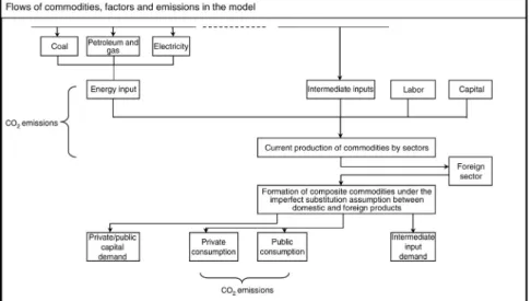
Environmental damage is mainly modeled in the form of gaseous pollu-tion. Greenhouse gas emissions (measured as CO₂ equivalents) are thought to be the end result of four sets of economic activities: (1) the combustion of fossil fuels to produce aggregate energy; (2) industrial processes used for the production of iron, steel, chemicals, and cement; (3) agricultural pro-cesses (mainly methane); and (4) household consumption and waste.

Submodeling of environmental pollution in the CGE apparatus recog-nizes these sources using technological parameters derived from the CO₂ eq. emissions inventory published by TurkStat. A bird’s-eye view of these relationships is portrayed in Fig. 4.1. Pollution is documented across the

energy-production activities and industrial and agricultural processes with-in the given production technologies. Waste is generated through consump-tion activities of private households.

The CGE methodology accommodates these activities by selecting the free parameters to fit the algebraic equation system to the base-year equilib-rium data, a procedure known as calibration. Calibration involves compilation of an annual dataset (in equilibrium) across its expenditures and revenues. Tabulated as a micro- and macrosystem of equilibrium relationships, this da-taset is referred to as the social accounting matrix (SAM) (Pyatt and Round (1979) provide a seminal introduction to the SAM system of accounts). The model’s algebraic specifications are then utilized to distill the parametric val-ues including the share parameters on production and consumption, key shift variables of numerous functional forms, and policy rates (i.e., taxes and sub-sidies). The “calibrated” model must be able to generate the original dataset disclosed in the SAM without any further statistical inference. This solution is known as the “base year.” Using a set of behavioral rules of capital accu-mulation and technical change alongside exogenous labor force (population) growth, dynamic CGE simulations set the stage for a base path.

The CGE exercises in this model will utilize the 2012 input–output (I/O) flow data published by TurkStat. Starting from the base year (2012), the algebraic system of general equilibrium will be accommodated by cali-brating the free parameters and shift variables as noted above.

The algebraic equations are introduced in a more formal format in the following section, which documents our data in the SAM system.

4.2 ALGEBRAIC STRUCTURE OF THE CGE MODEL

The model is composed of 17 production sectors spanning two regionalied bodies for the Turkish economy (high versus low income), a representative private household to carry out savings-consumption decisions, a govern-ment to implegovern-ment public policies towards environgovern-mental abategovern-ment, and a “rest of the world” account to resolve the balance of payment transac-tions. Antecedents of the model rest on the seminal contributions of the CGE analyses on gaseous pollutants, energy utilization, and climate change economics for Turkey as shown in Acar and Yeldan (2016), Kumbaroglu (2003), Lise (2006), Akin-Ölçüm and Yeldan (2013), Şahin (2004), Telli et al. (2008), and Vural (2009); however, it should be noted that these stud-ies were based on national aggregates. Given the official focus on regional investment and subsidization in Turkey, it is pertinent to work with a re-gional diversification. Such an exercise was implemented in Yeldan et al. (2013, 2014) in the context of duality of middle income versus poverty traps of the Turkish socioeconomic structure. This procedure is followed here for the compilation of regional-level data. More details of this procedure are given Section 4.2.3.

4.2.1 Commodity Structure and Regional Commodity Markets

In the absence of official regional I/O data for this model, the procedure of Yeldan et al. (2013, 2014) in setting a regional differentiation of the com-ponents of final demand was followed. Aggregate national accounts were decomposed into two regions: high and low income. This decomposition was used to generate a “final goods aggregate” of macroeconomic demand based on product differentiation and imperfect substitution, as in Armington (1969). The Armingtonian composite goods structure was utilized in setting the demand for the domestically produced goods versus imports of total absorption (QS _{+ M − X). This notion was extended across regions, and the} sectorial domestically produced goods aggregate (DC_i) was decomposed into the regional sources (as shown in Eq. (4.1)):

DC_i =BC_iγ_iDC−_i,RHρi + −(1 γ_i)DC_i−_,RLρi −1/ρi

(4.1) Thus DC_{i, R} (R = RH, RL) forms the aggregate domestic goods along an imperfect substitution specification of the Armington aggregate. The

DCi=BCiγiDCi,RH−ρi+(1−γi )DCi,RL−ρi−1/ρi

aggregate composite goods (absorption) were then given as a constant elasticity of substitution (CES) aggregation of imports (M_i) and DC_i (as shown in Eq. (4.2)):

i M

CC_i =AC_iδ DC_i−φi + −(1 δ_i) _i−φi−1/φi

(4.2) Production activities were differentiated using regional data on produc-tion, employment, and exports.

4.2.2 Production Technology and Gaseous Pollutants

The production of gross output was modeled as a multistage activity of nested production function in each sector (i). At the top-stage gross output of region R, sector i was given by an expanded CES functional of the form:

Q_{i R}S A VA (1 )E i R i R i i R , , , , 1/ i i i γ γ = _ −β + − −β _− β (4.3) In Eq. (4.3), A denotes exogenously determined total factor productiv-ity (TFP), VA is the sectorial value added, and E is the energy aggregate input. Thus the aggregate output supply brings together the value-added component with the energy input requirement of the sector. The energy aggregate input was assumed to be utilized in the sectorial gross output production only imperfectly substituting the value-added activities. This elasticity of substitution is given as 1

1−β  

 .

In Eq. (4.4) VA is obtained via the conventional Cobb–Douglas speci-fication of the two major factors of production; capital (K) and labor ag-gregate (LA).

K

VA_{i R,} = _{i R}λ_,KLA_{i R}λ_,LA

(4.4) Here LA is the labor aggregate of two types of labor recognized in the model: formal and informal (vulnerable). Eq. (4.5) shows a composition of labor aggregates where formal and informal labor types substitute each other, albeit imperfectly, along CES formulations.

A LA_{i R i R}L LF (1 )LI i R i R i R i R , , , , , , 1/ i R, i R, i R, = _Λ −η + − Λ −η _− η (4.5) Each sector uses intermediate inputs (IN_j,i) derived from the I/O data. In Eq. (4.6) the variable E denotes the energy composite aggregate com-prised of three environmentally sensitive activities of energy generation: coal (CO), petroleum and gas (PG), and electricity (EL). At the lower end CCi=ACiδiDCi−φi+(1−δi)Mi −φi−1/φi Qi,RS=Ai,RγVAi,R−βi+(1−γi) Ei,R−βi−1/βi 11−β VAi,R=Ki,RλKLAi,RλLA LAi,R=Ai,RLΛi,RLFi,R−ηi,R +(1−Λi,R)LIi,R−ηi,R−1/ηi,R

of the two-stage characterization of sectorial output, this energy composite is determined by a CES function of its components:

E_{i R} A_{i R}E IN IN IN

i R i R i R i R i R i R

, , CO, , CO, , PG, , PG, , EL, , EL, ,

1/

i R, i R, i R, i R,

ϕ ϕ ϕ

= _ −ρ + −ρ + −ρ _− ρ

(4.6) Under the given energy production technology, the optimum mix of inputs of CO, PG, and EL is determined by equating their marginal rate of technical substitution to their respective (input) prices, as affected by pos-sible fiscal policy:

P t P IN IN 1 1 i R i R i R i R i R i R i R i R CO, , EL, , CO, , CO, , PG, , EL, ,

CO, ,ENV CO, ,

i R, ϕ ϕ ϕ

(

)

= − −       ₊                 σ (4.7) P t P IN IN 1 ₁ i R i R i R i R i R i R i R i R PG, , EL, , PG, , CO, , PG, , EL, , PG, ,ENV PG, , i R, ϕ ϕ ϕ

(

)

= − −       ₊                 σ (4.8) In Eqs. (4.7) and (4.8) tENV _{is the relevant tax instrument on the pollutant} activity and σ is the elasticity of substitution with σ = 1/(1 + ρ).

Sectorial demands for capital and labor follow the conventional opti-mization rules for equating marginal products with their respective input prices. The production technology for value added in Eq. (4.4) is of constant returns, thus Eq. (4.9) is used:

1

K i R, , LA, ,i R

λ +λ =

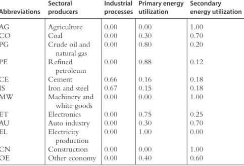
(4.9) The aggregate CO₂ emissions were captured in each sector (and region) from three origins: primary energy combustion (EE), secondary energy com-bustion (SE), and industrial processes (IND). In this specification, SE was due to the utilization of refined petroleum (RP), and emissions from IND were derived exclusively from iron and steel (IS), chemicals (CH), and cement (CE). The aggregate energy material balance data were used to map each sec-tor’s CO₂ emissions to these major sources using the summary in Table 4.1.

Distinct mechanisms were specified depending on the source of origin of the gaseous CO₂ eq. emissions. Emissions from EE activities were captured using Eq. (4.10), and emissions from SE of RP were captured using Eq. (4.11).

a Q CO j i R j i R j i R Sj i R 2EE, , =ε , , , , , , (4.10) z a Q CO i R i R i R S i R 2SERP, , = RP, , RP, , RP, , (4.11) Ei,R=Ai,RECO,i,RINCO,i,R −ρi,R+PG,i,RINPG,i,R−ρi, R+EL,i,RINEL,i,R−ρi,R−1 /ρi,R INCO,i,RINEL,i,R=CO,i,R1 −CO,i,R−PG,i,RPEL,i,R1+ tCO,i,RENVPCO,i,Rσi,R INPG,i,RINEL,i,R=PG,i,R1 −CO,i,R−PG,i,RPEL,i,R1+ tPG,i,RENVPPG,i,Rσi,R λK,i,R+λLA,i,R=1 CO₂EEj,i,R=εj,i,Raj,i,RQj,i,RS CO₂SERP,i,R=zRP,i,RaRP,i,R QRP,i,RS

The parameter ε_j,i,R in Eq. (4.10) summarizes the energy use coefficients (calibrated from the material energy balances tables) to set the composi-tion of emissions from primary energy via the combuscomposi-tion of CO and PG in each sector. The z_RP,i,R parameter in Eq. (4.11) similarly represents the emission coefficient due to the combustion of RP. The traditional I/O coefficient, a Q IN j i j i iS , ,

= , is responsive to price signals via optimizating costs, given technology (4.3). This is in contrast to traditional CGE analyses where a_j,i is typically regarded as fixed, as in a Leontieff technology.

Emissions from IND were recognized from IS, CH, and CE. These emissions were regarded as proportional to their respective real output (as shown in Eq. (4.12): Q i CO_{i R}IND IS,CH,CE i R i RS 2 , =η, , ∈

{

}

(4.12) Emissions from agricultural processes were similarly set proportionally to agricultural gross outputs. Emissions of non-CO₂ gasses (CH₄, F, and NO₂) were set proportionally to the EE activities. Thus CO₂ eq. emissions of CH₄ were calculated as shown in Eq. (4.13) and CH₄ from waste was calculated as per Eq. (4.14).

aj,i=INj,iQiS

CO₂INDi,R=ηi,RQi,RS i∈I S,CH,CE

Table 4.1 Distribution of CO₂ emissions from sectoral production activities by their source of origin Abbreviations Sectoral producers Industrial processes Primary energy utilization Secondary energy utilization AG Agriculture 0.00 0.00 1.00 CO Coal 0.00 0.30 0.70

PG Crude oil and

natural gas 0.00 0.80 0.20

PE Refined

petroleum 0.00 0.88 0.12

CE Cement 0.66 0.16 0.18

IS Iron and steel 0.67 0.15 0.18

MW Machinery and white goods 0.00 0.00 1.00 ET Electronics 0.00 0.75 0.25 AU Auto industry 0.00 0.30 0.70 EL Electricity production 0.00 1.00 0.00 CN Construction 0.00 0.00 1.00 OE Other economy 0.00 0.40 0.60

a Q j CO j i R for CO,PG j i R j i R i RS 2CH, ,4 =ε , , , , , =

{

}

(4.13) Q CO j i R j i R i RS 2WST, , =ϖ , , , (4.14) Household demand for energy generates an additional source of CO₂ eq. emissions. This was regarded as proportional to the household consump-tion of basic fuels (CO and RP) and calculated as in Eq. (4.15):

K C CO _{i i}D i 2HH CO,RP

∑

= ∈ (4.15) Aggregate CO₂ eq. emissions were calcualted as the sum of each of these sources (as shown in Eq. (4.16)):

CO CO CO CO CO CO CO CO j i R j i R j i R j i R j i R i R R R i 2TOT 2 , ,EE 2 , ,SE 2 , ,CH 2 , ,WST , , 2 ,IND 2AGR 2HH IS,CE 4

∑

∑

∑

(

)

= + + + + + + + ∈ (4.16)

4.2.3 Labor Markets, Income Generation, and General

Equilibrium

The model distinguishes two types of labor: urban (formal) and informal. The formal wage rate is fixed and the formal labor market adjusts with unemployment in each period. The flexibility of the real wage in the infor-mal labor market is characterized by the extent of fragmentation across the dualistic labor market in the Turkish economy. Data from different sectors and labor types were compiled from various TurkStat data sources. TurkStat provides sectoral labor employment data at the Nace Rev. 2 four-digit level, and regional formal–informal employment disaggregation data for the ma-jor sectors (i.e., agriculture, industry, and services) at the NUTS-2 level. The comprehensive treatment of both datasets makes it possible to approximate the sectoral formal and informal employment figures for both regions. In addition, the household labor force surveys (HLFS) from TurkStat were also used to determine the sectoral formal and informal wage ratios for the Nace Rev. 2, level 1. Hence total employment and total payments were obtained for each labor category in each region to enable calibration of the necessary parameters of the labor market.

The formal labor market was hypothesized to clear by quantity adjust-ments on employment (as shown in Eq. (4.17)):

U _R LS _R LF i RD i LF, = LF, −

∑

, (4.17) CO₂CH₄j,i,R=εj,i,Raj,i,RQi,R S forj=CO,PG CO₂WSTj,i,R=ϖj,i,RQi,RS CO₂HH=∑i∈CO,RPkiCiD CO₂TOT=∑j,i,RCO₂EEj,i,R+ CO₂SEj,i,R+CO₂CH₄j,i,R+CO 2WSTj,i,R+∑i∈IS,CECO2IND i,R+∑RCO₂AGRR+CO₂HH ULF,R=LLF,RS−∑iLFi,RD

Conversely, the informal or vulnerable labor market operates with fully flexible wages. The low level of informal wages is a symptomatic proxy for poverty in the informal labor market.

The regional labor markets have been linked by migration over time. This is based on (expected) wage differences between high- and low-in-come Turkey, and is driven along the classic Harris and Todaro (1970) speci-fication. Given the migrants from each labor type (l):

t E W W W L MIG_{l l} l l l l S ,RH ,RL ,RL .RL µ

(

)

( )

=    −        (4.18) where E[W_l,RH] is the expected wage rate of labor type l (=LF, LI) in the high-income region and µ_l is a calibration parameter (as shown in Eq. (4.18)).

Given that MIG_l(t) is based on wage expectations from high-income regions, labor supplies evolve according to Eq. (4.19):

L t n L t t L t n L t t 1 1 MIG 1 1 MIG l S l Sl l l S l Sl l ,RL ,RL ,RL ,RH ,RH ,RH

(

)

(

)

(

)

( )

( )

(

)

( )

( )

+ = + − + = + + (4.19) Capital stocks evolve given the net of depreciation of fixed invest-ments. The allocation of aggregate net investment funds to specific sectors (investment by destination sector) is accomplished through the calculation of regional profitability. Given sectorial profit rates (r_i,R) across regions, and the economy-wide average profit rate (rAVG_{), sectorial investment allocations} (∆K_i,R(t + 1)) are given by the simple rule in Eq. (4.20):

K t r r 1 i R i R i R i R r i R , , , , , AVG

(

)

∆ + = ∏ + ∏         − (4.20) where Π_i,R is the share of aggregate profits in sector, i, and region, R. This sets the allocation of physical investments to be reused via profit differences in the second part of the equation.

Private household income is composed of wage incomes from labor and remittances of profits from the enterprise sector. Public sector revenues comprise tax revenues (i.e., from wage and capital incomes) and nontaxa-tion sources of income (i.e., from various exogenous flows). The income flow of the public sector is further augmented by indirect taxes and envi-MIGlt=µlEWl,RH−Wl,RLWl,RLLl,RLS

Ll,RLSt+1=1+nl,RLLl, RLSt−MIGltLl,RHSt+1-=1+nl,RHLl,RHSt+MIGlt

ronmental taxes. This model closely follows the fiscal budget constraints. Given public earnings, the government’s “transfer expenditures to house-holds” were adjusted endogenously to sustain other components of pub-lic demand (i.e., pubpub-lic investment and consumption expenditure) as fixed ratios to the national income.

General equilibrium of the system was obtained via endogenous solu-tions on prices, wage rates, and the exchange rate. Informal wage rates across regions clear regional labor markets. The balance of payments is cleared through flexible adjustments on the real exchange rate (the ratio of the price of domestic goods to imports in the CGE folklore), while the nominal conversion factor across domestic and world prices serves as the numeraire of the system.

The model was solved iteratively by updating the annual “solutions” of the model to 2030. Aggregate output supplies grew through three channels: (1) the exogenous growth of labor supplies; (2) investments on physical capital net of depreciation; and (3) TFP growth, which in turn was regarded as exogenous. Capital stocks across regions and sectors were augmented with net investments in each period. Regional labor supplies were increased exogenously by population growth and migration (see Eq. (4.18)). TFP rates were updated in a Hicks-neutral manner, and formal real wage rates were updated by the cost of living index (endogenously solved).

4.3 DATA SOURCES AND CALIBRATION METHODOLOGY

4.3.1 Construction of the Regional Social Accounting

Database

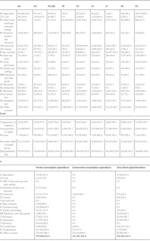
Regional I/O data are not available in Turkey, and the most recent I/O data was tabulated in 2012 by TurkStat. Given the lack of official regional data, regional economic activities were differentiated based on the standard tools of CGE applications. The SAM for 2012 (published by TurkStat) was generated using national income data on macroaggregates. Labor remu-nerations were obtained from the International Labor Organization (ILO) and TurkStat HLFS data. The aggregated I/O table for 2012 is displayed in Table 4.2.

Following production of the regional SAM (available upon request), the national macroaggregates were decomposed via the shares of gross regional value added. Based on the differentiation of level 2 NACE-1 data, 7 regions

Table 4.2 Turkey: I/O flow, 2012 (thousand TRY, at basic prices) (a) AG CO PG-OM PE CH CE IS PA FD TE MW ET AU EL CN TR OE Total intermediate exp AG: Agriculture 29,438,100.0 78,743.9 54,546.9 342.8 627,218.4 29,432.2 1,626.7 329,948.4 56,673,900.0 5,963,512.0 6,837.4 7,643.8 13.3 218.1 114,145.0 14,755.5 6,983,250.0 100,324,234.4 CO: Coal 241,156.8 1,812,815.0 46,806.7 0.0 51,800.0 1,212,684.0 9,904.6 5,596.6 11,085.5 39,119.1 10,533.4 2,043.2 17,471.2 2,892,929.0 150,131.4 369,767.5 3,420,575.0 10,294,419.0 PG-OM: Crude petrol, gas, and other mining 210,906.6 7,552.8 79,146.8 31,949,853.4 2,421,500.3 6,996,719.6 9,773,476.0 262,898.8 828,376.9 1,049,632.2 189,652.8 131,751.2 132,587.2 25,263,600.0 4,752,312.0 48,579.8 342,494.6 84,441,041.0 PE: Petroleum products and chemicals 4,463,786.0 482,505.4 1,413,983.2 896,789.5 881,275.0 1,805,806.0 404,557.2 103,165.7 655,855.6 393,888.5 392,764.6 434,782.5 104,590.8 402,526.5 4,985,364.0 27,820,300.0 15,290,800.0 60,932,740.5 CH: Chemicals 8,943,774.0 149,786.5 518,011.9 34,323.7 39,930,000.0 2,138,284.0 2,203,785.0 3,010,425.0 5,654,674.0 11,970,200.0 2,063,803.0 3,963,530.0 2,521,522.0 74,998.0 9,011,344.0 2,505,050.0 19,249,500.0 113,943,011.0 CE: Cement 131,181.1 29,774.1 176,995.1 959.4 638,264.6 6,899,405.0 404,325.4 4,348.3 551,646.0 34,853.0 486,955.6 395,805.1 499,281.2 130,407.6 26,354,700.0 873,664.8 6,311,453.0 43,924,019.4 IS: Iron and steel 6,189.1 176,973.1 189,257.0 15,557.3 628,560.3 402,435.3 22,077,700.0 128,280.6 110,110.1 35,588.7 23,231,400.0 9,206,265.0 7,382,780.0 71,908.0 25,127,300.0 214,117.1 6,893,704.0 95,898,125.6 PA: Paper and

print

112,492.8 1,145.2 7,790.0 33,263.3 1,001,410.0 532,824.6 236,644.8 7,671,507.0 2,493,897.0 1,138,633.0 375,728.6 416,025.6 91,823.0 76,001.1 158,535.2 493,570.0 12,457,800.0 27,299,091.1 FD: Food

processing

6,367,557.0 1,287.7 35,888.5 8,423.0 163,603.6 35,275.8 15,534.0 120,936.4 23,837,200.0 532,843.7 53,060.9 22,277.6 9,271.1 20,740.3 112,564.6 192,790.3 22,277,700.0 53,806,954.4 TE: Textiles and

clothing 109,045.8 34,191.3 71,756.1 3,727.0 660,675.7 191,847.4 60,557.2 440,838.4 310,247.9 54,879,800.0 194,564.3 106,494.7 360,412.2 4,587.5 150,869.4 213,276.3 6,420,095.0 64,212,986.2 MW: Machinery and white goods 191,484.4 95,966.7 286,033.5 28,047.8 750,545.5 201,658.7 721,510.2 55,299.5 711,785.0 411,298.9 8,533,914.0 2,544,749.0 4,400,737.0 13,924.3 14,862,000.0 1,043,107.0 8,283,650.0 43,135,711.5 ET: Electronics 71,891.1 57,314.0 29,347.2 8,154.9 130,570.8 137,281.9 33,310.1 43,219.4 116,673.8 249,493.4 1,383,245.0 8,789,359.0 2,310,104.0 523,752.9 5,576,912.0 232,564.4 9,502,252.0 29,195,445.9 AU: Automotive 265,689.5 452.6 9,533.1 24.4 1,025.7 17,526.2 0.0 1,466.0 533.3 20.5 908,353.4 32,064.5 14,162,600.0 152.1 26,964.7 1,079,149.0 2,930,046.0 19,435,601.0 EL: Electricity 902,509.1 245,169.5 734,655.4 26,902.8 2,034,290.0 2,554,476.0 4,387,732.0 528,733.6 1,835,289.0 3,103,648.0 1,151,517.0 400,417.4 472,991.9 60,459,600.0 428,257.7 441,051.6 18,662,500.0 98,369,741.0 CN: Construc-tion 364,064.3 41,899.8 51,341.5 2,076.5 226,323.2 85,032.7 254,640.8 44,775.1 350,386.1 191,751.7 262,073.7 61,717.8 42,641.2 409,542.4 47,242,300.0 423,232.1 16,689,700.0 66,743,498.9 TR: Transporta-tion 2,578,411.0 245,772.3 1,498,623.4 862,801.1 3,252,146.0 1,882,996.0 4,523,179.0 1,073,265.0 7,004,565.0 3,072,462.0 3,406,436.0 1,669,822.0 1,988,092.0 519,813.8 5,737,816.0 40,418,700.0 33,450,400.0 113,185,300.6 OE: Other economy 7,502,169.0 619,327.6 3,218,933.1 1,689,206.0 11,925,900.0 6,085,395.0 31,673,200.0 4,342,108.0 20,183,500.0 16,494,100.0 9,727,960.0 7,780,041.0 7,605,626.0 4,763,437.0 35,747,500.0 38,953,100.0 257,395,000.0 465,706,502.7 Totals 1,490,848,424.1 Compensation of employees 3,194,349.0 2,931,077.0 2,350,736.8 490,184.0 9,417,064.0 6,014,431.0 4,865,445.0 2,898,136.0 13,409,100.0 19,660,200.0 11,817,200.0 5,591,437.0 5,157,910.0 3,486,053.0 28,437,900.0 17,995,900.0 300,861,000.0 438,578,122.8 Gross payments to capital 114,385,806.7 7,537,819.5 6,476,128.0 4,300,537.1 26,692,027.6 13,138,833.8 17,346,494.5 6,496,242.2 44,601,389.6 40,845,650.7 25,534,769.8 11,112,743.6 11,235,858.0 18,247,251.3 96,009,108.4 106,232,907.8 495,482,442.8 1,045,676,011.6 Net taxes −409,801.0 392,980.3 1,013,682.7 5,347,046.8 4,198,528.4 1,941,986.2 4,545,101.4 993,550.4 1,464,525.4 2,564,477.7 2,551,131.5 2,102,840.6 2,389,320.9 5,542,117.9 7,227,473.0 16,871,035.3 26,681,983.0 85,417,980.6 Total value added

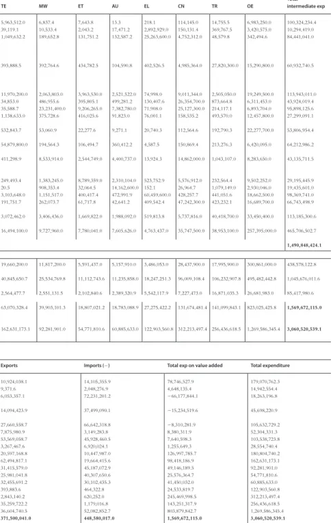
(at market prices) 117,170,354.7 10,861,876.9 9,840,547.5 10,137,767.9 40,307,620.0 21,095,251.0 26,757,040.9 10,387,928.7 59,475,015.0 63,070,328.4 39,903,101.3 18,807,021.2 18,783,088.9 27,275,422.2 131,674,481.4 141,099,843.1 823,025,425.8 1,569,672,115.0 Total production Exp 179,070,762.3 14,942,554.4 18,263,196.8 45,698,220.9 105,632,729.2 52,304,331.3 103,538,723.8 28,554,740.4 180,804,740.2 162,631,173.1 92,281,901.0 54,771,810.6 60,885,633.0 122,903,560.8 312,213,497.4 256,436,618.5 1,269,586,345.4 3,060,520,539.1 (b)

Private consumption expenditure Government consumption expenditure Gross fixed capital formation Exports Imports (−) Total exp on value added Total expenditure

AG: Agriculture 70,943,213.9 0.0 10,984,631.9 10,924,038.1 14,105,355.9 78,746,527.9 179,070,762.3

CO: Coal 6,163,732.6 0.0 523,308.1 9,371.6 2,048,276.9 4,648,135.4 14,942,554.4

PG-OM: Crude petrol, gas, and other mining

0.0 0.0 0.0 6,053,357.1 72,231,201.2 −66,177,844.1 18,263,196.8

PE: Petroleum products and chemicals

8,170,146.6 0.0 0.0 14,094,423.9 37,499,090.1 −15,234,519.6 45,698,220.9

CH: Chemicals 15,741,170.2 14,653,682.7 276,625.2 27,660,558.7 66,642,318.8 −8,310,281.9 105,632,729.2 CE: Cement 2,852,345.6 0.0 801,269.3 7,875,980.9 3,149,283.8 8,380,311.9 52,304,331.3

IS: Iron and steel 0.0 0.0 0.0 53,569,058.7 45,928,460.5 7,640,598.3 103,538,723.8

PA: Paper and print 4,908,205.9 0.0 0.0 3,267,467.6 6,920,024.1 1,255,649.3 28,554,740.4 FD: Food processing 116,848,603.9 0.0 0.0 20,597,168.8 10,447,987.0 126,997,785.7 180,804,740.2 TE: Textiles and clothing 55,215,191.4 0.0 372,594.0 62,494,817.1 19,664,415.6 98,418,186.9 162,631,173.1 MW: Machinery and white goods 3,885,275.6 0.0 59,032,407.9 31,415,579.0 45,187,072.9 49,146,189.5 92,281,901.0 ET: Electronics 17,821,133.8 0.0 22,081,839.7 25,981,041.8 40,307,650.6 25,576,364.7 54,771,810.6 AU: Automotive 17,253,690.8 0.0 21,843,085.3 32,455,691.2 30,102,435.3 41,450,032.0 60,885,633.0

EL: Electricity 24,604,258.9 0.0 0.0 393,883.6 464,322.8 24,533,819.7 122,903,560.8

CN: Construction 2,059,032.5 8,665.4 241,179,412.4 2,843,140.2 620,252.0 245,469,998.5 312,213,497.4 TR: Transportation 101,554,459.4 913,471.0 6,702,682.1 35,259,722.2 1,179,016.8 143,251,317.9 256,436,618.5 OE: Other economy 531,047,583.0 207,825,882.9 80,484,489.1 36,604,740.5 52,082,852.7 803,879,842.7 1,269,586,345.4

Table 4.2 Turkey: I/O flow, 2012 (thousand TRY, at basic prices) (a) AG CO PG-OM PE CH CE IS PA FD TE MW ET AU EL CN TR OE Total intermediate exp AG: Agriculture 29,438,100.0 78,743.9 54,546.9 342.8 627,218.4 29,432.2 1,626.7 329,948.4 56,673,900.0 5,963,512.0 6,837.4 7,643.8 13.3 218.1 114,145.0 14,755.5 6,983,250.0 100,324,234.4 CO: Coal 241,156.8 1,812,815.0 46,806.7 0.0 51,800.0 1,212,684.0 9,904.6 5,596.6 11,085.5 39,119.1 10,533.4 2,043.2 17,471.2 2,892,929.0 150,131.4 369,767.5 3,420,575.0 10,294,419.0 PG-OM: Crude petrol, gas, and other mining 210,906.6 7,552.8 79,146.8 31,949,853.4 2,421,500.3 6,996,719.6 9,773,476.0 262,898.8 828,376.9 1,049,632.2 189,652.8 131,751.2 132,587.2 25,263,600.0 4,752,312.0 48,579.8 342,494.6 84,441,041.0 PE: Petroleum products and chemicals 4,463,786.0 482,505.4 1,413,983.2 896,789.5 881,275.0 1,805,806.0 404,557.2 103,165.7 655,855.6 393,888.5 392,764.6 434,782.5 104,590.8 402,526.5 4,985,364.0 27,820,300.0 15,290,800.0 60,932,740.5 CH: Chemicals 8,943,774.0 149,786.5 518,011.9 34,323.7 39,930,000.0 2,138,284.0 2,203,785.0 3,010,425.0 5,654,674.0 11,970,200.0 2,063,803.0 3,963,530.0 2,521,522.0 74,998.0 9,011,344.0 2,505,050.0 19,249,500.0 113,943,011.0 CE: Cement 131,181.1 29,774.1 176,995.1 959.4 638,264.6 6,899,405.0 404,325.4 4,348.3 551,646.0 34,853.0 486,955.6 395,805.1 499,281.2 130,407.6 26,354,700.0 873,664.8 6,311,453.0 43,924,019.4 IS: Iron and steel 6,189.1 176,973.1 189,257.0 15,557.3 628,560.3 402,435.3 22,077,700.0 128,280.6 110,110.1 35,588.7 23,231,400.0 9,206,265.0 7,382,780.0 71,908.0 25,127,300.0 214,117.1 6,893,704.0 95,898,125.6 PA: Paper and

print

112,492.8 1,145.2 7,790.0 33,263.3 1,001,410.0 532,824.6 236,644.8 7,671,507.0 2,493,897.0 1,138,633.0 375,728.6 416,025.6 91,823.0 76,001.1 158,535.2 493,570.0 12,457,800.0 27,299,091.1 FD: Food

processing

6,367,557.0 1,287.7 35,888.5 8,423.0 163,603.6 35,275.8 15,534.0 120,936.4 23,837,200.0 532,843.7 53,060.9 22,277.6 9,271.1 20,740.3 112,564.6 192,790.3 22,277,700.0 53,806,954.4 TE: Textiles and

clothing 109,045.8 34,191.3 71,756.1 3,727.0 660,675.7 191,847.4 60,557.2 440,838.4 310,247.9 54,879,800.0 194,564.3 106,494.7 360,412.2 4,587.5 150,869.4 213,276.3 6,420,095.0 64,212,986.2 MW: Machinery and white goods 191,484.4 95,966.7 286,033.5 28,047.8 750,545.5 201,658.7 721,510.2 55,299.5 711,785.0 411,298.9 8,533,914.0 2,544,749.0 4,400,737.0 13,924.3 14,862,000.0 1,043,107.0 8,283,650.0 43,135,711.5 ET: Electronics 71,891.1 57,314.0 29,347.2 8,154.9 130,570.8 137,281.9 33,310.1 43,219.4 116,673.8 249,493.4 1,383,245.0 8,789,359.0 2,310,104.0 523,752.9 5,576,912.0 232,564.4 9,502,252.0 29,195,445.9 AU: Automotive 265,689.5 452.6 9,533.1 24.4 1,025.7 17,526.2 0.0 1,466.0 533.3 20.5 908,353.4 32,064.5 14,162,600.0 152.1 26,964.7 1,079,149.0 2,930,046.0 19,435,601.0 EL: Electricity 902,509.1 245,169.5 734,655.4 26,902.8 2,034,290.0 2,554,476.0 4,387,732.0 528,733.6 1,835,289.0 3,103,648.0 1,151,517.0 400,417.4 472,991.9 60,459,600.0 428,257.7 441,051.6 18,662,500.0 98,369,741.0 CN: Construc-tion 364,064.3 41,899.8 51,341.5 2,076.5 226,323.2 85,032.7 254,640.8 44,775.1 350,386.1 191,751.7 262,073.7 61,717.8 42,641.2 409,542.4 47,242,300.0 423,232.1 16,689,700.0 66,743,498.9 TR: Transporta-tion 2,578,411.0 245,772.3 1,498,623.4 862,801.1 3,252,146.0 1,882,996.0 4,523,179.0 1,073,265.0 7,004,565.0 3,072,462.0 3,406,436.0 1,669,822.0 1,988,092.0 519,813.8 5,737,816.0 40,418,700.0 33,450,400.0 113,185,300.6 OE: Other economy 7,502,169.0 619,327.6 3,218,933.1 1,689,206.0 11,925,900.0 6,085,395.0 31,673,200.0 4,342,108.0 20,183,500.0 16,494,100.0 9,727,960.0 7,780,041.0 7,605,626.0 4,763,437.0 35,747,500.0 38,953,100.0 257,395,000.0 465,706,502.7 Totals 1,490,848,424.1 Compensation of employees 3,194,349.0 2,931,077.0 2,350,736.8 490,184.0 9,417,064.0 6,014,431.0 4,865,445.0 2,898,136.0 13,409,100.0 19,660,200.0 11,817,200.0 5,591,437.0 5,157,910.0 3,486,053.0 28,437,900.0 17,995,900.0 300,861,000.0 438,578,122.8 Gross payments to capital 114,385,806.7 7,537,819.5 6,476,128.0 4,300,537.1 26,692,027.6 13,138,833.8 17,346,494.5 6,496,242.2 44,601,389.6 40,845,650.7 25,534,769.8 11,112,743.6 11,235,858.0 18,247,251.3 96,009,108.4 106,232,907.8 495,482,442.8 1,045,676,011.6 Net taxes −409,801.0 392,980.3 1,013,682.7 5,347,046.8 4,198,528.4 1,941,986.2 4,545,101.4 993,550.4 1,464,525.4 2,564,477.7 2,551,131.5 2,102,840.6 2,389,320.9 5,542,117.9 7,227,473.0 16,871,035.3 26,681,983.0 85,417,980.6 Total value added

(at market prices) 117,170,354.7 10,861,876.9 9,840,547.5 10,137,767.9 40,307,620.0 21,095,251.0 26,757,040.9 10,387,928.7 59,475,015.0 63,070,328.4 39,903,101.3 18,807,021.2 18,783,088.9 27,275,422.2 131,674,481.4 141,099,843.1 823,025,425.8 1,569,672,115.0 Total production Exp 179,070,762.3 14,942,554.4 18,263,196.8 45,698,220.9 105,632,729.2 52,304,331.3 103,538,723.8 28,554,740.4 180,804,740.2 162,631,173.1 92,281,901.0 54,771,810.6 60,885,633.0 122,903,560.8 312,213,497.4 256,436,618.5 1,269,586,345.4 3,060,520,539.1 (b)

Private consumption expenditure Government consumption expenditure Gross fixed capital formation Exports Imports (−) Total exp on value added Total expenditure

AG: Agriculture 70,943,213.9 0.0 10,984,631.9 10,924,038.1 14,105,355.9 78,746,527.9 179,070,762.3

CO: Coal 6,163,732.6 0.0 523,308.1 9,371.6 2,048,276.9 4,648,135.4 14,942,554.4

PG-OM: Crude petrol, gas, and other mining

0.0 0.0 0.0 6,053,357.1 72,231,201.2 −66,177,844.1 18,263,196.8

PE: Petroleum products and chemicals

8,170,146.6 0.0 0.0 14,094,423.9 37,499,090.1 −15,234,519.6 45,698,220.9

CH: Chemicals 15,741,170.2 14,653,682.7 276,625.2 27,660,558.7 66,642,318.8 −8,310,281.9 105,632,729.2 CE: Cement 2,852,345.6 0.0 801,269.3 7,875,980.9 3,149,283.8 8,380,311.9 52,304,331.3

IS: Iron and steel 0.0 0.0 0.0 53,569,058.7 45,928,460.5 7,640,598.3 103,538,723.8

PA: Paper and print 4,908,205.9 0.0 0.0 3,267,467.6 6,920,024.1 1,255,649.3 28,554,740.4 FD: Food processing 116,848,603.9 0.0 0.0 20,597,168.8 10,447,987.0 126,997,785.7 180,804,740.2 TE: Textiles and clothing 55,215,191.4 0.0 372,594.0 62,494,817.1 19,664,415.6 98,418,186.9 162,631,173.1 MW: Machinery and white goods 3,885,275.6 0.0 59,032,407.9 31,415,579.0 45,187,072.9 49,146,189.5 92,281,901.0 ET: Electronics 17,821,133.8 0.0 22,081,839.7 25,981,041.8 40,307,650.6 25,576,364.7 54,771,810.6 AU: Automotive 17,253,690.8 0.0 21,843,085.3 32,455,691.2 30,102,435.3 41,450,032.0 60,885,633.0 EL: Electricity 24,604,258.9 0.0 0.0 393,883.6 464,322.8 24,533,819.7 122,903,560.8 CN: Construction 2,059,032.5 8,665.4 241,179,412.4 2,843,140.2 620,252.0 245,469,998.5 312,213,497.4 TR: Transportation 101,554,459.4 913,471.0 6,702,682.1 35,259,722.2 1,179,016.8 143,251,317.9 256,436,618.5 OE: Other economy 531,047,583.0 207,825,882.9 80,484,489.1 36,604,740.5 52,082,852.7 803,879,842.7 1,269,586,345.4

were distinguished as “high income” and 19 regions were classified as “low income.” Data revealed that the low-income regions host approximately 60% of the total 73.7 million population, and produce around 32% of the aggregate value added. The remaining 68% of the aggregate value added originated in the high-income region. Further specifics of the regional mac-rodata are provided in Table 4.3.

The SAM tabulates the microlevel I/O data with the aggregate mac-rodata on public sector balances and resolves the saving–investment equi-librium. The latter discloses a current account deficit (foreign savings) of TRY 86,135.6 million (roughly 6.5% to the GDP). High- versus low-income Turkey yield the production activities, while components of aggregate na-tional demand were revealed using imperfect substitution in demand, and were calibrated through standard methods of the Armingtonian composite system.

This procedure was definitely a poor alternative to more direct ap-proaches based on regionally-differentiated production structures. However, this requires regional I/O data and regional material balances. In the absence of official or independent regional data, the Armingtonian imperfect substi-tutability framework based on cost optimization was utilized.

It is of note that the specification here was designed to only capture the regionally-differentiated component of (investment) subsidization. There-fore it should not be regarded as a detailed structural characterization of the dualistic (fragmented) patterns of production attributable to the Turkish economy, which is an issue beyond the scope of this paper.

Table 4.3 Economic indicators across regions (million TRY, 2012)

Region Gross re-gional value added Employ-ment of for-mal labor (thousand persons) Employ-ment of in-formal labor (thousand persons) Regional exports Taxes on production and em-ployment High-incomea 1,099,689.6 11,054.9 6,111.7 295,561.4 138,472.5 Low-incomeb 296,848.9 3,517.8 4,136.6 75,938.6 34,661.1

a _{High-income regions: TR10, TR21, TR31, TR41, TR42, TR51, and TR61.}

b _{Low-income regions: TR62, TR63, TR71, TR72, TR81, TR82, TR83, TR90, TR52, TR53, TR32,} TR33, TR22, TRA1, TRB1, TRB2, TRC1, TRC2, and TRC3.

4.3.2 Parametrization of Gaseous Pollutants

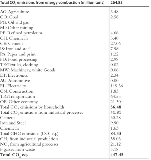
A total of 447.45 million tons of CO₂ eq. were reportedly released in Turkey in 2012. TurkStat data distinguished this sum into four sources (million tons): energy combustion (264.8), industrial processes (41.8), agricultural processes (21.2), and waste (56.5). Using a different level of aggregation, emissions of CO₂, CH₄, N₂O, and F-gasses accounted for 363.1, 58.0, 21.1, and 5.2 million tons of this total, respectively.

To direct these data into sectorial sources of origin, TurkStat data report-ed to the UNFCCC inventory system was usreport-ed. Where possible, original data on greenhouse gas source and sink categories were used to make direct connections between the sectors in the official dataset and the sectors dis-tinguished in this model (i.e., agriculture, refined petroleum, cement, iron and steel, and electricity). The remaining unaccounted CO₂ emissions were allocated to the aggregate using the share of the sectorial intermediate input demand. This exercise yielded CO₂ eq. emissions across production sectors and other activities as shown in Table 4.4.

Data in Table 4.4 was initially used to calculate the total sectorial emis-sions, CO_iTOT

2 . This sum was decomposed into three main sources of

ori-gin: emissions from EE, SE, and IND. This was performed using Table 4.1. Assuming π_s,i (s∈EE,SE,IND) is a typical element of Table 4.1, then:

CO_{2 ,S i}=π_{S i,}.CO_2iTOT

The coefficient z_RP,i was subsequently calibrated by:

z CO IN i i i RP, 2RP,SE RP, =

For distinguishing this aggregate into the regional activities, regional shares of sectorial output were used. The source of CO₂ eq. emissions ide-ally ought to be used for regions; however, ad hoc specifications were not made due to the absence of precise regional data measurements. A similar procedure was followed to determine the EE sources of CO₂ eq. emissions across sectors (for j∈CO and PG) and CO EE_{j i}

2 , was found from data displayed

in Table 4.4 using the ε_j,i for j∈CO and PG.

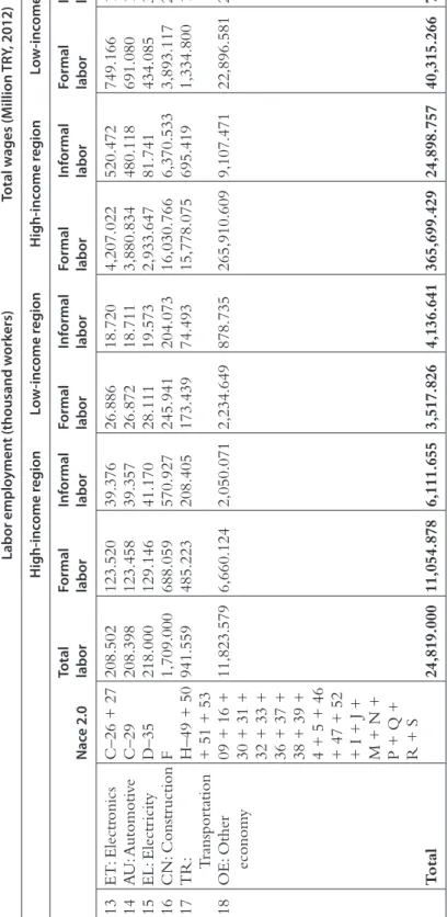
4.3.3 Calibration of the Labor Markets

Two types of labor were distinguished in the model: formal and informal. The characterization was based on the ILOs definition of informal

employ-CO₂TOTi

CO₂S,i=πS,i⋅CO₂TOTi

zRP,i=CO₂SERP,iINRP,i

ment, which is informal (unregistered employment that is under any social security coverage) + self-employed + unpaid family labor. Using this cri-teria, a total of 24,819 thousand workers was distributed across regions and sectors (using the HLFS TurkStat data). Table 4.5 shows parametrization of the labor markets.

The I/O wage and salary data is used to set the formal labor share in national income. Using this data, we used the formal and informal em-ployment shares from the HLFS data to produce aggregate wage income data for the informal labor. Finally, the sectorial and regional wage remu-nerations across labor types were obtained using the sectorial income shares from the I/O table. All data is summarized in Table 4.5.

Table 4.4 Aggregate CO₂ eq. emissions, 2012

Total CO₂ emissions from energy combustion (million tons) 264.83

AG: Agriculture 3.48

CO: Coal 2.58

PG: Oil and gas MI: Other mining

PE: Refined petroleum 4.66

CH: Chemicals 5.40

CE: Cement 27.06

IS: Iron and steel 7.98

PA: Paper and print 1.22

FD: Food processing 2.98

TE: Textiles, clothing 0.02

MW: Machinery, white Goods 0.06

ET: Electronics 2.34

AU: Automotive 0.00

EL: Electricity 119.36

CN: Construction 1.83

TR: Transportation 64.55

OE: Other economy 21.30

Total CO₂ emissions by households 56.48

Total CO₂ emissions from industrial processes 41.81

Cement 30.28

Iron and Steel 9.90

Chemicals 1.63

Total GHG emissions (CO₂ eq.) 84.33

CH₄ from industrial production 58.03

NO₂ from agricultural processes 21.12

F gasses from waste 5.18

Table 4.5

P

ar

amet

ers of the labor mar

ket, 2012 Labor emplo ymen t (thousand w ork ers) Total w ages (M illion TR Y, 2012) H igh-inc ome r eg ion Lo w -inc ome r eg ion H igh-inc ome r eg ion Lo w -inc ome r eg Nac e 2.0 Total labor Formal labor Inf ormal labor Formal labor Inf ormal labor Formal labor Inf ormal labor Formal labor Inf ormal labor 1 A G: Ag ricultur e A–01, 02, 03 6,097.000 692.000 2,493.000 307.211 2,606.789 1,195.328 1,090.099 208.377 700.545 2 CO: Coal B–05 51.024 34.925 4.939 9.778 1.383 2,328.745 93.190 493.105 16.037 3 PG+OM: P etr

o-leum gas and other mining

B–06 + 07 + 08 79.884 54.679 7.732 15.308 2.165 1,843.365 99.038 395.472 12.862 5 PE: Refined _petr oleum C–19 10.042 6.874 0.972 1.924 0.272 366.157 23.386 97.604 3.037 6 CH: Chemicals C–20 + 21 + 22 365.705 216.649 69.065 47.157 32.834 7,085.441 876.576 1,261.741 193.306 7 CE: Cement C–23 294.571 174.508 55.631 37.984 26.448 4,525.285 559.846 805.841 123.460 8 IS: Ir on and steel C–24 154.330 91.428 29.146 19.900 13.856 3,660.782 452.894 651.894 99.874 9 PA: P aper and pr int C–17 + 18 148.416 87.924 28.029 19.138 13.325 2,180.570 269.769 388.305 59.491 10 FD: F ood pr ocessing C–10 + 11 + 12 594.080 351.942 112.195 76.605 53.338 10,089.067 1,248.170 1,796.612 275.252 11 TE: T extiles and clothing C–13 + 14 + 15 1,267.238 750.731 239.324 163.407 113.777 14,792.422 1,830.046 2,634.163 403.569 12 MW : Machiner y

and white goods

C–25 + 28 647.672 383.690 122.316 83.516 58.150 8,891.314 1,099.990 1,583.322 242.574 _(Continued

Labor emplo ymen t (thousand w ork ers) Total w ages (M illion TR Y, 2012) H igh-inc ome r eg ion Lo w -inc ome r eg ion H igh-inc ome r eg ion Lo w -inc ome r Nac e 2.0 Total labor Formal labor Inf ormal labor Formal labor Inf ormal labor Formal labor Inf ormal labor Formal labor 13 ET : Electr onics C–26 + 27 208.502 123.520 39.376 26.886 18.720 4,207.022 520.472 749.166 14 A U: Automoti ve C–29 208.398 123.458 39.357 26.872 18.711 3,880.834 480.118 691.080 15 EL: Electr icity D–35 218.000 129.146 41.170 28.111 19.573 2,933.647 81.741 434.085 16 CN: Constr uction F 1,709.000 688.059 570.927 245.941 204.073 16,030.766 6,370.533 3,893.117 17 TR: T ranspor tation H–49 + 50 + 51 + 53 941.559 485.223 208.405 173.439 74.493 15,778.075 695.419 1,334.800 18 OE: Other _econom y 09 + 16 + 30 + 31 + 32 + 33 + 36 + 37 + 38 + 39 + 4 + 5 + 46 + 47 + 52 + I + J + M + N + P + Q + R + S 11,823.579 6,660.124 2,050.071 2,234.649 878.735 265,910.609 9,107.471 22,896.581 T otal 24,819.000 11,054.878 6,111.655 3,517.826 4,136.641 365,699.429 24,898.757 40,315.266 Source: Author s’ calculations fr om TurkStat, Household Labor F or ce Sur ve ys. Table 4.5 P ar amet

ers of the labor mar

ket, 2012 (

Cont.

REFERENCES

Acar, S., Yeldan, A.E., March 2016. Environmental impacts of coal subsidies in Turkey: a gen-eral equilibrium analysis. Energy Policy 90, 1–15.

Agénor, P.R., 2004. Macroeconomic adjustment and the poor: analytical issues and cross-country evidence. J. Econ. Surv. 18 (3), 351–408.

Agénor, P.-R., Izquierdo, A., Fofack, H., 2003. IMMPA: A Quantitative Macroeconomic Framework for the Analysis of Poverty Reduction Strategies. World Bank Policy Re-search Working Paper 3092. World Bank, Washington, DC.

Akın-Ölçüm, G., Yeldan, E., 2013. Economic impact assessment of Turkey’s post-Kyoto vi-sion on emisvi-sion trading. Energy Policy 60, 764–774.

Alzua, M.L., Ruffo, H., 2011. Effects of Argentina’s Social Security Reform on Labor Mar-kets and Poverty. MPIA Working Paper 2011-11.

Armington, P., 1969. A theory of demand for products distinguished by place of production. IMF Staff Pap. 16 (1), 159–178.

Bergman, L., 1990. The development of computable general equilibrium modeling. In: Bergman, L.J., Jorgenson, D.W., Zalai, E. (Eds.), General Equilibrium Modelling and Economic Policy Analysis. Basil Blackwell Press, pp. 3–30.

Bhattacharyya, S.C., 1996. Applied general equilibrium models for energy studies: a survey. Energy Econ. 18, 145–164.

Boeters, S., Savard, L., 2012. The labor market in computable general equilibrium models. Dixon, P., Jorgenson, D. (Eds.), Handbook of CGE Modeling, vol. 1b, North Holland.

Böhringer, C., 1998. The synthesis of bottom-up and top-down in energy modeling. Energy Econ. 20, 234–248.

Böhringer, C., Löschel, A., 2006. Computable general equilibrium models of sustainability impact assessment: status qua and prospects. Ecol. Econ. 60, 49–64.

de Melo, J.A.P., 1977. Distortions in the factor market: some general equilibrium estimates. Rev. Econ. Stat. 59 (4), 398–405.

Donaghy, K.P., 2009. CGE modeling in space: a survey. In: Capello, R., Nijkamp, P. (Eds.), Handbook of Regional Growth and Development Theories. Edward Elgar, Cheltenham.

Giesecke, J.A., Madden, J.R., 2012. Regional computable general equilibrium modeling. Dixon, P., Jorgenson, D. (Eds.), Handbook of CGE Modeling, vol. 1a, North Holland.

Gilbert, J., Wahl, T., 2002. Applied general equilibrium assessments of trade liberalization in China. World Econ. 25, 697–731.

Graafland, J.J., de Mooij, R.A., Nibbelink, A.G.H., Nieuwenhuis, A., 2001. MIMICing Tax Policies and the Labor Market. Elsevier, Amsterdam.

Harris, J.R., Todaro, M.P., 1970. Migration, unemployment and development: a two-sector analysis. Am. Econ. Rev. 60 (1), 126–142.

Hendy, R., Zaki, C., 2013. Assessing the effects of trade liberalization on wage inequalities in Egypt: a microsimulation analysis. Int. Trade J. 27 (1), 63–104.

Higgins, B., 1956. The ‘Dualistic Theory’ of Underdeveloped Areas. Economic Develop-ment and Cultural Change 4 (2), 99-115.

Jorgenson, D.W., 1961. The development of a dual economy. Econ. J. 71 (282), 309–334.

Jorgenson, D.W., 1966. Testing alternative theories of the development of a dual economy. In: Adelman, I., Thorbecke, E. (Eds.), The Theory and Design of Economic Development. Johns Hopkins, Baltimore.

Jorgenson, D.W., 1967. Surplus Agricultural Labor and the Development of a Dual Economy. Oxford Economic Papers, Oxford, pp. 288–312.

Khan, H.A., 2004. Using Macroeconomic Computable General Equilibrium Models for Assessing Poverty Impact of Structural Adjustment Policies, Asian Development Bank Institute Discussion Paper No. 12.

Kraybill, D.S., 1993. Computable general equilibrium analysis at the regional level. In: Otto, D.M., Johnson, T.G. (Eds.), Microcomputer-based Input-Output Modeling: Applications to Economic Development. Westview Press, Boulder.

Kumbarog˘lu, G.S., 2003. Environmental taxation and economic effects: a computable gen-eral equilibrium analysis for Turkey. J. Policy Model. 25, 795–810.

Lewis, W.A., 1954. Economic Development with Unlimited Supplies of Labour. Manchester School 22 (2), 139–191.

Lise, W., 2006. Decomposition of CO₂ emissions over 1980–2003 in Turkey. Energy Policy 34, 1841–1852.

Manne, A.S., 1981. ETA-MACRO: A User’s Guide. Electric Power Research Institute, Palo Alto, CA.

Morrone, H., 2016. Brazilian’s structural change and economic performance: structuralist comments on macroeconomic policies. Econ. Aplic. 20 (4), 473–488.

Partridge, M.D., Rickman, D.S., 2010. Computable general equilibrium (CGE) modeling for regional economic development analysis. Reg. Stud. 44, 1311–1328.

Pyatt, G., Round, J., 1979. Accounting and fixed price multipliers in a social accounting matrix framework. Econ. J. 89, 850–873.

Rada, C., von Armin, R., 2014. India’s structural transformation and role in the world econ-omy. J. Policy Model. 36 (1), 1–23.

Ranis, G., Fei, J.D.H., 1961. A theory of economic development. Am. Econ. Rev. 51, 533–565. Roson, R., van der Mensbrugghe, J., 2017. Demand-Driven Structural Change in Applied General Equilibrium Models. IEFE Working Papers 96, IEFE, Center for Research on Energy and Environmental Economics and Policy, Universita’ Bocconi, Milano, Italy. Şahin, Ş., 2004. An Economic Policy Discussion of the GHG Emission Problem in Turkey From

a Sustainable Development Perspective Within a Regional General equilibrium Model: TURCO (unpublished Ph.D. thesis). Université Paris I Panthéon, Sorbonne, submitted.

Shoven, J.B., Whalley, J., 1992. Applying General Equilibrium. Cambridge University Press, London.

Stifel, D.C., Thorbecke, E., 2003. A dual-dual CGE model of an archetype African economy: trade reform, migration and poverty. J. Policy Model. 25 (3), 207–235.

Sue Wing, I., 2004. CGE Models for Economy-Wide Policy Analysis. MIT Joint Program on the Science and Policy of Global Change, Technical Note No. 6.

Telli, Ç., Voyvoda, E., Yeldan, E., 2008. Economics of environmental policy in Turkey: a gen-eral equilibrium investigation of the economic evaluation of sectoral emission reduction policies for climate change. J. Policy Model. 30 (1), 321–340.

Temple, J.R.W., 2004. Dualism and Aggregate Productivity. CEPR Discussion Paper 4387.

Temple, J.R.W., 2005. Dual economy models: a primer for growth economists. Manch. Sch. 73 (4), 435–478.

Thorbecke, E., 1993. Impact of state and civil institutions on the operation of rural market and nonmarket configurations. World Dev. 21 (4), 591–605.

UNFCCC, 2013. GHG Inventories (Annex I), National Inventory Submissions 2013. Na-tional Report for Turkey. Available from: http://unfccc.int/national_reports/annex_i_ ghg_inventories/national_inventories_submissions/itms/8108.php.

Vural, B., 2009. General Equilibrium Modeling of Turkish Environmental Policy and the Kyoto Protocol (unpublished MA thesis). Bilkent University, submitted.

Yang, Y., Huang, Y., 1997. The Impact of Trade Liberalization on Income Distribution in China. Economics Division China Economy Working Paper 97/1.

Yeldan, A.E., Tas¸çı, K., Voyvoda, E., Özsan, M.E., March 2013. Escape from the Middle In-come Trap: Which Turkey? TURKONFED, Istanbul.

Yeldan, A.E., Tas¸çı, K., Özsan, M.E., Voyvoda, E., 2014. Planning for regional development: a general equilibrium analysis for Turkey. In: Yülek, M. (Ed.), Advances in General Equi-librium Modeling. Springer, pp. 291–331.

FURTHER READING

Voyvoda, E., Yeldan, E.A., 2011. Investigation of the Rational Steps Towards National Programme for Climate Change Mitigation (in Turkish). TR Ministry of Development, Ankara, mimeo.